$B^{0}\to\phi\phi$ Decay in Perturbative QCD Approach

Abstract

The rare decay $B^{0}\to\phi\phi$ can occur only via penguin annihilation topology in the standard model. We calculate this channel in the perturbative QCD approach. The predicted branching ratio is very small at ($10^{-8}$). We also give the polarization fractions, which shows that the transverse polarization contribution is comparable to the longitudinal one, due to a big transverse contribution from factorizable diagrams. The small branching ratio in SM, makes it sensitive to any new physics contributions.

1 Introduction

The study of B meson decays has offered a good place to test the standard model (SM) and to give some important constraints on the SM parameters. Recently, more attentions have been paid to the $B\rightarrow VV$ decay modes. The transverse polarization of the vector meson can contribute to the decay width, and the fraction of each kind of polarization has been or will be measured. In some penguin dominated decay modes, such as $B\rightarrow\phi K^{\ast}$ [1], the experimental results for polarization differ from most theoretical predictions [2], which has been considered as a puzzle and lots of discussions have been given [3, 4]. So the polarization problem in the $B\rightarrow VV$ decay modes brings a new challenge to the standard model, maybe it is a signal of new physics [4, 5].

In this work we will calculate the branching ratio and the polarization fractions of the charmless decay channel $B^{0}\rightarrow\phi\phi$ with perturbative QCD approach (PQCD) [6, 7]. In this channel, the initial $\bar{b}$ quark and the light valence $d$ quark in the $B$ meson don’t appear in the final states, so it must be an annihilation topology in Feynman diagrams. Annihilation diagrams can’t be calculated in factorization approach [8, 9] or in QCD improved factorization approach [10] for its endpoint singularity, but in PQCD approach this singularity can be regulated by Sudakov form factor and threshold resummation, so the PQCD calculations can give converging results and have prediction power. In this channel, since no tree level operators can contribute, the dominant contribution comes from penguin operators. The annihilation topology is usually suppressed relative to the emission topology which can appear in other modes, so this channel is a rare decay mode, and hasn’t been measured in the $B$ factories.

In the next section we give our theoretical formulae based on the PQCD framework. Then we show the numerical results and a brief conclusion in the third section.

2 Perturbative calculation

For simplicity, we work in the B meson rest frame, and adopt the light-cone coordinate system. Then the four-momentum of the B meson and the two $\phi$ mesons in the final state can be written as:

$$P_{1}=\frac{M_{B}}{\sqrt{2}}(1,1,{\bf 0_{T}}),$$

$$P_{2}=\frac{M_{B}}{\sqrt{2}}(1-r,r,{\bf 0_{T}}),$$

$$P_{3}=\frac{M_{B}}{\sqrt{2}}(r,1-r,{\bf 0_{T}}),$$ (1)

in which $r$ is defined by $r=\frac{1}{2}(1-\sqrt{1-4M_{\phi}^{2}/M_{B}^{2}})\simeq M_{\phi}^{2}/M_{B}^{2}\ll 1$. To extract the helicity amplitudes, we should parameterize the polarization vectors. The longitudinal polarization vector must satisfy the orthogonality and normalization: ${\epsilon_{2L}\cdot P_{2}}=0,\,\,{\epsilon_{3L}\cdot P_{3}}=0$, and ${\epsilon_{2L}}^{2}={\epsilon_{3L}}^{2}=-1$. Then we can give the manifest form as follows:

$${\epsilon_{2L}}=\frac{1}{\sqrt{2r}}(1-r,-r,{\bf 0_{T}}),$$

$${\epsilon_{3L}}=\frac{1}{\sqrt{2r}}(-r,1-r,{\bf 0_{T}}).$$ (2)

As to the transverse polarization vectors, we can choose the simple form:

$${\epsilon_{2T}}=\frac{1}{\sqrt{2}}(0,0,{\bf 1_{T}}),$$

$${\epsilon_{3T}}=\frac{1}{\sqrt{2}}(0,0,{\bf 1_{T}}).$$ (3)

Only penguin operators can contribute to this decay channel, so the relevant effective weak Hamiltonian can be written as [11]:

$${\cal H}_{eff}=\frac{G_{F}}{\sqrt{2}}V_{tb}V_{td}^{*}C_{i}(\mu)O_{i}(\mu),\,\,\,\,i=3-10,$$ (4)

where $C_{i}$ are QCD corrected Wilson coefficients, and $O_{i}$ are the usual penguin operators with the form

$$\begin{array}[]{ll}O_{3}=(\bar{s}_{i}b_{i})_{V-A}\sum\limits_{q}(\bar{q}_{j}q_{j})_{V-A},&O_{4}=(\bar{s}_{i}b_{j})_{V-A}\sum\limits_{q}(\bar{q}_{j}q_{i})_{V-A}\\ O_{5}=(\bar{s}_{i}b_{i})_{V-A}\sum\limits_{q}(\bar{q}_{j}q_{j})_{V+A},&O_{6}=(\bar{s}_{i}b_{j})_{V-A}\sum\limits_{q}(\bar{q}_{j}q_{i})_{V-A},\\ O_{7}=\frac{3}{2}(\bar{s}_{i}b_{i})_{V-A}\sum\limits_{q}e_{q}(\bar{q}_{j}q_{j})_{V+A},&O_{8}=\frac{3}{2}(\bar{s}_{i}b_{j})_{V-A}\sum\limits_{q}e_{q}(\bar{q}_{j}q_{i})_{V+A},\\ O_{9}=\frac{3}{2}(\bar{s}_{i}b_{i})_{V-A}\sum\limits_{q}e_{q}(\bar{q}_{j}q_{j})_{V-A},&O_{10}=\frac{3}{2}(\bar{s}_{i}b_{j})_{V-A}\sum\limits_{q}e_{q}(\bar{q}_{j}q_{i})_{V-A}.\end{array}$$ (5)

where $q=s$. The first four operators are QCD penguin operators; while the last four are electroweak penguin operators, which should be suppressed by the coupling $\alpha/\alpha_{s}$.

The decay width for this channel is:

$$\Gamma=\frac{1}{2}\frac{G_{F}^{2}{\bf|P_{c}|}}{16\pi M_{B}^{2}}|V_{tb}^{*}V_{td}|^{2}\sum\limits_{\sigma=L,T}{\cal M}^{\sigma{\dagger}}{\cal M}^{\sigma},$$ (6)

where ${\bf P_{c}}$ is the 3-momentum of the final state meson, with $|{\bf P_{c}}|=\frac{M_{B}}{2}(1-2r)$. Note that for our case an additional factor $1/2$ should appear for the permutation symmetry of the identical final state particles. The decay amplitude ${\cal M}^{\sigma}$ which is decided by QCD dynamics will be calculated later in PQCD approach. The subscript $\sigma$ denotes the helicity states of the two vector mesons with L(T) standing for the longitudinal (transverse) components. After analyzing the Lorentz structure, the amplitude can be decomposed into [1]:

$${\cal M}^{\sigma}=M_{B}^{2}{\cal M}_{L}+M_{B}^{2}{\cal M}_{N}\epsilon^{\ast}_{2}(\sigma=T)\cdot\epsilon^{\ast}_{3}(\sigma=T)+i{\cal M}_{T}\epsilon_{\mu\nu\rho\sigma}\epsilon_{2}^{\mu\ast}\epsilon_{3}^{\nu\ast}P_{2}^{\rho}P_{3}^{\sigma}.$$ (7)

We can define the longitudinal $H_{0}$, transverse $H_{\pm}$ helicity amplitudes as

$$H_{0}=M^{2}_{B}{\cal M}_{L},\,\,H_{\pm}=M^{2}_{B}{\cal M}_{N}\mp M_{\phi}^{2}\sqrt{r^{\prime 2}-1}{\cal M}_{T},$$ (8)

where $r^{\prime}=(P_{2}\cdot P_{3})/{M_{\phi}^{2}}$. After the helicity summation, we can deduce that they satisfy the relation

$$\sum\limits_{\sigma=L,R}{\cal M}^{\sigma{\dagger}}{\cal M}^{\sigma}=|H_{0}|^{2}+|H_{+}|^{2}+|H_{-}|^{2}.$$ (9)

There is another equivalent set of definition of helicity amplitudes

$$A_{0}=-\xi M^{2}_{B}{\cal M}_{L},$$

$$A_{\|}=\xi\sqrt{2}M^{2}_{B}{\cal M}_{N},$$

$$A_{\perp}=\xi M_{\phi}^{2}\sqrt{r^{\prime 2}-1}{\cal M}_{T},$$ (10)

with $\xi$ the normalization factor to satisfy

$$|A_{0}|^{2}+|A_{\|}|^{2}+|A_{\perp}|^{2}=1,$$ (11)

where the notations $A_{0}$, $A_{\|}$, $A_{\perp}$ denote the longitudinal, parallel, and perpendicular polarization amplitude.

What is followed is to calculate the matrix elements ${\cal M}_{L}$, ${\cal M}_{N}$ and ${\cal M}_{T}$ of various operators in the weak Hamiltonian with PQCD approach. In PQCD approach, the decay amplitude is factorized into the convolution of the mesons’ light-cone wave functions, the hard scattering kernel and the Wilson coefficients, which stands for the soft, hard and harder dynamics respectively. The transverse momentum was introduced so that the endpoint singularity which will break the collinear factorization is regulated and the large double logarithm term appears after the integration on the transverse momentum, which is then resummed into the Sudakov form factor. The formalism can be written as:

$${\cal M}\sim \int dx_{1}dx_{2}dx_{3}b_{1}db_{1}b_{2}db_{2}b_{3}db_{3}Tr[C(t)\Phi_{B}(x_{1},b_{1})\Phi_{\phi}(x_{2},b_{2})\Phi_{\phi}(x_{3},b_{3})$$ (12)

$$H(x_{i},b_{i},t)S_{t}(x_{i})e^{-S(t)}],$$

where the $b_{i}$ is the conjugate space coordinate of the transverse momentum, which represents the transverse interval of the meson. $t$ is the largest energy scale in hard function $H$, while the jet function $S_{t}(x_{i})$ comes from the summation of the double logarithms $\ln^{2}x_{i}$, called threshold resummation [12], which becomes large near the endpoint.

The light cone wave functions of mesons are not calculable in principal in PQCD, but they are universal for all the decay channels. So that they can be constraint from the measured other decay channels, like $B\to K\pi$ and $B\to\pi\pi$ decays etc. [7]. For the heavy $B$ meson, we have

$$\frac{1}{\sqrt{2N_{c}}}(\not\!P_{1}+M_{B})\gamma_{5}\phi_{B}(x,b).$$ (13)

For the longitudinal polarized $\phi$ meson,

$$\frac{1}{\sqrt{2N_{c}}}[M_{\phi}\not\!\epsilon_{2L}\phi_{\phi}(x)+\not\!\epsilon_{2L}\not\!P_{2}\phi_{\phi}^{t}(x)+M_{\phi}I\phi^{s}_{\phi}(x)],$$ (14)

and for transverse polarized $\phi$ meson,

$$\frac{1}{\sqrt{2N_{c}}}[M_{\phi}\not\!\epsilon_{2T}\phi^{v}_{\phi}(x)+\not\!\epsilon_{2T}\not\!P_{2}\phi_{\phi}^{T}(x)+\frac{M_{\phi}}{P_{2}\cdot n_{-}}i\epsilon_{\mu\nu\rho\sigma}\gamma_{5}\gamma^{\mu}\epsilon_{2T}^{\nu}P_{2}^{\rho}n_{-}^{\sigma}\phi^{a}_{\phi}(x)].$$ (15)

In the following concepts, we omit the subscript of the $\phi$ meson for simplicity.

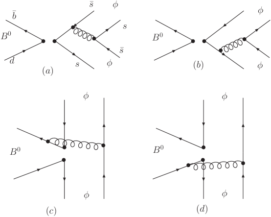
Figure 1: Leading order Feynman diagrams for $B^{0}\rightarrow\phi\phi$

Now the only thing left is the hard part $H$. In PQCD approach, it contains the corresponding four quark operator and the hard gluon connecting the quark pair from sea. They altogether make an effective six quark interaction. The hard part $H$ is channel dependent, but it is perturbative calculable. When calculating the hard parts (shown in the Figure 1), the factorizable diagrams (a) and (b) have strong cancellation effects, which results in null longitudinal polarization contribution and null parallel polarization contribution. The perpendicular polarization survives with a large factorizable contribution, which will be shown later to make a large transverse polarization. The detailed formulas with polarization ${\cal M}_{L}$, ${\cal M}_{N}$, and ${\cal M}_{T}$ for each diagram are given in the appendix. According to PQCD power counting rules, the longitudinal nonfactorizable diagram should give the leading contribution, and the contributions from the other diagrams are suppressed by a factor $r$.

3 Numerical results and summary

For the $B$ meson wave function distribution amplitude in eq.(13), we employ the model [7]

$$\phi_{B}(x)=N_{B}x^{2}(1-x)^{2}\exp\left[-\frac{1}{2}\left(\frac{xM_{B}}{\omega_{B}}\right)^{2}-\frac{\omega^{2}_{B}b^{2}}{2}\right],$$ (16)

where the shape parameter $\omega_{B}=0.4$GeV has been constrained in other decay modes. The normalization constant $N_{B}=91.784$GeV is related to the B decay constant $f_{B}=0.19$GeV. It is one of the two leading twist B meson wave functions; the other one is power suppressed, so we omit its contribution in the leading power analysis [13]. The $\phi$ meson distribution amplitude up to twist-3 are given by [14]

$$\phi_{\phi}(x)=\frac{3f_{\phi}}{\sqrt{2N_{c}}}x(1-x),$$ (17)

$$\phi^{t}_{\phi}(x)=\frac{f_{\phi}^{T}}{2\sqrt{2N_{c}}}\left\{3(1-2x)^{2}+1.68C_{4}^{\frac{1}{2}}(1-2x)+0.69\left[1+(1-2x)\ln{\frac{x}{1-x}}\right]\right\},$$ (18)

$$\phi^{s}_{\phi}(x)=\frac{f_{\phi}^{T}}{4\sqrt{2N_{c}}}\left[3(1-2x)(4.5-11.2x+11.2x^{2})+1.38\ln{\frac{x}{1-x}}\right],$$ (19)

$$\phi^{T}_{\phi}(x)=\frac{3f_{\phi}^{T}}{2\sqrt{2N_{c}}}x(1-x)\left[1+0.2C_{4}^{\frac{3}{2}}(1-2x)\right],$$ (20)

$$\phi^{v}_{\phi}(x)=\frac{f_{\phi}^{T}}{2\sqrt{2N_{c}}}\left\{\frac{3}{4}[1+(1-2x)^{2}]+0.24[3(1-2x)^{2}-1]+0.96C_{4}^{\frac{1}{2}}(1-2x)\right\},$$ (21)

$$\phi^{a}_{\phi}(x)=\frac{3f_{\phi}^{T}}{4\sqrt{2N_{c}}}(1-2x)[1+0.93(10x^{2}-10x+1)],$$ (22)

with the Gegenbauer polynomials,

$$C_{2}^{\frac{1}{2}}(\xi)=\frac{1}{2}(3\xi^{2}-1),$$ (23)

$$C_{4}^{\frac{1}{2}}(\xi)=\frac{1}{8}(35\xi^{4}-30\xi^{2}+3),$$ (24)

$$C_{2}^{\frac{3}{2}}(\xi)=\frac{3}{2}(5\xi^{2}-1).$$ (25)

We employ the constants as follows [15]: the Fermi coupling constant $G_{F}=1.16639\times 10^{-5}$GeV^-2, the CKM matrix element $|V_{tb}^{\ast}V_{td}|=0.0084$, the meson masses $M_{B}=5.28$GeV, $M_{\phi}=1.02$GeV, the decay constants $f_{\phi}=0.237$GeV, $f_{\phi}^{T}=0.22$GeV and the $B$ meson lifetime $\tau_{B^{0}}=1.55ps$. The results for the center value of the branching ratio is then

$$Br(B^{0}\rightarrow\phi\phi)=1.89\times 10^{-8},$$ (26)

and the helicity amplitudes are given by

$$R_{0}=0.65, R_{\|}=0.02, R_{\perp}=0.33,$$ (27)

which shows that the transverse polarization contribution is comparable to the longitudinal one. The relative strong phases, $\phi_{\|}=\arg{(A_{\|}/A_{0})}$, $\phi_{\perp}=\arg{(A_{\perp}/A_{0}})$ are given by

$$\phi_{\|}=198.34^{\circ}, \phi_{\perp}=195.48^{\circ}.$$ (28)

Now we consider the contribution from different operators. In the factorizable diagrams, ${\cal M}_{L}={\cal M}_{N}=0$, because of the cancellation between diagrams of Figure 1(a) and 1(b). For ${\cal M}_{T}$, the QCD penguin operators $O_{3}$, $O_{4}$, $O_{5}$ and $O_{6}$, contribute at the same level. In the nonfactorizable diagrams, the operator $O_{6}$ give the most important contributions. If we omit the contribution from the electroweak penguin operators, the variation of the contribution from nonfactorizable diagrams (Figure 1(c) and (d)) is small, while that of the factorizable diagrams (Figure 1(a) and (b)) is large. The reason is that the electroweak penguin operator $O_{9}$, which has a large Wilson coefficient, only presents in the factorizable diagrams. The overall contribution of electroweak penguin at the branching ratio level is less than $30\%$. We also test the contribution without twist-3 wave functions. We find that if we keep only twist-2 wave functions the total branching ratio doesn’t change much, but the contribution from the factorizable diagrams will vanish, and the transverse polarization contribution then becomes very small. So the twist-3 wave functions give very important corrections to the polarization fractions.

There are many theoretical uncertainties in the calculation. The next to leading order corrections to the hard part is a very important kind of uncertainty for penguin dominant decays. To test it, we consider the hard scale at a range

$$\max(0.75M_{B}D_{a},\frac{1}{b_{2}},\frac{1}{b_{3}})<t_{a}<\max(1.25M_{B}D_{a},\frac{1}{b_{2}},\frac{1}{b_{3}}),$$ (29)

$$\max(0.75M_{B}D_{b},\frac{1}{b_{2}},\frac{1}{b_{3}})<t_{b}<\max(1.25M_{B}D_{b},\frac{1}{b_{2}},\frac{1}{b_{3}}),$$ (30)

$$\max(0.75M_{B}F,0.75M_{B}D_{c},\frac{1}{b_{1}},\frac{1}{b_{3}})<t_{c}<\max(1.25M_{B}F,1.25M_{B}D_{c},\frac{1}{b_{1}},\frac{1}{b_{3}}),$$ (31)

$$\max(0.75M_{B}F,0.75M_{B}|X|^{\frac{1}{2}},\frac{1}{b_{1}},\frac{1}{b_{3}})<t_{d}<\max(1.25M_{B}F,1.25M_{B}|X|^{\frac{1}{2}},\frac{1}{b_{1}},\frac{1}{b_{3}}),$$ (32)

and other parameters are fixed. Then we can obtain the value area of the branching ratio as

$$Br(B^{0}\rightarrow\phi\phi)=(1.89^{+0.61}_{-0.21})\times 10^{-8},$$ (33)

which is sensitive to the change of $t$, so the next to leading order corrections will give important contribution. The ratios $|A_{0}|^{2}$, $|R_{\|}|^{2}$ and $|R_{\perp}|^{2}$ are also very sensitive to the variation of $t$, because that the nonfactorized contributions decrease as the increasing of t, but the factorizable diagrams, which gives the main contribution of the transverse polarization, increase. The variety area of $|A_{0}|^{2}$ is about $0.41-0.81$ .

Another uncertainty is from the meson wave functions, which is governed by other measured decays [7]. The variation of the parameters will also give the corrections, such as the parameter $\omega_{b}$ in the $B$ wave function, if we assume its value area is $0.32-0.48$, we will give the branching ratio

$$Br(B^{0}\rightarrow\phi\phi)=(1.89^{+0.28}_{-0.26})\times 10^{-8}.$$ (34)

The ratios $R_{0}$, $R_{\|}$, $R_{\perp}$ is not very sensitive to the change of $\omega_{b}$, because it only gives an overall change of branching ratio, not to the individual polarization amplitudes.

In this paper, we calculate the rare decay channel $B^{0}\rightarrow\phi\phi$ in PQCD approach and give its branching ratio and polarization fractions in SM. This decay occur purely via annihilation topology, and only penguin operators can contribute. We predict that it has a very small branching ratio of $10^{-8}$. This is so small that it will be sensitive to the new physics, such as supersymmetry etc. [4, 16], which may give a larger branching ratio. The current experiments only give the upper limit: $Br(B^{0}\rightarrow\phi\phi)<1.5\times 10^{-6}$ [17], so the more accurate experimental results are needed to test the theory.

Appendix A factorization formulas

In the factorizable diagrams, due to the identical particles at the final states cancellation occurs between the two diagrams figure (a) and (b). Only the perpendicular polarization part survives,

$${\cal M}_{T}^{a} = -16\pi C_{F}f_{B}M_{B}^{2}\int^{1}_{0}dx_{2}dx_{3}\int^{\infty}_{0}b_{2}db_{2}\int^{\infty}_{0}b_{3}db_{3}r\alpha_{s}(t)\left[\phi^{v}(x_{2})\phi^{v}(x_{3})(x_{3}-1)\right.$$ (35)

$$+\left.\phi^{v}(x_{2})\phi^{a}(x_{3})(1+x_{3})+\phi^{a}(x_{2})\phi^{v}(x_{3})(1+x_{3})+\phi^{a}(x_{2})\phi^{a}(x_{3})(x_{3}-1)\right]S_{\phi}(t)^{2}$$

$$\left[C_{3}+\frac{C_{4}}{3}-C_{5}-\frac{C_{6}}{3}+\frac{1}{2}(C_{7}+\frac{C_{8}}{3})-\frac{1}{2}(C_{9}+\frac{C_{10}}{3})\right](t)h(x_{2},x_{3},b_{2},b_{3}),$$

$${\cal M}_{T}^{b} = 16\pi C_{F}f_{B}M_{B}^{2}\int^{1}_{0}dx_{2}dx_{3}\int^{\infty}_{0}b_{2}db_{2}\int^{\infty}_{0}b_{3}db_{3}r\alpha_{s}(t)[\phi^{v}(x_{2})\phi^{v}(x_{3})(x_{2})$$ (36)

$$+\phi^{v}(x_{2})\phi^{a}(x_{3})(2-x_{2})+\phi^{a}(x_{2})\phi^{v}(x_{3})(2-x_{2})+\phi^{a}(x_{2})\phi^{a}(x_{3})(x_{2})]S_{\phi}(t)^{2}$$

$$\left[C_{3}+\frac{C_{4}}{3}-C_{5}-\frac{C_{6}}{3}+\frac{1}{2}(C_{7}+\frac{C_{8}}{3})-\frac{1}{2}(C_{9}+\frac{C_{10}}{3})\right](t)h^{\prime}(x_{2}x_{3},b_{2},b_{3}),$$

where the $h$ functions come from the integral on the transverse momentum, their manifest forms is

$$h(x_{2},x_{3},b_{2},b_{3}) = (\frac{i\pi}{2})^{2}H_{0}^{1}(M_{B}Fb_{2})S_{t}(x_{3})[\theta(b_{3}-b_{2})J_{0}(b_{2}M_{B}D_{a})H_{0}^{1}(b_{3}M_{B}D_{a})$$ (37)

$$+\theta(b_{2}-b_{3})J_{0}(b_{3}M_{B}D_{a})H_{0}^{1}(b_{2}M_{B}D_{a})],$$

$$h^{\prime}(x_{2},x_{3},b_{2},b_{3}) = (\frac{i\pi}{2})^{2}H_{0}^{1}(M_{B}Fb_{3})S_{t}(x_{2})[\theta(b_{3}-b_{2})J_{0}(b_{2}M_{B}D_{b})H_{0}^{1}(b_{3}M_{B}D_{b})$$ (38)

$$+\theta(b_{2}-b_{3})J_{0}(b_{3}M_{B}D_{b})H_{0}^{1}(b_{2}M_{B}D_{b})],$$

with the notation F and D stand for:

$$F=\sqrt{[(1-x_{2})(1-r)+x_{3}r][x_{3}(1-r)+(1-x_{2}r)]}$$

$$D_{a}=\sqrt{[x_{3}+r(1-x_{3})][1-r(1-x_{3})]}$$

$$D_{b}=\sqrt{[1-x_{2}+rx_{2}](1-rx_{2})}.$$ (39)

$t$ is the hard scale, which is chosen as

$$t_{a}=\max(M_{B}D_{a},1/b_{2},1/b_{3}), t_{b}=\max(M_{B}D_{b},1/b_{2},1/b_{3}).$$ (40)

The Sudakov form factor is written as

$$S_{\phi}(t)=\exp{\left[-s(x_{2}P_{2}^{+},b_{2})-s((1-x_{2})P_{2}^{+},b_{2})-2\int^{t}_{1/{b_{2}}}\frac{d\bar{\mu}}{\bar{\mu}}\gamma(\alpha_{s}(\bar{\mu}^{2}))\right]},$$ (41)

with the quark anomalous dimension $\gamma=-{\alpha_{s}}/{\pi}$ and the $s(Q,b)$, the so-called Sudakov factor, which comes from the resummation of the double logarithms, is given as

$$s(Q,b) = \int_{1/b}^{Q}\!\!\frac{d\mu^{\prime}}{\mu^{\prime}}\left[\left\{\frac{2}{3}(2\gamma_{E}-1-\log 2)+C_{F}\log\frac{Q}{\mu^{\prime}}\right\}\frac{\alpha_{s}(\mu^{\prime})}{\pi}\right.$$ (42)

$$\left.+\left\{\frac{67}{9}-\frac{\pi^{2}}{3}-\frac{10}{27}n_{f}+\frac{2}{3}\beta_{0}\log\frac{\gamma_{E}}{2}\right\}\left(\frac{\alpha_{s}(\mu^{\prime})}{\pi}\right)^{2}\log\frac{Q}{\mu^{\prime}}\right].$$

The nonfactorizable amplitudes for diagrams (c) and (d) are written as

$$M_{L}^{c} = -\frac{32\pi C_{F}M_{B}^{2}}{\sqrt{6}}\int[dx]\int^{\infty}_{0}b_{1}db_{1}b_{3}db_{3}\phi_{B}(x_{1})\{[-1+x_{2}+r(2-4x_{2})]$$ (43)

$$\phi(x_{2})\phi(x_{3})+r(1+x_{2}-x_{3})\phi^{t}(x_{2})\phi^{t}(x_{3})+r(-1+x_{2}+x_{3})\phi^{t}(x_{2})\phi^{s}(x_{3})$$

$$+r(1-x_{2}-x_{3})\phi^{s}(x_{2})\phi^{t}(x_{3})+r(3-x_{2}+x_{3})\phi^{s}(x_{2})\phi^{s}(x_{3})\}\alpha_{s}(t)$$

$$[C_{4}+C_{6}-C_{8}/2-C_{10}/2]h_{n}(x_{1},x_{2},x_{3},b_{1},b_{3})S(t),$$

$$M_{L}^{d} = -\frac{32\pi C_{F}M_{B}^{2}}{\sqrt{6}}\int^{1}_{0}[dx]\int^{\infty}_{0}b_{1}db_{1}b_{3}db_{3}\phi_{B}(x_{1})\{[x_{3}-4x_{3}r]\phi(x_{2})\phi(x_{3})$$ (44)

$$+r(1-x_{2}+x_{3})\phi^{t}(x_{2})\phi^{t}(x_{3})-r(1-x_{2}-x_{3})\phi^{t}(x_{2})\phi^{s}(x_{3})$$

$$+r(1-x_{2}-x_{3})\phi^{s}(x_{2})\phi^{t}(x_{3})+r(-1+x_{2}-x_{3})\phi^{s}(x_{2})\phi^{s}(x_{3})\}\alpha_{s}(t)$$

$$[C_{4}+C_{6}-C_{8}/2-C_{10}/2](t)h_{n}^{\prime}(x_{1},x_{2},x_{3},b_{1},b_{3})S(t),$$

$${\cal M}_{N}^{c} = -\frac{32\pi C_{F}M_{B}^{2}}{\sqrt{6}}\int[dx]\int^{\infty}_{0}b_{1}db_{1}b_{3}db_{3}\phi_{B}(x_{1})r[-2\phi^{v}(x_{2})\phi^{v}(x_{3})$$ (45)

$$+\phi^{T}(x_{2})\phi^{T}(x_{3})(1+x_{2}-x_{3})-2\phi^{a}(x_{2})\phi^{a}(x_{3})]\alpha_{s}(t)$$

$$\left[C_{4}+C_{6}-C_{8}/2-C_{10}/2\right](t)h_{n}(x_{1},x_{2},x_{3},b_{1},b_{3})S(t),$$

$${\cal M}_{N}^{d} = -\frac{32\pi C_{F}M_{B}^{2}}{\sqrt{6}}\int[dx]\int^{\infty}_{0}b_{1}db_{1}b_{3}db_{3}\phi_{B}(x_{1})r\phi^{T}(x_{2})\phi^{T}(x_{3})(1-x_{2}$$ (46)

$$+x_{3})\alpha_{s}(t)[C_{4}+C_{6}-C_{8}/2-C_{10}/2](t)h_{n}^{\prime}(x_{1},x_{2},x_{3},b_{1},b_{3})S(t),$$

$${\cal M}_{T}^{c} = \frac{64\pi C_{F}M_{B}^{2}}{\sqrt{6}}\int[dx]\int^{\infty}_{0}b_{1}db_{1}b_{3}db_{3}\phi_{B}(x_{1})r[2\phi^{v}(x_{2})\phi^{a}(x_{3})$$ (47)

$$+\phi^{T}(x_{2})\phi^{T}(x_{3})(1-x_{2}-x_{3})+2\phi^{a}(x_{2})\phi^{v}(x_{3})]\alpha_{s}(t)$$

$$[C_{4}-C_{6}+C_{8}/2-C_{10}/2](t)h_{n}(x_{1},x_{2},x_{3},b_{1},b_{3})S(t),$$

$${\cal M}_{T}^{d} = -\frac{64\pi C_{F}M_{B}^{2}}{\sqrt{6}}\int[dx]\int^{\infty}_{0}b_{1}db_{1}b_{3}db_{3}\phi_{B}(x_{1})r\phi^{T}(x_{2})\phi^{T}(x_{3})(1-x_{2}$$ (48)

$$-x_{3})\alpha_{s}(t)[C_{4}-C_{6}+C_{8}/2-C_{10}/2](t)h_{n}^{\prime}(x_{1},x_{2},x_{3},b_{1},b_{3})S(t).$$

The $h$ functions are defined as

$$h_{n}(x_{1},x_{2},x_{3},b_{1},b_{3}) = \frac{i\pi}{2}\left[\theta(b_{3}-b_{1})J_{0}(b_{1}M_{B}F)H_{0}^{1}(b_{3}M_{B}F)+\theta(b_{1}-b_{3})\right.$$ (49)

$$\left.J_{0}(b_{3}M_{B}F)H_{0}^{1}(b_{1}M_{B}F)\right]K_{0}(M_{B}D_{c}b_{1}),$$

$$h_{n}^{\prime}(x_{1},x_{2},x_{3},b_{1},b_{3}) = \frac{i\pi}{2}\left[\theta(b_{3}-b_{1})J_{0}(b_{1}M_{B}F)H_{0}^{1}(b_{3}M_{B}F)+\theta(b_{1}-b_{3})\right.$$ (52)

$$\left.J_{0}(b_{3}M_{B}F)H_{0}^{1}(b_{1}M_{B}F)\right]\times\left\{\begin{array}[]{cc}\frac{i\pi}{2}H_{0}^{(1)}(\sqrt{-X}b_{1}),&X<0,\\ K_{0}(\sqrt{X}b_{1}),&X>0,\end{array}\right.$$

with the notations

$$\int[dx]=\int_{0}^{1}dx_{1}\int_{0}^{1}dx_{2}\int_{0}^{1}dx_{3}$$ (53)

$$D_{c}=\sqrt{1-[x_{2}-x_{1}+r(1-x_{2}-x_{3})][1-x_{3}-r(1-x_{2}-x_{3})]}$$ (54)

$$X=[x_{2}+x_{1}-1+r(1-x_{2}-x_{3})][x_{3}+r(1-x_{2}-x_{3})].$$ (55)

And the hard scale $t$ is

$$t_{c}=\max(M_{B}F,M_{B}D_{c},1/b_{1},1/b_{3}),$$ (56)

$$t_{d}=\max(M_{B}F,M_{B}\sqrt{|X|},1/b_{1},1/b_{3}).$$ (57)

The Sudakov form factor is $S(t)=S_{B}(t)S^{2}_{\phi}(t)$, with

$$S_{B}(t)=s(x_{1}P_{1}^{+},b_{1})+2\int^{t}_{1/{b_{1}}}\frac{d\bar{\mu}}{\bar{\mu}}\gamma(\alpha_{s}(\bar{\mu}^{2})).$$ (58)

References

[1] C.H. Chen, Y. Y. Keum, and H-n Li, Phys. Rev. D 66,054013(2002).
[2] J. Zhang, et al. [Belle
Collaboration], hep-ex/0408141;
B. Aubert et al. [Babar Collaboration],
hep-ex/0408017;
B.Aubert et al. [Babar Collaboration], Phys. Rev. Lett. 91, 171802 (2003).
[3] H-n Li, and S. Mishima, hep-ph/0411146;
H-n Li, hep-ph/0411305.
[4] Y. D. Yang, R. M. Wang, and G. R. Lu,
hep-ph/0411211; S. Bar-shalom, A. Eilam, Y. D. Yang, Phys. Rev. D
67, 014007(2003).
[5] Y. Grossman, hep-ph/0310229.
[6] H-n Li, H. L. Yu, Phys. Rev. Lett. 74, 4833 (1995); Phys. lett. B353,301(1995); Phys. Rev. D 53, 2480 (1996).
[7]Y. Y. Keum, H-n. Li, A. I. Sanda, Phys. Lett. B 5046(2001); Phys. Rev. D 63 ,054008(2001); Y. Y. Keum, H-n
Li, Phys Rev. D63, 074006 (2001);
C. D. Lu, K. Ukai, and M. Z. Yang Phys. Rev. D 63, 074009 (2001); C. D. Lü and M.Z. Yang, Eur. Phys. J. C23,275 (2002).
[8]M. Wirbel, B. Stech, M. Bauer, Z. Phys. C29, 637 (1985);
M. Bauer, B. Stech, M. Wirbel, Z. Phys. C34, 103 (1987);
L.-L. Chau, H.-Y. Cheng, W.K. Sze, H. Yao, B. Tseng, Phys. Rev.
D43, 2176 (1991), Erratum: D58, 019902 (1998).
[9] A. Ali, G. Kramer and C.D. Lü, Phys. Rev. D58, 094009
(1998); C.D. Lü, Nucl. Phys. Proc. Suppl. 74, 227-230 (1999) Y.
H. Chen, H. Y. Cheng, B. Tsing, K. C. Yang, Phys. Rev. D66, 094014
(1999), H.Y.Cheng, K. C. Yang, ibid. 62, 054029( 2002).
[10]M. Beneke, G. Buchalla, M. Neubert, C.T. Sachrajda,
Phys. Rev. Lett. 83, 1914 (1999); Nucl. Phys. B591, 313 (2000).
[11] G. Buchalla, A. J. Buras and
M. E. Lautenbacher, Rev. Mod. Phys. 68, 1125 (1996).
[12]H. L. Li, Phys. Rev. D66, 094010 (2002).
[13]C. D. Lü and M. Z. Yang, Euro. Phys. J. C28,
515 (2003).
[14]P.Ball, V. M. Braun, Y. Koike, Nd K. Tanaka
Nucl. phys. B529, 323 (1998).
[15]Particle Data Group, S. Eidelman et al., Phys. Lett.
B592, 1 (2004).