HEPHY-PUB 800/05 May 2005

RELATIVISTIC HARMONIC OSCILLATOR
LI Zhi-Feng
Department of Physics, Chongqing University, 400044 Chongqing, China
LIU Jin-Jin
Department of Modern Physics, University of Science and Technology of China, Hefei, China
Wolfgang LUCHA
Institute for High Energy Physics, Austrian Academy of Sciences,
Nikolsdorfergasse 18, A-1050 Vienna, Austria
MA Wen-Gan
Department of Modern Physics, University of Science and Technology of China, Hefei, China
Franz F. SCHÖBERL
Institute for Theoretical Physics, University of Vienna,
Boltzmanngasse 5, A-1090 Vienna, AustriaAbstract

We study the semirelativistic Hamiltonian operator composed of the relativistic kinetic energy and a static harmonic-oscillator potential in three spatial dimensions and construct, for bound states with vanishing orbital angular momentum, its eigenfunctions in “compact form,” i.e., as power series, with expansion coefficients determined by an explicitly given recurrence relation. The corresponding eigenvalues are fixed by the requirement of normalizability of the solutions. PACS numbers: 03.65.Pm, 03.65.Ge

1 Introduction: relativistic harmonic-oscillator problem

The simplest and perhaps most straightforward generalization of the Schrödinger operators of standard nonrelativistic quantum theory towards the inclusion of relativistic kinematics leads to Hamiltonians $H$ that involve the relativistic kinetic energy, or relativistically covariant form of the free energy, of a particle of mass $m$ and momentum $\mbox{\boldmath{$p$}},$ given by the square-root operator

$$T(p)\equiv\sqrt{p^{2}+m^{2}}\ ,\qquad p\equiv|\mbox{\boldmath{$p$}}|\ ,$$

and a coordinate-dependent static interaction potential $V(\mbox{\boldmath{$x$}}).$ In the one-body case, they read

$$H=\sqrt{p^{2}+m^{2}}+V(\mbox{\boldmath{$x$}})\ .$$ (1)

The eigenvalue equation of this Hamiltonian is usually called the “spinless Salpeter equation.” It may be regarded as a well-defined approximation to the Bethe–Salpeter formalism [1] for the description of bound states within relativistic quantum field theories, obtained when assuming that all bound-state constituents interact instantaneously and propagate like free particles [2]. Among others, it yields semirelativistic descriptions of hadrons as bound states of quarks [3, 4].

In general, the above semirelativistic Hamiltonian $H$ is, unfortunately, a nonlocal operator: either the relativistic kinetic energy, $T(p),$ in configuration space or, in general, the interaction potential in momentum space is a nonlocal operator. Because of the nonlocality it is somewhat difficult to obtain rigorous analytical statements about the solutions of its eigenvalue equation. Thus sophisticated methods have been developed to extract information about these solutions; for details and comparisons of the various approaches, consult, for example, the reviews [5, 6, 7, 8, 9, 10].

Analytical or, at least, semianalytical expressions for both upper and lower bounds on the eigenvalues of some self-adjoint operator may be found by combining the minimum–maximum principle [11, 12, 13] and appropriate operator inequalities [14, 15, 16, 17, 18]. The outcome of this procedure is sometimes called the “spectral comparison theorem.” In Sec. 3 below, we will use this kind of bounds in order to estimate the accuracy of our findings for the eigenvalues of the operator (1). Accordingly, we recall in Appendix A the proof of the “translation” of some inequality satisfied by two operators into the corresponding relations between their discrete eigenvalues, by briefly sketching all basic assumptions and the line of argument. A very systematic path for obtaining such operator inequalities is provided by rather simple geometrical considerations summarized under the notion “envelope theory” [19, 20, 21, 22, 23, 24]. These envelope techniques may be generalized to systems composed of arbitrary numbers of relativistically moving interacting particles [25, 26, 27]. For particular potentials $V,$ semianalytical lower bounds on the ground-state energy eigenvalue of the semirelativistic Hamiltonian (1), and hence on the entire spectrum of $H,$ can be found by the appropriate generalization of the local-energy theorem [28, 29, 30, 13] to our case of relativistic kinematics [31, 23], or by applying the optimized (Beckner–Brascamp–Lieb) version of Young’s inequality for convolutions to some integral formulation of the spinless Salpeter equation [32].

Purely numerical solutions of the spinless Salpeter equation may be computed in numerous ways. The semirelativistic Hamiltonian $H$ can be approximated by some effective Hamiltonian which is of nonrelativistic shape but uses parameters that depend on expectation values of the momenta [33, 34]. Upper bounds of, in principle, arbitrarily high precision on the eigenvalues of a self-adjoint operator can be found [35, 36, 37, 38, 39, 18] with the help of the Rayleigh–Ritz (variational) technique as immediate consequence of the minimum–maximum theorem [11, 12, 13]. The spinless Salpeter equation may also be converted into an equivalent matrix eigenvalue problem [40, 41, 42, 43, 44, 45].

A particular rôle for $H$ is played by the spherically symmetric harmonic-oscillator potential

$$V(\mbox{\boldmath{$x$}})=a\,r^{2}\ ,\qquad r\equiv|\mbox{\boldmath{$x$}}|\ ,\qquad a>0\ ;$$

this potential defines the “relativistic harmonic-oscillator problem,” posed by the Hamiltonian

$$H=\sqrt{p^{2}+m^{2}}+a\,r^{2}\ .$$ (2)

The eigenvalue equation of $H,$ for eigenstates $|\psi\rangle,$ $H\,|\psi\rangle=E\,|\psi\rangle,$ involves only one parameter: upon factorizing off some overall energy scale $a^{1/3}$ by performing the canonical transformation

$$r\to\frac{r}{a^{1/3}}\ ,\qquad p\to a^{1/3}\,p$$

and rescaling both mass $m$ and eigenvalue $E$ according to $m=a^{1/3}\,\mu$ and $E=a^{1/3}\,\varepsilon,$ it reads

$$\left(\sqrt{p^{2}+\mu^{2}}+r^{2}\right)|\psi\rangle=\varepsilon\,|\psi\rangle\ .$$

In momentum-space representation this eigenvalue equation reduces to a Schrödinger problem

$$[-\Delta_{p}+V(p)]\,\psi(p)=\varepsilon\,\psi(p)\ ,$$ (3)

with an interaction potential reminiscent of the square root of the relativistic kinetic energy:

$$V(p)\equiv\sqrt{p^{2}+\mu^{2}}\ .$$

We would like to take advantage of this facet of the relativistic harmonic-oscillator problem in order to derive for its bound-state eigenfunctions, in this analysis, a compact expression and to move thereby beyond only numerically calculated exact solutions without having to rely on perturbation theory, maybe paving the way for the eventual construction of analytic solutions.

2 Analytical solutions for bound-state eigenfunctions

We exploit the fact that, in contrast to the general case, for a harmonic-oscillator potential (as, with due care, for any potential of the form $V\propto r^{2n},$ $n=1,2,3,\dots$) the eigenvalue equation of the Hamiltonian $H$ is an ordinary differential equation, parametrized by $\mu$ and its eigenvalue $\varepsilon.$

Focusing on the ground state or purely radial excitations, let us introduce, for eigenstates with vanishing relative orbital angular momentum $\ell,$ the reduced radial wave function $y(p)$ by

$$y(p)\equiv\sqrt{4\,\pi}\,p\,\psi(p)\qquad(\ell=0)\ ,$$

which is, of course, subject to the normalization condition

$$\int\limits_{0}^{\infty}{\rm d}p\,|y(p)|^{2}=1\ .$$

In accordance with Eq. (3) the reduced radial wave function satisfies a reduced radial equation:

$$\frac{{\rm d}^{2}y}{{\rm d}p^{2}}(p)=[V(p)-\varepsilon]\,y(p)\ .$$ (4)

From its definition, this reduced radial wave function $y(p)$ has to vanish at the origin: $y(0)=0.$ Moreover, the analysis of the normalizable solutions of the eigenvalue equation (4) reveals that $y(p)$ behaves like $p$ for small $p,$ that is, for $p\ll 1$; hence, its derivative with respect to $p$ at the point $p=0$ is a nonvanishing constant, which may be absorbed into the overall normalization:

$$\frac{{\rm d}y}{{\rm d}p}(0)=1\ .$$

We construct all solutions of Eq. (4) in form of Taylor-series expansions by using the ansatz

$$y(p)=\sum_{n=0}^{\infty}c_{n}\,\frac{p^{n}}{n!}$$

with the expansion coefficients

$$c_{n}\equiv\frac{{\rm d}^{n}y}{{\rm d}p^{n}}(0)\ ,\qquad n=0,1,2,\dots\ .$$

The solution of the eigenvalue equation (4) is then clearly tantamount to the determination of the expansion coefficients $c_{n}.$ The first three of these expansion coefficients are known trivially:

$$c_{0} = y(0)=0\ ,$$

$$c_{1} = \frac{{\rm d}y}{{\rm d}p}(0)=1\ ,$$

$$c_{2} = \frac{{\rm d}^{2}y}{{\rm d}p^{2}}(0)=[(V-\varepsilon)\,y](0)=0\ .$$

[For the sake of notational simplicity, we suppress, in accordance with our above remark, in the following that normalization factor of $y(p)$ which guarantees its unity norm and assume $y(p)$ to be normalized such that the value of the first nonvanishing expansion coefficient is one: $c_{1}=1.$] Upon insertion of the eigenvalue equation (4) followed by the application of Leibniz’s theorem, the nontrivial expansion coefficients $c_{n},$ $n\geq 3,$ may be shown to satisfy the recurrence relation:

$$c_{n+2} = \frac{{\rm d}^{n+2}y}{{\rm d}p^{n+2}}(0)=\frac{{\rm d}^{n}}{{\rm d}p^{n}}\left[\frac{{\rm d}^{2}y}{{\rm d}p^{2}}\right](0)=\frac{{\rm d}^{n}[(V-\varepsilon)\,y]}{{\rm d}p^{n}}(0)$$ (7)

$$= \sum_{k=0}^{n}\left(\begin{array}[]{c}n\\ k\end{array}\right)\left[\frac{{\rm d}^{k}(V-\varepsilon)}{{\rm d}p^{k}}\,\frac{{\rm d}^{n-k}y}{{\rm d}p^{n-k}}\right](0)$$

$$= (\mu-\varepsilon)\,c_{n}+\sum_{k=1}^{n}\left(\begin{array}[]{c}n\\ k\end{array}\right)\frac{{\rm d}^{k}V}{{\rm d}p^{k}}(0)\,c_{n-k}$$ (10)

$$= (\mu-\varepsilon)\,c_{n}+\sum_{k=1}^{n}\left(\begin{array}[]{c}n\\ k\end{array}\right)\mu^{1-k}\,d_{k}\,c_{n-k}\ ,\qquad n=1,2,3,\dots\ .$$ (13)

Here, for the last step, we abbreviated the $k$-th derivative of the potential $V$ by a coefficient $d_{k}$:

$$d_{k}\equiv\mu^{k-1}\,\frac{{\rm d}^{k}V}{{\rm d}p^{k}}(0)=\frac{{\rm d}^{k}\sqrt{x^{2}+1}}{{\rm d}x^{k}}(0)\ ,\qquad x\equiv\frac{p}{\mu}\ ,\qquad\mu>0\ ,\qquad k=0,1,2,\dots\ .$$

In the case $\mu=m=0,$ the solutions involve Airy’s function ${\rm Ai}(z);$ cf., e. g., Refs. [33, 34, 18, 23]. According to the above definition, we have $d_{0}=1.$ Furthermore, by inspection of the function $f(x)=\sqrt{x^{2}+1},$ it is easy to convince oneself that all odd derivatives of $f(x)$ vanish at $x=0,$

$$d_{2k+1}=0\qquad\mbox{for all}\ k=0,1,2,\dots\ ,$$ (14)

whereas all even derivatives of $f(x)$ at $x=0$ necessarily satisfy the (simple) recurrence relation

$$d_{2k+2}=(1-4\,k^{2})\,d_{2k}\ ,\qquad k=0,1,2,\dots\ .$$

By induction, the solution of this recurrence relation for the nonvanishing coefficients $d_{2k}$ reads

$$d_{2k}=(-1)^{k-1}\,(2\,k-1)\left[\frac{(2\,k-2)!}{2^{k-1}\,(k-1)!}\right]^{2}\ ,\qquad k=1,2,3,\dots\ .$$ (15)

Taking into account the observation (14), we obtain $c_{3}=\mu-\varepsilon$ and, for the coefficients $c_{n},$ $n\geq 4,$

$$c_{n+2}=(\mu-\varepsilon)\,c_{n}+\sum_{k=1}^{[n/2]}\left(\begin{array}[]{c}n\\ 2\,k\end{array}\right)\mu^{1-2k}\,d_{2k}\,c_{n-2k}\ ,\qquad n=2,3,4,\dots\ ,$$

where

$$\left[\frac{n}{2}\right]\equiv\left\{\begin{tabular}[]{ll}$\displaystyle\frac{n}{2}$&$\quad\mbox{for $n$ even, $n=2,4,6,\dots$}\ ,$\\[8.61108pt] $\displaystyle\frac{n-1}{2}$&$\quad\mbox{for $n$ odd, $n=3,5,7,\dots$}\ .$\end{tabular}\right.$$

Thus the recurrence relation (13) for all expansion coefficients $c_{n}$ decomposes into one involving only the even coefficients $c_{2n},$ $n=2,3,4,\dots,$ and one involving only the odd coefficients $c_{2n+1},$ $n=2,3,4,\dots;$ recalling $c_{0}=0$ and $c_{2}=0,$ we conclude that all the even coefficients $c_{n}$ vanish:

$$c_{2n}=0\qquad\mbox{for all}\ n=0,1,2,\dots\ .$$

With the result (15), the recurrence relation for the (nonvanishing) odd coefficients finally reads

$$c_{2n+3} = (\mu-\varepsilon)\,c_{2n+1}+\sum_{k=1}^{n}\left(\begin{array}[]{c}2\,n+1\\ 2\,k\end{array}\right)\mu^{1-2k}\,d_{2k}\,c_{2n-2k+1}$$ (18)

$$= (\mu-\varepsilon)\,c_{2n+1}+\sum_{k=1}^{n}\left(\begin{array}[]{c}2\,n+1\\ 2\,k\end{array}\right)c_{2n-2k+1}\,\mu^{1-2k}\,(-1)^{k-1}\,(2\,k-1)\left[\frac{(2\,k-2)!}{2^{k-1}\,(k-1)!}\right]^{2}\ ,$$ (22)

$$\qquad n=1,2,3,\dots\ .$$

In summary, upon constructing the relevant expansion coefficients according to this recurrence relation the analytical expressions for all reduced radial wave functions (of $\ell=0$ bound states) $y(p)$ of the relativistic harmonic-oscillator problem (2) are given by the power-series expansion

$$y(p)=\sum_{n=0}^{\infty}c_{2n+1}\,\frac{p^{2n+1}}{(2\,n+1)!}\ .$$ (23)

The various solutions $y(p)$ of the eigenvalue equation (3) are characterized or discriminated by different sets of expansion coefficients $c_{n}.$ By construction, apart from the first coefficient $c_{1},$ all expansion coefficients for a given solution depend on the corresponding energy eigenvalue $\varepsilon.$ Evaluating the recurrence relation (22) for just the first term, the series (23) explicitly starts with

$$y(p)=p\left\{1+(\mu-\varepsilon)\,\frac{p^{2}}{3!}+\left[(\mu-\varepsilon)^{2}+\frac{3}{\mu}\right]\frac{p^{4}}{5!}+\dots\right\}.$$

3 Explicit bound-state eigenfunctions and energy levels

The central result of our present investigation of the “relativistic harmonic-oscillator problem” defined by the Hamiltonian $H$ of Eq. (2) is an analytical expression for the reduced radial parts $y(p)$ of all eigenfunctions $\psi(p)$ of $H$ for vanishing angular momentum in form of a Taylor series:

$$y(p)\equiv\sqrt{4\,\pi}\,p\,\psi(p)=\sum_{n=0}^{\infty}c_{2n+1}\,\frac{p^{2n+1}}{(2\,n+1)!}\ ,$$

where the corresponding expansion coefficients $c_{2n+1},$ $n=0,1,2,\dots,$ are either fixed to $c_{1}=1,$ $c_{3}=\mu-\varepsilon$ or, for $c_{2n+1},$ $n\geq 2,$ determined by the recurrence relation (22). For a given solution of this eigenvalue problem these expansion coefficients and thus the resulting reduced radial wave function $y(p)$ depend on the parameter $\mu\equiv m/a^{1/3}$ and the corresponding energy eigenvalue $\varepsilon.$ Taking into account the necessary requirement of normalizability of Hilbert-space eigenstates, the inversion of the latter relation may be exploited to determine the energy eigenvalues $\varepsilon$ from the knowledge of the dependence of $\varepsilon$ on the coefficients $c_{n},$ as derived in the preceding section. In order to fulfil its normalization condition, any solution $y(p)$ must vanish in the limit $p\to\infty$:

$$\lim_{p\to\infty}y(p)=0\ .$$ (24)

Fixing the energy eigenvalue $\varepsilon$ of a chosen bound state in this manner and using this particular value of the parameter $\varepsilon$ in the expansion (23) then yields the corresponding wave function $y(p).$

Our principal concern is beyond doubt the semianalytical approach developed in Sec. 2 and summarized above. Nevertheless, it might be instructive to construct explicitly a few examples of solutions in numerical or graphical form. These results can be compared with the outcome of some straightforward (but merely numerical) integration of the Schrödinger equation (4). This will provide a useful check of the correctness of our solutions and justify the present formalism.

In actual computations, the infinite series (23) has to be truncated, for practical purposes, to a reasonably large but definitely finite number $N$ of terms considered in this expansion of $y(p)$:

$$y(p)\simeq\sum_{n=0}^{N}c_{2n+1}\,\frac{p^{2n+1}}{(2\,n+1)!}\ .$$ (25)

In this case, the wave function $y(p)$ will approach zero, as required by the constraint (24), not at infinity but already for a finite value, say $\widehat{p},$ of the momentum $p$ — before it starts to diverge. This technique gives the energy eigenvalues $\varepsilon$ with a precision determined by one’s choice of $N$: $\varepsilon=\varepsilon(N).$ Likewise, the momentum boundary $\widehat{p}$ will also change with $N$: $\widehat{p}=\widehat{p}(N).$ For a given value of $\mu,$ which quantifies the relative importance of particle mass $m$ and harmonic-oscillator coupling strength $a,$ every wave function resulting from this truncation procedure involves two dimensionless parameters: the relevant energy eigenvalue $\varepsilon(N)$ of the Hamiltonian (2), and the characteristic momentum $\widehat{p}(N).$ Their values will be determined simultaneously, in accordance with the above requirement on $y(p)$ [to approach zero at $\widehat{p}(N)$] by an appropriate fit procedure. In other words, the value of $\widehat{p}(N),$ in particular, cannot be varied freely; it is fixed for chosen $N.$

Let us illustrate this procedure for both ground state and first radial excitation, i. e., for the two bound states defined by vanishing orbital angular momentum and radial quantum number $n_{\rm r}=0,1,$ resp. Figure 1 shows the corresponding reduced radial wave functions $y(p)$ for $\mu=30$ as obtained by inspecting the functional form of $y(p)$ resulting from different choices of $\varepsilon$ and $\widehat{p},$ if taking into account 45 terms in their Taylor series (23), that is, if choosing $N=44$ in Eq. (25). Table 1 summarizes the relevant numerical parameter values emerging from such construction.

(a)

(b)

Figure 1: Radial eigenfunctions in momentum space $y(p)\equiv\sqrt{4\,\pi}\,p\,\psi(p)$ of the ground state (a) and the first radial excitation (b) of the relativistic harmonic-oscillator problem, defined by the Hamiltonian $H=\sqrt{p^{2}+\mu^{2}}+r^{2},$ with $\mu=30,$ and for 45 terms in the Taylor expansion of $y(p).$

Table 1: Dimensionless (by scaling) energy eigenvalues $\varepsilon(N)$ and characteristic momenta $\widehat{p}(N)$ of the relativistic harmonic-oscillator problem posed by the Hamiltonian $H=\sqrt{p^{2}+\mu^{2}}+r^{2}$ as well as the classical turning points $\overline{p}$ of the corresponding nonrelativistic motion for the ground state and the first radial excitation (identified by their radial quantum number $n_{\rm r}=0,1$), with mass-vs.-coupling strength parameter $\mu=30,$ and $N=44$ or $N=14$ in our Taylor series (25).

$N$	$n_{\rm r}$	$\varepsilon(N)-\mu$	$\widehat{p}(N)$	$\overline{p}$
44	0	0.38627	10	4.82
	1	0.89864	12	7.36
14	0	0.38854	8.5	4.82

The exact results can be easily computed with the aid of a (standard) integration technique designed for solving the Schrödinger equation numerically [46]. For our two examples the exact wave functions $y(p)$ prove to be practically indistinguishable, at least by the eye, from the ones extracted from the series (25) with $N=44.$ This explains why we refrain from plotting also the former in Fig. 1. For the momentum range depicted in Fig. 1, that is, for $0\leq p\leq\widehat{p},$ the relative differences of the areas under corresponding curves are (of the order) $10^{-8};$ more precisely, they are given by $2\times 10^{-8}$ for $n_{\rm r}=0,$ the ground state, and $3\times 10^{-8}$ for $n_{\rm r}=1,$ the first excited level.

From a straightforward consideration of the “classical turning points” of the corresponding (and well understood) nonrelativistic harmonic-oscillator problem defined by the Hamiltonian

$$H_{\rm NR}=\mu+\frac{p^{2}}{2\,\mu}+r^{2}\ ,$$

the maximum “classical” momenta, $\overline{p},$ are found, in terms of the radial quantum number $n_{\rm r},$ as

$$\overline{p}^{2}=(4\,n_{\rm r}+3)\,\sqrt{2\,\mu}\ ,\quad n_{\rm r}=0,1,2,\dots\ .$$

By inspecting Table 1 we note with satisfaction that for both energy levels under consideration the numerical values of the suitable $\widehat{p}$ turn out to be far beyond their classical counterparts $\overline{p}.$

In order to get, at least, some vague idea of the dependence of our findings on the amount of truncation represented by $N<\infty,$ we inspect the ground-state wave function $y(p)$ constructed again for $\mu=30$ but by truncating the expansion (23) to the rather modest number of 15 terms, which means to set $N=14$ in Eq. (25). Figure 2 confronts this approximate wave function $y(p)$ with its exact behaviour for the ground state. While for small and intermediate momenta there is still perfect agreement with the exact result [46], we observe a clearly discernible discrepancy between approximate and exact curve for large momenta. Table 1 tells us that even for $N=14$ our crucial momentum $\widehat{p}$ is still comfortably above the corresponding classical turning point, $\overline{p}.$ Moreover, comparing the cases $N=14$ and $N=44,$ we learn that the value of $\widehat{p}$ increases with increasing number $N.$ Of course, the naive expectation would be that $\widehat{p}$ behaves like $\widehat{p}\to\infty$ for $N\to\infty,$ that is, when removing the truncation and restoring the full series expansion for $y(p).$

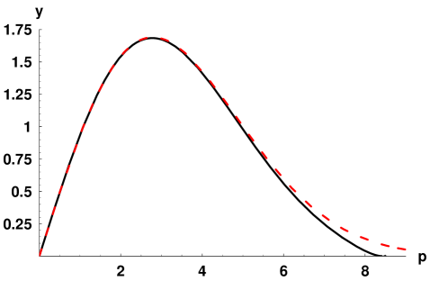
Figure 2: Momentum-space wave function $y(p)$ of Fig. 1(a) resulting from consideration of only 15 terms in its polynomial approximation (25) [full line], in comparison with the corresponding exact ground-state wave function of the relativistic harmonic-oscillator operator [dashed line].

The minimum number of terms to be taken into account in the Taylor-series expansions (23) required in order to achieve some given precision of one’s results will depend, of course, on both the bound state under study and the desired accuracy. From our above remarks we feel entitled to conclude that a reasonable (and manageable) number $N\simeq 40$ produces satisfactory results.

To our knowledge, at present the best semianalytical upper and lower bounds to the energy eigenvalues of the relativistic harmonic-oscillator problem are provided simultaneously by the combination of minimum–maximum principle with operator inequalities [18] and the envelope theory [19, 21]: at least for the relativistic harmonic oscillator the envelope bounds [19, 21] may be shown [23] to be quantitatively equivalent to the bounds derived in Appendix A of Ref. [18]. However, a discussion, in full generality, of all implications of such operator inequalities for the eigenvalues of the operators considered appears clearly off the mainstream of our presentation. Therefore, as already promised in the Introduction, the general relationship is demonstrated in Appendix A. The bounds we need here are derived from this general theorem by specializing to the case of the relativistic harmonic-oscillator problem posed by the Hamiltonian operator (2); all operator inequalities required by this procedure may be generated by, e. g., envelope theory. For a bound state of vanishing relative orbital angular momentum $\ell,$ that is, for a purely radial excitation, identified by the radial quantum number $n_{\rm r}=0,1,2,\dots$ (identical to the number of nodes of the corresponding wave function), the bounds on the dimensionless eigenvalue $\varepsilon$ read

$$\min_{r>0}\left(\sqrt{\mu^{2}+\frac{P_{\rm L}^{2}}{r^{2}}}+r^{2}\right)\leq\varepsilon\leq\min_{r>0}\left(\sqrt{\mu^{2}+\frac{P_{\rm U}^{2}}{r^{2}}}+r^{2}\right),$$

where, in three spatial dimensions, our envelope-theory upper-bound parameter $P_{\rm U}$ is given by

$$P_{\rm U}=2\,n_{\rm r}+\frac{3}{2}\ ,\quad n_{\rm r}=0,1,2,\dots\ ,$$

while the lower-bound parameter $P_{\rm L}$ required for our envelope bounds is related to the zeros $z_{0}$ of Airy’s function ${\rm Ai}(z)$ [47] ($-z_{0}=2.338107,\,4.087949,\,5.520560,\,6.786708,\,7.944134,\,\dots$) by

$$P_{\rm L}=2\left(\frac{-z_{0}}{3}\right)^{3/2}\ ,\quad{\rm Ai}(z_{0})=0\ .$$

Resulting values of $P_{\rm L}$ for the lowest-lying $\ell=0$ bound states are listed in Table 2 [19, 21, 22, 23, 9].

Table 2: Numerical values of the parameter $P_{\rm L}$ used by envelope theory for the lower bounds on the energy levels of the relativistic harmonic-oscillator problem in three spatial dimensions, for the lowest-lying $\ell=0$ bound states identified by their radial quantum number $n_{\rm r}=0,1,2,\dots.$

$n_{\rm r}$	$P_{\rm L}$
0	1.3760835
1	3.1813129
2	4.9925543
3	6.8051369
4	8.6182269

Table 3 compares, for the lowest four $\ell=0$ energy levels (identified by their radial quantum number $n_{\rm r}=0,1,2,3$) of our Hamiltonian (2), the approximate eigenvalues, $\varepsilon(N),$ obtained by the present approach by a truncation of the power series (25) to $N=14$ or $N=44$ terms, with the corresponding semianalytical upper ($\varepsilon_{\rm U}$) and lower ($\varepsilon_{\rm L}$) bounds mentioned above as well as with the (numerically exact) eigenvalues $\varepsilon_{\rm num},$ computed by a method developed for the purely numerical solution of (nonrelativistic) Schrödinger equations [46]. For $N=14,$ the polynomial in $\varepsilon$ resulting from the suitably adapted boundary condition (24) has only two real roots at all. Moreover, both of these approximate values are still above our (semianalytical) upper bounds. In contrast to this rather crude approximation, for $N=44$ the eigenvalues $\varepsilon(N)$ of already the three lowest energy levels fit perfectly to the ranges spanned by the semianalytical bounds. For the ground state, in particular, $\varepsilon(44)$ reproduces the exact result at least to five decimal places.

Table 3: “Compact-origin” eigenvalues $\varepsilon(N),$ their upper ($\varepsilon_{\rm U}$) and lower ($\varepsilon_{\rm L}$) bounds, and their exact values $\varepsilon_{\rm num}$ for the lowest $\ell=0$ states of the Hamiltonian $H/a^{1/3}$ in Eq. (2), with $\mu=30.$

Radial Excitation $n_{\rm r}$	0	1	2	3
$\varepsilon_{\rm U}-\mu$	0.38668	0.90032	1.41179	1.92111
$\varepsilon_{\rm L}-\mu$	0.35478	0.81862	1.28222	1.74440
$\varepsilon_{\rm num}-\mu$	0.38627	0.89857	1.40768	1.91366
$\varepsilon(N=14)-\mu$	0.38854	0.93616	—	—
$\varepsilon(N=44)-\mu$	0.38627	0.89864	1.41032	1.94319

4 Summary and Conclusions

Our compact result for the reduced $\ell=0$ eigenfunctions of the Hamiltonian (2) is given by the power series (23), with expansion coefficients $c_{1}=1,$ $c_{3}=\mu-\varepsilon,$ and $c_{2n+1},$ $n\geq 2,$ determined by the recurrence relation (22). Both the numerical determination of all energy eigenvalues and the explicit construction of the corresponding eigenfunctions of the relativistic harmonic-oscillator problem is then achieved by forcing our solutions to satisfy, in addition, the constraint imposed by the requirement of normalizability of bound-state wave functions. Comparing these explicit solutions with the outcomes of purely numerical integration procedures reveals that at least for the lowest-lying energy levels our semianalytical approach reproduces, already for a truncation of the Taylor series (23) to a moderate number of expansion terms, the exact solutions with high accuracy. Of course, if one is interested only in numerical solutions of the problem under study, their straightforward computation with the help of some integration algorithm should produce the desired result more easily than their extraction from our Taylor series by means of Eq. (24).

Appendix A Combination of minimum–maximum principle with operator inequality: “spectral comparison theorem”

It is a simple exercise to relate discrete eigenvalues of two operators satisfying some inequality.

Consider for some operator $A,$ with domain ${\cal D}(A),$ its eigenvalue equation $A\,|\alpha_{k}\rangle=a_{k}\,|\alpha_{k}\rangle,$ $k=0,1,2,\dots,$ for its set of eigenstates $\{|\alpha_{k}\rangle,\ k=0,1,2,\dots\},$ corresponding to its eigenvalues

$$a_{k}\equiv\frac{\langle\alpha_{k}|\,A\,|\alpha_{k}\rangle}{\langle\alpha_{k}|\alpha_{k}\rangle}\ ,\qquad k=0,1,2,\dots\ ,$$

and likewise for some operator $B,$ with domain ${\cal D}(B),$ its eigenvalue equation $B\,|\beta_{k}\rangle=b_{k}\,|\beta_{k}\rangle,$ $k=0,1,2,\dots,$ for its set of eigenstates $\{|\beta_{k}\rangle,\ k=0,1,2,\dots\},$ corresponding to its eigenvalues

$$b_{k}\equiv\frac{\langle\beta_{k}|\,B\,|\beta_{k}\rangle}{\langle\beta_{k}|\beta_{k}\rangle}\ ,\qquad k=0,1,2,\dots\ .$$

Assume that both these operators $A$ and $B$ are self-adjoint: $A^{\dagger}=A$, $B^{\dagger}=B.$ This implies that all their eigenvalues are real: $a_{k}^{\ast}=a_{k},$ $b_{k}^{\ast}=b_{k},$ $k=0,1,2,\dots.$ Let these eigenvalues be ordered according to $a_{0}\leq a_{1}\leq a_{2}\leq\cdots,$ $b_{0}\leq b_{1}\leq b_{2}\leq\cdots.$ Consider only the discrete eigenvalues $a_{k}$ of $A$ below the onset of the essential spectrum of the operator $A.$ Assume that the operator $A$ is bounded from below. Assume that the operators $A$ and $B$ are related by an operator inequality of the form $A\leq B,$ which implies that $B$ too is bounded from below. In order to derive, for any $k=0,1,2,\dots,$ the relationship between $a_{k}$ and $b_{k},$ focus on some arbitrary $(k+1)$-dimensional subspace $D_{k+1}$ of the domain ${\cal D}(A)$ of $A$: $D_{k+1}\subseteq{\cal D}(A).$ Employing the appropriate form of the minimum–maximum principle, the operator inequality $A\leq B$ translates into an upper bound on the eigenvalue $a_{k}$ of $A$ which involves all expectation values of $B$ within this subspace $D_{k+1}$:

$$a_{k}\leq\sup_{|\psi\rangle\in D_{k+1}}\frac{\langle\psi|\,A\,|\psi\rangle}{\langle\psi|\psi\rangle}\leq\sup_{|\psi\rangle\in D_{k+1}}\frac{\langle\psi|\,B\,|\psi\rangle}{\langle\psi|\psi\rangle}\qquad\mbox{for all}\ k=0,1,2,\dots\ .$$ (26)

Now, in order to relate the supremum over the expectation values of $B$ to the eigenvalues $b_{k}$ of $B,$ consider a particular subspace $D_{k+1},$ namely, that space that is spanned by the first $k+1$ eigenvectors of the operator $B,$ that is, by precisely those eigenvectors of $B$ that correspond to the first $k+1$ eigenvalues $b_{0},b_{1},\dots,b_{k}$ of $B$: $D_{k+1}\subseteq{\cal D}(B)\subseteq{\cal D}(A).$ Then, clearly, every $|\psi\rangle$ in $D_{k+1}$ is a linear combination of the eigenstates $\{|\beta_{i}\rangle,\ i=0,1,\dots,k\}$ of $B,$ with coefficients $c_{i}$:

$$|\psi\rangle=\sum_{i=0}^{k}c_{i}\,|\beta_{i}\rangle\qquad\mbox{for all}\ |\psi\rangle\in D_{k+1}\ .$$

For any subspace $D_{k+1},$ $k=0,1,2,\dots,$ use of this expansion of $|\psi\rangle$ yields for its norm squared

$$\langle\psi|\psi\rangle=\sum_{i=0}^{k}|c_{i}|^{2}\,\langle\beta_{i}|\beta_{i}\rangle\qquad\mbox{for all}\ |\psi\rangle\in D_{k+1}$$

and, with this and $b_{i}\leq b_{k}$ for all $i=0,1,\dots,k,$ an upper bound on all expectation values of $B$:

$$\langle\psi|\,B\,|\psi\rangle=\sum_{i=0}^{k}|c_{i}|^{2}\,b_{i}\,\langle\beta_{i}|\beta_{i}\rangle\leq b_{k}\,\sum_{i=0}^{k}|c_{i}|^{2}\,\langle\beta_{i}|\beta_{i}\rangle=b_{k}\,\langle\psi|\psi\rangle\qquad\mbox{for all}\ |\psi\rangle\in D_{k+1}\ ,$$

which means

$$\frac{\langle\psi|\,B\,|\psi\rangle}{\langle\psi|\psi\rangle}\leq b_{k} \mbox{for all}\ |\psi\rangle\in D_{k+1}\ ,$$

$$\frac{\langle\psi|\,B\,|\psi\rangle}{\langle\psi|\psi\rangle}=b_{k} \mbox{for}\ |\psi\rangle=|\beta_{k}\rangle\in D_{k+1}\ .$$

Therefore the supremum of all expectation values of $B$ over $D_{k+1}$ is just the eigenvalue $b_{k}$ of $B$:

$$\sup_{|\psi\rangle\in D_{k+1}}\frac{\langle\psi|\,B\,|\psi\rangle}{\langle\psi|\psi\rangle}=b_{k}\qquad\mbox{for all}\ k=0,1,2,\dots\ .$$

Thus, inserting this identity in the chain of inequalities (26) proves that corresponding discrete eigenvalues $a_{k},$ $b_{k}$ of semibounded self-adjoint operators $A,$ $B$ that satisfy $A\leq B$ are related by

$$a_{k}\leq b_{k}\qquad\mbox{for all}\ k=0,1,2,\dots\ .$$

References

- [1] E. E. Salpeter and H. A. Bethe, Phys. Rev. 84 (1951) 1232.
- [2] E. E. Salpeter, Phys. Rev. 87 (1952) 328.
- [3] W. Lucha, F. F. Schöberl, and D. Gromes, Phys. Rep. 200 (1991) 127.
- [4] W. Lucha and F. F. Schöberl, Int. J. Mod. Phys. A 7 (1992) 6431.
- [5] W. Lucha and F. F. Schöberl, in: Proc. Int. Conf. on Quark Confinement and the Hadron Spectrum, eds. N. Brambilla and G. M. Prosperi (World Scientific, River Edge (N. J.), 1995) p. 100 [hep-ph/9410221].
- [6] W. Lucha and F. F. Schöberl, in: Proc. XIth Int. Conf. Problems of Quantum Field Theory, eds. B. M. Barbashov, G. V. Efimov, and A. V. Efremov (Joint Institute for Nuclear Research, Dubna, 1999) p. 482 [hep-ph/9807342].
- [7] W. Lucha and F. F. Schöberl, Int. J. Mod. Phys. A 14 (1999) 2309 [hep-ph/9812368].
- [8] W. Lucha and F. F. Schöberl, Fizika B 8 (1999) 193 [hep-ph/9812526].
- [9] W. Lucha and F. F. Schöberl, Recent Res. Devel. Physics 5 (2004) 1423 [arXiv:hep-ph/0408184].
- [10] W. Lucha and F. F. Schöberl, in: Quark Confinement and the Hadron Spectrum VI: 6th Conference on Quark Confinement and the Hadron Spectrum – QCHS 2004, editors: N. Brambilla, U. D’Alesio, A. Devoto, K. Maung, G. M. Prosperi, and S. Serci, AIP Conference Proceedings 756 (American Institute of Physics, 2005) p. 467 [hep-ph/0411069].
- [11] M. Reed and B. Simon, Methods of Modern Mathematical Physics IV: Analysis of Operators (Academic Press, New York, 1978) Sections XIII.1 and XIII.2.
- [12] A. Weinstein and W. Stenger, Methods of Intermediate Problems for Eigenvalues – Theory and Ramifications (Academic Press, New York, 1972) Chapters 1 and 2.
- [13] W. Thirring, A Course in Mathematical Physics 3: Quantum Mechanics of Atoms and Molecules (Springer, New York/Wien, 1990) Section 3.5.
- [14] A. Martin, Phys. Lett. B 214 (1988) 561.
- [15] A. Martin and S. M. Roy, Phys. Lett. B 233 (1989) 407.
- [16] W. Lucha and F. F. Schöberl, Phys. Rev. A 54 (1996) 3790 [hep-ph/9603429].
- [17] W. Lucha and F. F. Schöberl, J. Math. Phys. 41 (2000) 1778 [hep-ph/9905556].
- [18] W. Lucha and F. F. Schöberl, Int. J. Mod. Phys. A 15 (2000) 3221 [hep-ph/9909451].
- [19] R. L. Hall, W. Lucha, and F. F. Schöberl, J. Phys. A 34 (2001) 5059 [hep-th/0012127].
- [20] R. L. Hall, W. Lucha, and F. F. Schöberl, J. Math. Phys. 42 (2001) 5228 [hep-th/0101223].
- [21] R. L. Hall, W. Lucha, and F. F. Schöberl, Int. J. Mod. Phys. A 17 (2002) 1931 [hep-th/0110220].
- [22] R. L. Hall, W. Lucha, and F. F. Schöberl, J. Math. Phys. 43 (2002) 5913 [math-ph/0208042].
- [23] R. L. Hall, W. Lucha, and F. F. Schöberl, Int. J. Mod. Phys. A 18 (2003) 2657 [hep-th/0210149].
- [24] R. L. Hall, W. Lucha, and F. F. Schöberl, in: Proc. Int. Conf. on Quark Confinement and the Hadron Spectrum V, eds. N. Brambilla and G. M. Prosperi (World Scientific, Singapore, 2003) p. 500.
- [25] R. L. Hall, W. Lucha, and F. F. Schöberl, J. Math. Phys. 43 (2002) 1237; ibid. 44 (2003) 2724 (E) [math-ph/0110015].
- [26] R. L. Hall, W. Lucha, and F. F. Schöberl, Phys. Lett. A 320 (2003) 127 [math-ph/0311032].
- [27] R. L. Hall, W. Lucha, and F. F. Schöberl, J. Math. Phys. 45 (2004) 3086 [math-ph/0405025].
- [28] R. J. Duffin, Phys. Rev. 71 (1947) 827.
- [29] M. F. Barnsley, J. Phys. A 11 (1978) 55.
- [30] B. Baumgartner, J. Phys. A 12 (1979) 459.
- [31] J. C. Raynal, S. M. Roy, V. Singh, A. Martin, and J. Stubbe, Phys. Lett. B 320 (1994) 105.
- [32] F. Brau, J. Nonlin. Math. Phys. 12 (2005) S86 [math-ph/0411009].
- [33] W. Lucha, F. F. Schöberl, and M. Moser, arXiv:hep-ph/9401268.
- [34] W. Lucha and F. F. Schöberl, Phys. Rev. A 51 (1995) 4419 [hep-ph/9501278].
- [35] S. Jacobs, M. G. Olsson, and C. Suchyta III, Phys. Rev. D 33 (1986) 3338; ibid. 34 (1986) 3536 (E).
- [36] W. Lucha and F. F. Schöberl, Phys. Rev. D 50 (1994) 5443 [hep-ph/9406312].
- [37] W. Lucha and F. F. Schöberl, Phys. Lett. B 387 (1996) 573 [hep-ph/9607249].
- [38] W. Lucha and F. F. Schöberl, Phys. Rev. A 56 (1997) 139 [hep-ph/9609322].
- [39] W. Lucha and F. F. Schöberl, Phys. Rev. A 60 (1999) 5091 [hep-ph/9904391].
- [40] L. J. Nickisch, L. Durand, and B. Durand, Phys. Rev. D 30 (1984) 660; ibid. 30 (1984) 1995 (E).
- [41] L. Durand and A. Gara, J. Math. Phys. 31 (1990) 2237.
- [42] W. Lucha, H. Rupprecht, and F. F. Schöberl, Phys. Rev. D 45 (1992) 1233.
- [43] L. P. Fulcher, Z. Chen, and K. C. Yeong, Phys. Rev. D 47 (1993) 4122.
- [44] L. P. Fulcher, Phys. Rev. D 50 (1994) 447.
- [45] W. Lucha and F. F. Schöberl, Int. J. Mod. Phys. C 11 (2000) 485 [hep-ph/0002139].
- [46] W. Lucha and F. F. Schöberl, Int. J. Mod. Phys. C 10 (1999) 607 [hep-ph/9811453].
- [47] Handbook of Mathematical Functions, eds. M. Abramowitz and I. A. Stegun (Dover, New York, 1964).