Abstract

We derive an evolution equation for the generating functional which accounts for processes for both gluon emission and recombination. In terms of color dipoles, the kernel of this equation describes evolution as a classical branching process with conserved probabilities. The introduction of dipole recombination allows one to obtained closed loops during the evolution, which should be interpreted as Pomeron loops of the BFKL Pomerons. In comparison with the emission, the dipole recombination is formally $1/N_{c}^{2}$ suppressed. This suppression, nevertheless, is compensated at very high energies when the scattering amplitude tends to its unitarity bound.

1 Introduction

As has been shown by Mueller [1], the high energy scattering in QCD can be treated in the most economical way in terms of color dipole degrees of freedom. In this approach, one considers a fast moving particle, as a system of colorless dipoles. The wavefunction of this system of dipoles can be found from the QCD generating functional [1]. As was shown in Ref. [2, 3] this functional obeys a linear functional evolution equation (see also Ref. [4]). This linear functional evolution equation was derived in large $N_{c}$ approximation. For a small projectile, for which we can neglect nonlinear effects associated with high dipole densities in its wavefunction, the functional evolution was shown to reproduce the dipole version of the Balitsky hierarchy [5] for the scattering amplitude. The latter reduces to the Balitsky-Kovchegov (BK) equation [5, 6] if in addition we assume that the low energy dipole interaction with the target has no correlations.

Though the BK equation has been widely used for phenomenology [7], it is clear starting from the first papers on non-linear collective effects at high energies (see Refs. [8, 9, 10]) that simple non-linear evolution equations of the BK type could be correct only in a very limited kinematic range. At present there are several approaches allowing one to go beyond the BK equation. Balitsky [5] has developed a Wilson line approach which allows the incorporation of both target correlations and $N_{c}$ corrections. This method is equivalent to the effective Lagrangian approach describing the Color Glass Condensate and its derivative JIMWLK equation [11].

The methods above describe high energy evolution in a highly asymmetric manner: either the projectile or target is always considered as a small perturbative probe. Thus, the constructed evolution contains a one way parton shower, in apparent violation of the $t$ channel unitarity [12]. Is is thus challenging to attempt to restore the symmetry of the QCD evolution. If we are successful, we would be able to confront problems of high energy scattering of hadrons or heavy nuclei in a reliable manner.

Several steps have been made recently in attempt to formulate a symmetric evolution. Braun [13] used the QCD triple Pomeron vertex [14] both for Pomeron splittings and mergings. Iancu and Mueller suggested a high energy factorization [12, 15, 16], while a statistical approach to high energy scattering was proposed in Ref. [17]. In its turn, Balitsky in Ref. [18] considered a symmetric scattering of two shock waves. Another technique is due to Lipatov (e.g. [19]) who built an effective theory for reggeized gluons. Unfortunately, a relation between Lipatov‘s theory and the other methods is so far not clear. We want also to restore a symmetry without loosing the probabilistic interpretation of our results which leads to a simplest physical picture of the process and a direct application for experimental observations.

A symmetric way to describe high energy QCD does exist: it is the Reggeon technique [8, 9, 14, 20] based on interacting BFKL Pomerons [21]. Many elements of this technique are known (see Refs. [14, 20]) and the main problem is to sum all Reggeon graphs. Past experience in summing Reggeon diagrams does not look encouraging. However, a remarkable breakthrough was achieved in the last days of the Pomeron approach to strong interactions: it turns out that the Reggeon calculus can be re-written in a probabilistic language. It was possible to formulate equations for probabilities to find a definite number of Pomerons at fixed rapidity [22, 23, 24]. The goal of this paper is to re-write the reggeon calculus of the BFKL Pomerons, by extending our linear functional approach based on dipole generating functional [2, 3]. Colorless dipoles play two different roles in our approach. First, they are partons for the BFKL Pomeron. This role of the dipoles is not related to the large $N_{c}$ approximation. Instead of defining a probability to find Pomerons we search for a probability to find a definite number of dipoles at fixed rapidity. In this approach each vertex for splitting of one Pomeron into two Pomerons can be viewed as a decay of one dipole into two. Vise versa, merging of two Pomerons is an annihilation process of two dipoles into one.

The second role of the color dipoles is that at high energies they are good degrees of freedom. This fact allows us to calculate splitting and merging vertices. However, we need to stress that the dipole model has been proven in the leading large $N_{c}$ approximation only. The main assumption of this paper is that the dipole degrees of freedom can be in fact used for calculation of Pomeron vertices even beyond large $N_{c}$.

Using this assumption we derive, in addition to previously known dipole splitting vertex $\Gamma(1\rightarrow 2)$, two new vertices. The first one stands for the dipole recombination vertex $\Gamma(2\rightarrow 1)$. This vertex is derived by computing a lowest order loop diagram and it is essentially the same as the triple BFKL Pomeron vertex [14, 20]. The only difference is in the normalization which allows us to use this vertex within the framework of the generating functional approach.

The second new vertex is $\Gamma(2\rightarrow 3)$, which accounts for the possibility of a dipole “swing”. What we mean is that with some probability two quarks of a pair of dipoles can exchange their antiquarks to form another pair of dipoles. Naturally, this process has $1/N_{c}^{2}$ suppression. It is the vertex $\Gamma(2\rightarrow 3)$ that correctly accounts for the Pomeron pairwise interaction in the BKP equation [25] and is absent in the usual form of the dipole evolution.

We observe several advantages of our approach based on the generating functional.

• Using the generating functional, we can separate the structure of the wavefunction of the produced dipole at high energy from rather complicated interaction of dipoles with the target at low energy. The latter are subject to non-perturbative QCD calculation and at the moment can be modeled only;

• Our approach is based on colorless dipoles as the correct degrees of freedom at high energy. This fact allows us to have a natural description of hard processes in perturbative QCD, reproducing linear evolution equations, such as DGLAP [26] or/and BFKL [21] equations;

• In our derivation of the linear functional equation we used a method which is closely related to the probabilistic interpretation of the Reggeon Calculus (see Refs. [22, 23, 24]). In doing so we establish a clear correspondence between the color dipole approach to high energy scattering, and Reggeon-like diagram technique providing a natural matching with high energy phenomenology of soft processes based on Pomeron.

In the next section we describe the general formalism of the generating functional and its evolution equation taking into account both the emission of dipoles and their recombination. We also derive the equations for the scattering amplitudes which solve the problem of summation of the BFKL Pomeron loops. In section 3 and in the appendix we discuss the dipole vertices for the process of transition of two dipoles into one. Pomeron interactions via two to three dipole decay is a subject of Section 4. Section 5 is devoted to study of dynamic correlations between dipoles. In conclusions we summarize and discuss our results.

2 Dipole branching and Generating functional

2.1 Classical branching process and equation for probabilities.

We first consider a generic fast moving projectile whose wavefunction can be expended in a dipole basis. Note that contrary to many previous studies, we do not restrict ourselves to a single dipole as a projectile.

$$\Psi^{proj}\,=\,\sum_{n}\,\alpha_{n}\,|n\rangle$$ (2.1)

Let us define a probability density $P_{n}\,=\,\alpha_{n}^{2}$ to find $n$ dipoles with coordinates $r_{1},b_{1}$, $r_{2},b_{2}$, $\dots r_{i},b_{i}$, $\dots\,r_{n},b_{n}$ and rapidity $Y$ in the projectile wavefunction. $r_{i}$ and $b_{i}$ are correspondingly the dipole’s size and impact parameter, both are two dimensional vectors. We define $P_{n}$ as a dimensionfull quantity which gives the probability to find a dipole with the size $r_{i}$ (from $r_{i}$ to $r_{i}+dr_{i}$). The integral

$$\int\,\prod d^{2}r_{i}\,\,P_{n}\left(Y\,-\,Y_{0};\,r_{1},b_{1},\,r_{2},b_{2},\dots r_{n},b_{n}\right)\,\,=\,\,\Pi_{n}$$ (2.2)

and it gives the probability to find $n$-dipole with any sizes. This probability is conserved: $\sum_{n}\Pi_{n}=1$.

Suppose that the following processes can occur as a result of one step in the evolution:

1. The decay of a dipole with the size $r$ and impact parameter $b$ into two dipoles of the sizes $r^{\prime}_{1}$ and $r^{\prime}_{2}$ and impact parameters $b^{\prime}_{1}$ and $b^{\prime}_{2}$ , respectively:

   $$\Gamma(1\rightarrow 2)\equiv\Gamma_{1\rightarrow 2}\left(r,b\,\rightarrow\,r^{\prime}_{1},b^{\prime}_{1}\,+\,r^{\prime}_{2},b^{\prime}_{2}\right)\equiv\Gamma_{1\rightarrow 2}\left(1;\,1^{\prime}\,2^{\prime}\right).$$ (2.3)

2. The annihilation of two dipoles with sizes $r_{1}$ and $r_{2}$ and impact parameters $b_{1}$ and $b_{2}$ into one dipole with the size $r^{\prime}$ and impact parameter $b^{\prime}$:

   $$\Gamma(2\rightarrow 1)\equiv\Gamma_{2\rightarrow 1}\left(r_{1},b_{1}\,+\,r_{2},b_{2}\,\rightarrow\,r^{\prime},b^{\prime}\right)\equiv\Gamma_{2\rightarrow 1}(1\,2;\,1^{\prime}).$$ (2.4)

3. The process of interaction of two dipoles with sizes $r_{1}$ and $r_{2}$ with a creation of one additional dipole (not factorisable to $\Gamma(1\rightarrow 2)$ plus spectator):

   $$\Gamma(2\rightarrow 3)\equiv\Gamma_{2\rightarrow 3}\left(r_{1},b_{1}\,+\,r_{2},b_{2}\,\rightarrow\,r^{\prime}_{1},b^{\prime}_{1}\,+\,r^{\prime}_{2},b^{\prime}_{2}\,+r^{\prime}_{3},b^{\prime}_{3}\,\right)\equiv\Gamma_{2\rightarrow 3}(1\,2\,;\,1^{\prime}\,2^{\prime}\,3^{\prime}).$$ (2.5)

4. The annihilation process of three dipoles into two dipoles:

   $$\Gamma(3\rightarrow 2)\equiv\Gamma_{3\rightarrow 2}\left(r_{1},b_{1}\,+\,r_{2},b_{2}\,+r_{3},b_{3}\,\rightarrow\,r^{\prime}_{1},b^{\prime}_{1}\,+\,r^{\prime}_{2},b^{\prime}_{2}\right)\equiv\Gamma_{3\rightarrow 2}(1\,2\,3\,;\,1^{\prime}\,2^{\prime}).$$ (2.6)

In the remaining of this Section and in the next one we will focus on the first two vertices only. We will discuss $2\leftrightarrow 3$ transition in Section 4.

The equation for $P_{n}$ obeys the classical branching process:

$$\frac{\partial\,P_{n}\left(Y\,-\,Y_{0};\,r_{1},b_{1},\,r_{2},b_{2},\dots r_{n},b_{n}\right)}{\partial\,Y}\,=\,-\,\sum^{n}_{i=1}\,\int\,dV_{f}\,\Gamma_{1\rightarrow 2}\left(i;\,1^{\prime}\,2^{\prime}\right)P_{n}\left(\dots\,r_{i},b_{i}\,\dots\right)$$ (2.7)

$$+\,\sum^{n-1}_{i=1}\,\int dV_{i}\,\Gamma_{1\rightarrow 2}\left(i^{\prime};\,i\,n\right)\,P_{n-1}\left(\dots r^{\prime}_{i},b^{\prime}_{i},\dots\right)-\sum_{i\neq k}\int dV_{f}\,\Gamma_{2\rightarrow 1}\left(i\,k\,;1^{\prime}\right)\,\,P_{n}\left(\dots\,r_{i},b_{i},\dots\right)$$

$$+\,\sum_{i\neq k}\int dV_{i}\,\Gamma_{2\rightarrow 1}\left(i^{\prime}\,k^{\prime};\,i\right)\,\,P_{n+1}\left(\dots\,r^{\prime}_{i},b^{\prime}_{i}\,\dots\,r^{\prime}_{k},b^{\prime}_{k}\dots\right)$$

Eq. (2.7) gives the general evolution for the probabilities $P_{n}$. Eq. (2.7) must be supplemented by explicit expressions for the vertices $\Gamma(1\,\rightarrow\,2)$, $\Gamma(2\,\rightarrow\,1)$. By now, only the vertex $\Gamma(1\,\rightarrow\,2)$ has been calculated in Ref. [1]. On one hand, all other vertices are formally suppressed by $1/N_{c}$ and were omitted being considered as small. Moreover these vertices do not appear at all within the original formulation of the dipole model. On the other hand, it should be stressed that the Feynman diagrams which correspond to these vertices have the same order of magnitude as far as the $N_{c}$ counting is concerned. For example, two diagrams in Fig. 1 show the Born approximation for $\Gamma(1\,\rightarrow\,2)$ (Fig. 1-b ) and for $\Gamma(2\,\rightarrow\,1)$ (Fig. 1-a ). They have the same suppression in $N_{c}$ ($\approx 1/N^{4}_{c}$) but in the diagram of Fig. 1-b this suppression could be absorbed in the amplitude of the interaction of two dipoles with the target while in Fig. 1-a a factor $1/N^{2}_{c}$ has to be assigned to the vertex $\Gamma(2\,\rightarrow\,1)$.

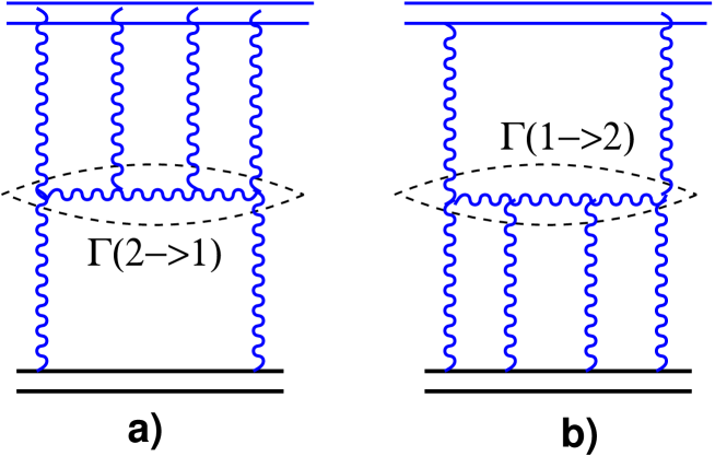
Figure 1: The lowest order diagrams for $\Gamma(2\,\rightarrow\,1)$ (Fig. 1-a) and for $\Gamma(1\,\rightarrow\,2)$ (Fig. 1-b) .

Eq. (2.7) has a very simple structure. For every process of dipole splitting or merging there are two terms: the first one, with the negative sign, accounts for the probability $P_{n}$ to decreases due to splitting or merging of one of $n$ dipoles into dipoles of arbitrary sizes and impact parameters; the second term, with the positive sign, is responsible for an increase in probability to find $n$ dipoles due to the very same processes. The first term includes the vertex $\Gamma(n\rightarrow k)$ integrated over the phase space of the final dipole: $\int\,dV_{f}\,\Gamma(n\rightarrow k)=\int\,\prod^{k}_{l}\,d^{2}r^{\prime}_{l}\,d^{2}b^{\prime}_{l}\,\Gamma(n\rightarrow k)$. For the second term we need to integrate over the phase space of initial dipoles: $\int\,dV_{i}\,\Gamma(n\rightarrow k)=\int\,\prod^{n}_{l}\,d^{2}r_{l}\,d^{2}b_{l}\,\Gamma(n\rightarrow k)$. Explicit expressions for the vertices $\Gamma$ will be given in the next section.

2.2 Generating functional and linear functional evolution

The hierarchy (2.7) can be resolved by introducing a generating functional $Z$

$$Z\left(Y\,-\,Y_{0};\,[u]\right)\,\equiv\,\sum_{n=1}\,\int\,P_{n}\left(Y\,-\,Y_{0};\,r_{1},b_{1},\,r_{2},b_{2},\dots,r_{i},b_{i},\dots,r_{n},b_{n}\right)\,\prod^{n}_{i=1}\,u(r_{i},b_{i})\,d^{2}\,r_{i}\,d^{2}\,b_{i}$$ (2.8)

where $u(r_{i},b_{i})\equiv u_{i}$ is an arbitrary function of $r_{i}$ and $b_{i}$. It follows immediately from (2.7) that the functional (2.8) obeys the condition: at $u\,=\,1$

$$Z\left(Y\,-\,Y_{0};\,[u=1]\right)\,\,=\,\,1\,.$$ (2.9)

The physical meaning of (2.9) is that the sum over all probabilities is one.

Multiplying Eq. (2.7) by the product $\prod^{n}_{i=1}\,u_{i}$ and integrating over all $r_{i}$ and $b_{i}$, we obtain the following linear equation for the generating functional:

$$\frac{\partial\,Z\,[\,u\,]}{\partial\,Y}\,\,=\,\,\chi\,[\,u\,]\,\,Z\,[\,u\,]\,.$$ (2.10)

Let us introduce the dipole collective coordinate $q$ with the integration measure $d^{4}\,q\,=\,d^{2}\,r\,d^{2}\,b$. The evolution kernel $\chi$ is defined trough the operator vertices $V$

$$\chi[u] = -\,\int\,d^{4}\,q\,V_{1\,\rightarrow\,1}\left(q;\,[u]\right)\ +\int\,d^{4}\,q_{1}\,d^{4}\,q_{2}\,V_{1\,\rightarrow\,2}\left(q_{1};q_{2};\,[u]\right)$$

$$- \int\,d^{4}q_{1}\,d^{4}q_{2}V_{2\,\rightarrow\,2}\left(q_{1};q_{2};[u]\right)\,+\,\int\,d^{4}q^{\prime}V_{2\,\rightarrow\,1}\left(q^{\prime};[u]\right)$$

The functional form of the vertices are related to $\Gamma$‘s.

$$V_{1\,\rightarrow\,1}\left(q,[u]\right)\,\,=\,\,\int\,\,d^{4}\,q_{1}\,d^{4}\,q_{2}\,\Gamma_{1\rightarrow 2}\left(q\,\rightarrow\,q_{1}\,+\,q_{2}\right)\,u(q)\,\frac{\delta}{\delta\,u(q)}.$$ (2.11)

$$V_{1\rightarrow 2}(q^{\prime}_{1};\,q^{\prime}_{2};\,[u])\,\,=\,\int d^{4}\,q\,\Gamma_{1\rightarrow 2}\left(q\,\rightarrow\,q^{\prime}_{1}\,+\,q^{\prime}_{2}\right)\,u(q^{\prime}_{1})\,\,u(q^{\prime}_{2})\,\frac{\delta}{\delta u(q)}\,.$$ (2.12)

$$V_{2\,\rightarrow\,2}\left(q_{1};\,q_{2};[u]\right)\,\,=\,\,\frac{1}{2}\,\int\,\,d^{4}\,q\,\,\Gamma_{2\rightarrow 1}\left(q_{1}\,+\,q_{2}\,\rightarrow\,q\right)\,\,u(q_{1})\,u(q_{2})\,\frac{\delta}{\delta\,u(q_{1})}\,\frac{\delta}{\delta\,u(q_{2})}\,.$$ (2.13)

$$V_{2\,\rightarrow\,1}\left(q;[u]\right)\,\,=\,\,\frac{1}{2}\,\int\,\,d^{4}\,q_{1}\,d^{4}\,q_{2}\,\,\Gamma_{2\rightarrow 1}\left(q_{1}\,+\,q_{2}\,\rightarrow\,q\right)\,\,u(q)\,\frac{\delta}{\delta\,u(q_{1})}\,\frac{\delta}{\delta\,u(q_{2})}\,.$$ (2.14)

The functional derivative with respect to $u(q)=u(r,b)$ plays a role of an annihilation operator for a dipole of the size $r$, at the impact parameter $b$. The multiplication by $u(r,b)$ corresponds to a creation operator for this dipole.

Eq. (2.10) exhibits a quantum mechanical-like structure with the operator $\chi$ viewed as a “Hamiltonian” of the evolution. In Eq. (2.2) $\chi$ is constructed in terms of dipole creation and annihilation operators. The evolution operator $\chi$ describes a two dimensional fully quantum (nonlocal) field theory of interacting dipoles.

2.3 Evolution of dipole densities

The $n$-dipole densities in the projectile $\rho_{n}(r_{1},b_{1},\ldots\,,r_{n},b_{n})$ are defined as

$$\rho_{n}(r_{1},b_{1}\,\ldots\,,r_{n},b_{n})\,=\,\frac{1}{n!}\,\prod^{n}_{i=1}\,\frac{\delta}{\delta u_{i}}\,Z\left([u]\right)|_{u=1}$$ (2.15)

Differentiating Eq. (2.10) $n$ times with respect to $u$ we can obtain a hierarchy of equations for $\rho_{n}$ Refs. [6, 2, 3] and rewrite Eq. (2.7) in the form:

$$\frac{\partial\rho_{n}\left(r_{1},b_{1};\dots;r_{n},b_{n};Y\right)}{\partial\,Y}=\,\sum^{n-1}_{i=1}\int d^{4}q\,\Gamma_{1\,\rightarrow\,2}(q;\,q_{i}\,q_{n})\,\rho_{n-1}\left(\dots q\dots\right)$$ (2.16)

$$+\,2\sum_{i=1}^{n}\,\int\,d^{4}q^{\prime}\,d^{4}q\,\Gamma_{1\rightarrow 2}(q^{\prime};qq_{i})\,\rho_{n}\left(\dots q^{\prime}\dots\right)\,-\sum_{i=1}^{n}\int d^{4}q_{1}^{\prime}\,d^{4}q_{2}^{\prime}\,\Gamma_{1\rightarrow 2}(q_{i};q_{1}^{\prime}q_{2}^{\prime})\,\rho_{n}\left(\dots q_{i}\dots\right)$$

$$-\sum^{n}_{i,k,i\neq k}\,\int\,d^{4}\,q\,\Gamma_{2\,\rightarrow\,1}\left(q_{i}\,q_{k};\,q\right)\,\rho_{n}\left(\dots,q_{i},\dots q_{k}\,\dots\right)$$

$$-\,2\,\sum_{i=1}^{n}\,\int d^{4}q\,d^{4}q^{\prime}\Gamma_{2\rightarrow 1}\left(qq_{i};q^{\prime}\right)\,\rho_{n+1}\left(\dots q_{i}\dots q\right)\,+\,\sum_{i=1}^{n}\int\prod^{2}_{i=1}d^{4}q^{\prime}_{i}\,\Gamma_{2\rightarrow 1}\left(q^{\prime}_{1}q^{\prime}_{2};q_{i}\right)\,\rho_{n+1}\left(q^{\prime}_{1}\dots q^{\prime}_{2}\right)$$

Eq. (2.16) presents a general structure with so far arbitrary vertices $\Gamma(1\rightarrow 2)$ and $\Gamma(2\rightarrow 1)$. Explicit expressions for $\Gamma$ will be presented in the next section. The diagonal part of the evolution due to the vertex $\Gamma(1\rightarrow 2)$ is the large $N_{c}$ limit of the BKP equation [25] in coordinate space. $n=1$ corresponds to the evolution of the BFKL Pomeron.

The vertex $\Gamma(2\rightarrow 1)$ (Eq. (3.30)) obeys the following property $\int d^{4}q\,\Gamma_{2\,\rightarrow\,1}\left(q_{i}\,q_{k};\,q\right)\,=\,0$ . Consequently, it is only the last term proportional to $\Gamma(2\rightarrow 1)$ who survives in Eq. (2.16).

2.4 Scattering amplitude

As was shown in Refs. [6, 3], the scattering amplitude is defined as a functional

$$N\left(Y;[\gamma_{i}]\right)=-\sum^{\infty}_{n=1}\,\frac{(-1)^{n}}{n!}\,\int\,\gamma_{n}(r_{1},b_{1};\dots r_{n},b_{n};Y_{0})\,\,\prod^{n}_{i=1}\,\frac{\delta}{\delta u_{i}}Z\left(Y,[u_{i}]\right)|_{u_{i}=1}d^{2}r_{i}\,d^{2}b_{i}\,$$

$$=-\sum^{\infty}_{n=1}(-1)^{n}\,\int\,\gamma_{n}(r_{1},b_{1};\dots r_{n},b_{n};Y_{0})\,\rho_{n}\left(r_{1},b_{1};\dots r_{n},b_{n};Y_{0}\right)\,\prod_{i=1}^{n}\,d^{2}r_{i}\,d^{2}b_{i}\,.$$ (2.17)

The amplitude for simultaneous scattering of $n$ dipoles off the target is denoted by $\gamma_{n}$. It has to be specified at the lowest rapidity ($Y_{0}$). Using the ansatz $N\left((Y,[\gamma_{i}]\right)=N\left(\gamma_{1}(Y),\gamma_{2}(Y)\,\dots\gamma_{i}(Y)\dots\right)$ and having

$$\frac{\partial\,N}{\partial\,Y}=\,\sum^{\infty}_{n=1}\,\int\,\prod^{n}_{i=1}\,d^{2}\,r_{i}\,d^{2}b_{i}\,\,\frac{\delta\,N}{\delta\gamma_{n}}\,\,\frac{\partial\,\gamma_{n}}{\partial\,Y}$$ (2.18)

we can recast the hierarchy of equations (2.16) into the Balitsky-type chain for the scattering amplitudes (see Ref. [3])

$$\frac{\partial\,\gamma_{n}\left(r_{1},b_{1},\dots,r_{n},b_{n}\right)}{\partial\,Y}\,\,\,\,=$$

$$= 2\,\sum_{i=1}^{n}\,\int\,d^{4}q^{\prime}\,d^{4}q\,\Gamma_{1\,\rightarrow\,2}(q_{i};\,q\,q^{\prime})\,\gamma_{n}\left(\dots q^{\prime}\dots\right)\,-\,\sum_{i=1}^{n}\,\int d^{4}q_{1}^{\prime}\,d^{4}q_{2}^{\prime}\,\Gamma_{1\,\rightarrow\,2}(q_{i};\,q_{1}^{\prime}\,q_{2}^{\prime})\,\gamma_{n}\left(\dots,q_{i}\dots\right)$$

$$- \sum^{n-1}_{i=1}\int d^{4}q\,d^{4}q^{\prime}\Gamma_{1\,\rightarrow\,2}(q_{i};\,q\,q^{\prime})\,\gamma_{n+1}\left(\dots q\dots q^{\prime}\right)+\,\sum_{i\neq j}^{n}\,\int d^{4}\,q\,\Gamma_{2\,\rightarrow\,1}\left(q_{i}\,q_{j};\,q\right)\gamma_{n-1}\left(q_{i}\dots q_{j}\dots q\right)$$

$$- 2\,\sum_{i=1}^{n}\int d^{4}q\,d^{4}q^{\prime}\Gamma_{2\rightarrow 1}\left(qq_{i};q^{\prime}\right)\,\gamma_{n-1}\left(\dots q_{i}\dots q\right)\,+\,\sum^{n}_{i,k,i\neq k}\,\int d^{4}q\,\Gamma_{2\rightarrow 1}\left(q_{i}q_{k};q\right)\,\gamma_{n}\left(\dots q_{i}\dots q_{k}\dots\right)$$

The great advantage of Eq. (2.4) is the fact that this equation allows us to take into consideration in the most economic way the interaction of low energy dipoles with the target. For example, assuming $\rho_{1}(Y_{0})=\delta^{(2)}\left(\vec{r}\,-\,\vec{r}_{1}\right)\delta^{(2)}\left(\vec{b}\,-\,\vec{b}_{1}\right)$ while $\rho_{n>1}=0$, we obtain that the total amplitude of a single dipole scattering equals to

$$N\left(r,b;Y\right)\,\,\,=\,\,\,\gamma_{1}\left(r,b;Y\right)\,.$$ (2.20)

If we assume the projectile be built out of two dipoles with
$\rho_{2}(Y_{0})\,\,=\,\,\delta^{(2)}\left(\vec{r}\,-\,\vec{r}_{1}\right)\delta^{(2)}\left(\vec{b}\,-\,\vec{b}_{1}\right)\delta^{(2)}\left(\vec{r}^{\,{}^{\prime}}\,-\,\vec{r}_{2}\right)\delta^{(2)}\left(\vec{b}^{\,{}^{\prime}}\,-\,\vec{b}_{2}\right)$ and $\rho_{1}=0$, $\rho_{n>2}=0$ then

$$N\left(r,b;r^{\prime},b^{\prime};Y\right)\,\,\,=\,\,\,\gamma_{2}\left(r,b;r^{\prime}b^{\prime};Y\right)\,.$$ (2.21)

Eq. (2.4) is an evolution hierarchy for dipole amplitudes. Apparently it involves loop processes. The equation is most general for postulated vertices. It has a very similar structure as suggested by Iancu and Triantafyllopoulos in Ref. [27] (Eqs.(6.6) and (6.7) of this paper). In the following section we will present explicit expressions for all $\Gamma$. The exact vertex $\Gamma(2\,\rightarrow\,1)$ found by us (see Eq. (3.30)) does not seem to coincide with the vertex suggested in Ref. [27] in any kinematic region.

In fact, the last two terms in Eq. (2.4) vanish for the vertex $\Gamma(2\,\rightarrow\,1)$ given by Eq. (3.30). Nevertheless we prefer to keep these terms explicitly in the hierarchy Eq. (2.4). The only reason behind keeping them is that in practical applications one may attempt to approximate or simplify the vertex $\Gamma(2\,\rightarrow\,1)$. For an approximate vertex the last two terms might not vanish. Diagrammatically these terms are part of the $4\rightarrow 4$ reggeized gluon transition which may contribute for some kinematics where the underlying probability conservation is important.

3 Dipole vertices

3.1 $\Gamma(1\,\,\rightarrow\,\,2)$

The vertex for the decay of one dipole into two has been derived in Ref. [1]:

$$\Gamma_{1\rightarrow 2}\left(r,b\,\,\rightarrow\,\,r^{\prime}_{1},b^{\prime}_{2}\,+\,r^{\prime}_{2},b^{\prime}_{2}\right)\,\,\,=$$ (3.22)

$$\bar{\alpha}_{S}\frac{r^{2}}{r^{\prime 2}_{1}\,\,r^{\prime 2}_{2}}\,\delta^{(2)}\left(\vec{r}\,-\,\vec{r}^{\,{}^{\prime}}_{1}\,-\,\vec{r}^{\,{}^{\prime}}_{2}\right)\,\,\delta^{(2)}\left(\vec{b}^{\prime}_{1}\,-\,\vec{b}\,+\,\frac{1}{2}\vec{r}^{\prime}_{2}\right)\delta^{(2)}\left(\vec{b}^{\prime}_{2}\,-\,\vec{b}\,-\,\frac{1}{2}\vec{r}^{\prime}_{1}\right)\,.$$

As has been discussed, this vertex leads to reduction of the probability to find $n$ dipoles due to decay into two dipoles of arbitrary sizes. This reduction is related to

$$\bar{\alpha}_{S}\,\omega(r)\,\,\equiv\,\,\int\,dV^{\prime}\,\Gamma_{1\rightarrow 2}\left(r,b\,\,\rightarrow\,\,r^{\prime}_{1},b^{\prime}_{2}\,+\,r^{\prime}_{2},b^{\prime}_{2}\right)\,\,=\,\,\frac{\bar{\alpha}_{S}}{2\,\pi}\,\int_{\rho}\,\frac{r^{2}}{r^{\prime 2}\,(\vec{r}\,-\,\vec{r}^{\prime})^{2}}\,d^{2}\,r^{\prime}$$ (3.23)

where $\bar{\alpha}_{S}=\alpha_{S}N_{c}/\pi$ and $\rho$ is the infrared cutoff. The growth term is proportional to

$$\int\,dV\,\Gamma_{1\rightarrow 2}\left(r,b\,\,\rightarrow\,\,r^{\prime}_{1},b^{\prime}_{2}\,+\,r^{\prime}_{2},b^{\prime}_{2}\right)\,=\,\int\,d^{2}r\,d^{2}b\,\,\Gamma_{1\rightarrow 2}\left(r,b\,\,\rightarrow\,\,r^{\prime}_{1},b^{\prime}_{2}\,+\,r^{\prime}_{2},b^{\prime}_{2}\right)$$ (3.24)

$$\,\,=\,\,\frac{\bar{\alpha}_{S}}{2\,\pi}\,\frac{(\vec{r}^{\prime}_{1}\,+\,\vec{r}^{\prime}_{2})^{2}}{r^{\prime 2}_{1}\,r^{\prime 2}_{2}}\,\delta^{(2)}\left(\vec{b}^{\prime}_{1}\,-\,\vec{b}^{\prime}_{2}\,-\,\frac{1}{2}(\vec{r}^{\prime}_{1}\,+\,\vec{r}^{\prime}_{2})\right)\,.$$

So far, most of the discussions of dipole evolutions were bounded to the vertex $\Gamma(1\rightarrow 2)$ as all other vertices are $1/N^{2}_{c}$ suppressed and were considered as small corrections. Below we will include several new vertices, which are of the order $1/N^{2}_{c}$. These additional vertices give important contributions in the deep saturation region (see Refs. [8, 12, 15, 16, 17] for more detailed discussion of this subject) and hence need to be accounted for. Though we do not pretend to be able to accommodate all of the $N_{c}$ corrections using dipole degrees of freedom, we believe the contributions we aim to include are dominant at high energies.

3.2 $\Gamma(2\,\,\rightarrow\,\,1)$

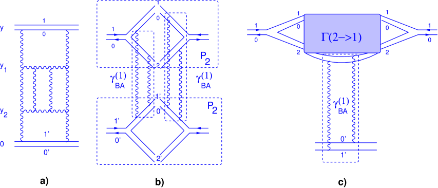
Figure 2: The first enhanced diagram and the vertex of annihilation of two dipoles into one dipole.

To find the vertex $\Gamma(2\to 1)$ we analyze the first enhanced diagram shown in Fig. 2-a. As was shown in Refs. [12, 15] the expression for this diagram is

$$\int\,d^{2}\,r_{1}\,d^{2}\,b_{1}\,\,d^{2}\,r_{2}\,d^{2}\,b_{2}\,\,d^{2}\,r^{\prime}_{1}\,d^{2}\,b^{\prime}_{1}\,d^{2}\,r^{\prime}_{2}\,d^{2}\,b^{\prime}_{2}\,P_{2}\left(r^{\prime}_{1}\,b^{\prime}_{1};r^{\prime}_{2},b^{\prime}_{2}\right)$$

$$\,\,\,\,\,\,\,\,\,\,\,\,\,\,\,\,\,\,\,\,\,\,\,P_{2}\left(r_{1},b_{1};r_{2},b_{2}\right)\,\gamma^{(1)}_{BA}\left(r_{1},r^{\prime}_{1},\vec{b}_{1}\,-\,\vec{b}^{\,{}^{\prime}}_{1}\right)\,\,\gamma^{(1)}_{BA}\left(r_{2},r^{\prime}_{2},\vec{b}_{2}\,-\,\vec{b}^{\,{}^{\prime}}_{2}\right)$$ (3.25)

where $\gamma^{(1)}_{BA}$ is a dipole-dipole elastic scattering amplitude due to exchange of two gluons. The expression for this amplitude is well known (see Refs. [29, 19])

$$\gamma^{(1)}_{BA}\left(r_{1},r^{\prime}_{1};\vec{b}_{1}\,-\,\vec{b}^{\,{}^{\prime}}_{1}\right)\,\,=\,\,\frac{\bar{\alpha}^{2}_{s}}{32\,N_{c}^{2}}\,\,\,\ln^{2}\left(\frac{(\vec{\Delta b}\,+\,\vec{R})^{2}\,(\vec{\Delta b}\,-\,\vec{R})^{2}}{(\vec{\Delta b}\,+\,\vec{\Sigma})^{2}\,(\vec{\Delta b}\,-\,\vec{\Sigma})^{2}}\right)\,\,\equiv\,\,$$ (3.26)

$$\equiv\,\,\frac{\bar{\alpha}^{2}_{S}}{32\,N^{2}_{c}}\,\ln^{2}\left(\frac{(\vec{x}_{1}-\vec{x}^{\,{}^{\prime}}_{1})^{2}\,(\vec{y}_{1}-\vec{y}^{\,{}^{\prime}}_{1})^{2}}{(\vec{x}_{1}-\vec{y}^{\,{}^{\prime}}_{1})^{2}\,\,(\vec{y}_{1}-\vec{x}^{\,{}^{\prime}}_{1})^{2}}\right)$$

where $\vec{\Sigma}\,=\,\frac{1}{2}(\vec{r}_{1}\,+\,\vec{r}^{\,{}^{\prime}}_{1})$, $\vec{R}\,=\,\frac{1}{2}(\vec{r}_{1}\,-\,\vec{r}^{\,{}^{\prime}}_{1})$, $\vec{\Delta b}\,=\,\vec{b}_{1}\,-\,\vec{b}^{\,{}^{\prime}}_{1}$; and $\vec{r}_{1}\,=\,\vec{x}_{1}-\vec{y}_{1}$, $\vec{r}^{\,{}^{\prime}}_{1}\,=\,\vec{x}^{\,{}^{\prime}}_{1}-\vec{y}^{\,{}^{\prime}}_{1}$.

Eq. (3.2) follows from the fact that we can view this diagram in the following way. The upper dipole ($x_{10}$ in Fig. 2) evolves with normal vertex $\Gamma(1\rightarrow 2)$ in the rapidity interval $y-y_{1}$ (see Fig. 2-a) while the low dipole ($x_{1^{\prime}0^{\prime}}$ in Fig. 2) also evolves but in rapidity interval $y_{2}$. As the result of these two evolutions there are two dipoles with the sizes $r_{1}=x_{20}$ and $r_{2}=x_{12}$ at the rapidity $y_{1}$ and two dipoles with sizes $r^{\prime}_{1}=x_{2^{\prime}0^{\prime}}$ and $r_{2}^{\prime}=x_{1^{\prime}2^{\prime}}$ at the rapidity $y_{2}$. Each pair elastically rescatters by the exchange of two gluons leading to Eq. (3.2).

Alternatively, Eq. (2.7) gives another expression for the same diagram

$$\int\,d^{2}\,r_{1}\,d^{2}\,b_{1}\,d^{2}\,r_{2}\,d^{2}\,b_{2}\,\,d^{2}r\,d^{2}\,b\,P_{2}\left(r^{\prime}_{1}\,b^{\prime}_{1}\,r^{\prime}_{2}\,b^{\prime}_{2}\right)\,\Gamma_{2\rightarrow 1}\left(r_{1},b_{1}\,+\,r_{2},b_{2}\rightarrow r,b\right)\gamma^{(1)}_{BA}\left(r,r^{\prime};\vec{b}\,-\,\vec{b}^{\,{}^{\prime}}\right)$$ (3.27)

where $r^{\prime}=x_{1^{\prime}0^{\prime}}$ in Fig. 2. Comparing Eq. (3.2) and Eq. (3.27) we obtain the following equation for $\Gamma_{2\rightarrow 1}\left(r_{1},b_{1}\,+\,r_{2},b_{2}\rightarrow r,b\right)$:

$$\int\,d^{2}\,r\,d^{2}\,b\,\Gamma_{2\rightarrow 1}\left(r_{1},b_{1}\,+\,r_{2},b_{2}\rightarrow r,b\right)\,\gamma^{(1)}_{BA}\left(r,r^{\prime},\vec{b}\,-\,\vec{b}^{\,{}^{\prime}}\right)\,\,=\,\,$$ (3.28)

$$=\,\,\,\int d^{2}\,r^{\prime}_{1}\,d^{2}\,b^{\prime}_{1}\,d^{2}\,r^{\prime}_{2}\,d^{2}\,b^{\prime}_{2}\,\Gamma_{1\rightarrow 2}\left(r^{\prime},b^{\prime}\rightarrow r^{\prime}_{1},b^{\prime}_{1}+r^{\prime}_{2},b^{\prime}_{2}\right)\,\,\gamma^{(1)}_{BA}\left(r_{1},r^{\prime}_{1};\vec{b}_{1}\,-\,\vec{b}^{\,{}^{\prime}}_{1}\right)\,\,\gamma^{(1)}_{BA}\left(r_{2},r^{\prime}_{2},\vec{b}_{2}\,-\,\vec{b}^{\,{}^{\prime}}_{2}\right)\,.$$

Eq. (3.28) is the basic equation from which the vertex $\Gamma(2\rightarrow 1)$ can be extracted. To this goal we need to invert Eq. (3.28) by acting on both sides of it by an operator inverse to $\gamma_{BA}$ in operator sense. Fortunately, this operator is known to be a product of two Laplacians:

$$\Delta_{x}\,\Delta_{y}\,\gamma^{(1)}_{BA}\left(x,y;x^{\prime},y^{\prime}\right)\,\,=\,\,\alpha_{S}^{2}\left(\delta^{(2)}\left({x}-{x}^{\,{}^{\prime}}\right)\delta^{(2)}\left({y}-{y}^{\,{}^{\prime}}\right)\,+\,\delta^{(2)}\left({x}-{y}^{\,{}^{\prime}}\right)\delta^{(2)}\left({y}-{x}^{\,{}^{\prime}}\right)\right)$$ (3.29)

with $x=b+r/2$ and $y=b-r/2$ being the coordinates of quark and antiquark in the dipole $(r,b)$. For the vertex $\Gamma(2\rightarrow 1)$ we finally obtain

$$\Gamma_{2\rightarrow 1}\left(r_{1},b_{1}\,+\,r_{2},b_{2}\rightarrow r,b\right) = \frac{1}{\alpha_{S}^{2}}\,\Delta_{x}\,\Delta_{y}\,\int d^{2}\,r^{\prime}_{1}\,d^{2}\,b^{\prime}_{1}\,d^{2}\,r^{\prime}_{2},d^{2}\,b^{\prime}_{2}\,\Gamma_{1\rightarrow 2}\left(r,b\rightarrow r^{\prime}_{1},b^{\prime}_{1}+r^{\prime}_{2},b^{\prime}_{2}\right)\,\times$$ (3.30)

$$\times \,\gamma^{(1)}_{BA}\left(r_{1},r^{\prime}_{1},\vec{b}_{1}\,-\,\vec{b}^{\,{}^{\prime}}_{1}\right)\,\,\gamma^{(1)}_{BA}\left(r_{2},r^{\prime}_{2};\vec{b}_{2}\,-\,\vec{b}^{\,{}^{\prime}}_{2}\right)\,.$$

In Appendix A we present a method for evaluation of the expression (3.30). We arrive at the result given by Eq. (A.22). Since the general expression is rather complicated we consider now simplified estimates valid in several different kinematic regions.

In the region where $\Delta b\,\ll\,r^{\prime}$ and $r\,\ll\,r^{\prime}$ Eq. (3.26) leads to a simple expression

$$\gamma^{(1)}_{BA}\left(r,r^{\prime};\Delta b\right)\,\,=\,\,\frac{2\bar{\alpha}_{S}^{2}}{N^{2}_{c}}\,\frac{r^{2}}{r^{\,{}^{\prime}2}}$$ (3.31)

Using Eq. (3.31) we can rewrite Eq. (3.28) in the simple form if we are looking for the contribution in the following kinematic region:

$$r_{1}\,\,\approx\,\,r_{2}\,\gg\,r^{\prime}_{1}\,\,\approx\,\,\,r^{\prime}_{2}\,\,\,\,\gg\,\,\,r^{\prime}\,\,\,\,\,\mbox{and}\,\,\,\,r\,\,\gg\,\,r^{\prime}$$

In this kinematic region using Eq. (3.22) and Eq. (2.7) we obtain that the r.h.s. of Eq. (3.28) is equal to

$$\mbox{r.h.s.\,\,of\,\,{Eq.~{}(\ref{G213})}}\,\,\,=\,\,\,\,\bar{\alpha}_{S}\,\,\left(\frac{\bar{\alpha}_{S}}{N^{2}_{c}}\right)^{2}\,\int\,\,d^{2}r^{\prime}_{1}\,d^{2}\,r^{\prime}_{2}\,d^{2}\,b^{\prime}_{1}\,d^{2}b^{\prime}_{2}\,\,$$ (3.32)

$$\left(\gamma^{(1)}_{BA}\left(r_{1},r^{\prime}_{1};\vec{b}_{1}-\vec{b}^{\,{}^{\prime}}_{1}\right)\,=\,\,\frac{r^{\,{}^{\prime}2}_{1}}{r^{2}_{1}}\right)\,\,\left(\gamma^{(1)}_{BA}\left(r_{2},r^{\prime}_{2};\vec{b}_{2}-\vec{b}^{\,{}^{\prime}}_{2}\right)\,=\,\,\frac{r^{\,{}^{\prime}2}_{2}}{r^{2}_{2}}\right)$$

$$\,\frac{r^{\prime 2}}{r^{\,{}^{\prime}2}_{1}\,\,r^{\,{}^{\prime}2}_{2}}\,\,\delta^{(2)}\left(\vec{r}^{\,{}^{\prime}}\,-\,\vec{r}^{\,{}^{\prime}}_{1}\,-\,\vec{r}^{\,{}^{\prime}}_{2}\right)\,\delta^{(2)}\left(\vec{b}^{\,{}^{\prime}}_{1}\,-\,\vec{b}\,+\,\frac{1}{2}\vec{r}^{\,{}^{\prime}}_{2}\right)\,\delta^{(2)}\left(\vec{b}^{\,{}^{\prime}}_{2}\,-\,\vec{b}\,-\,\frac{1}{2}\vec{r}^{\,{}^{\prime}}_{1}\right)\,\,=\,\,$$

$$=\,\,\,\bar{\alpha}_{S}\,\,\left(\frac{\bar{\alpha}_{S}^{2}}{N^{2}_{c}}\,\right)^{2}\,\int\,\,d^{2}\,r^{\prime}_{1}\,\,\frac{r^{\prime 2}}{r^{\,{}^{\prime}2}_{1}\,\,r^{\,{}^{\prime}2}_{2}}\,\frac{r^{\,{}^{\prime}2}_{1}\,\,r^{\,{}^{\prime}2}_{2}}{r^{2}_{1}\,r^{2}_{2}}\,\,=\,\,\,\,\,\bar{\alpha}_{S}\,\,\left(\frac{\,\bar{\alpha}_{S}^{2}}{N^{2}_{c}}\,\right)^{2}\,\frac{r^{\prime 2}}{r^{2}_{1}}$$

The l.h.s of Eq. (3.28) has a form

$$\mbox{l.h.s.\,\,of\,\,{Eq.~{}(\ref{G213})}}\,\,=$$ (3.33)

$$\,\,\frac{32\,\bar{\alpha}_{S}^{2}}{N^{2}_{c}}\,\int\,\,d^{2}r\,d^{2}\,b\,\Gamma_{2\rightarrow 1}\left(r_{1},b_{1}\,+\,r_{2},b_{2}\,\rightarrow\,r,b\right)\left(\gamma^{(1)}_{BA}\left(r,r^{\prime};\vec{b}-\vec{b}^{\,{}^{\prime}}\right)\,=\,\,\frac{r^{2}}{r^{\,{}^{\prime}2}}\right)\,=\,$$

$$=\,\,\frac{32\,\bar{\alpha}_{S}^{2}}{N^{2}_{c}}\pi\int^{r^{2}_{1}}_{r^{\prime 2}}\,\,r^{\prime 2}\,dr^{2}\,\Gamma_{2\rightarrow 1}\left(r_{1},b_{1}\,+\,r_{2},b_{2}\,\rightarrow\,r,b\right)\,$$

In the last equation we used the fact that in Eq. (3.26) the typical $b$ is about the size of the large dipole ($b\,\approx\,r^{\prime}$). Substituting Eq. (3.32) and Eq. (3.33) in Eq. (3.28) we obtain $\Gamma\left(2\,\rightarrow\,1\right)$ in the form

$$\Gamma_{2\rightarrow 1}\left(r_{1},b_{1}\,+\,r_{2},b_{2}\,\rightarrow\,r,b\right)\,\,=\,\,\frac{(4\,\bar{\alpha}_{S})^{3}}{N^{2}_{c}}\,\,\frac{1}{r^{4}_{1}}\,\,$$ (3.34)

Repeating the same calculation but in a different kinematic region:

$$r_{1}\,\approx\,r_{2}\,\ll\,r^{\prime}_{1}\,\,\approx\,r^{\prime}_{2}\,\,\,\mbox{and}\,\,\,r^{\prime}_{1}\,\,\approx\,r^{\prime}_{2}\,\,\gg\,\,r^{\prime}\,\,\,\mbox{while}\,\,\,r\,\,\ll\,\,r^{\prime}$$

we obtain

$$\Gamma_{2\rightarrow 1}\left(r_{1},b_{1}\,+\,r_{2},b_{2}\,\rightarrow\,r,b\right)\,\,=\,\,\frac{(4\,\bar{\alpha}_{S})^{3}}{N^{2}_{c}}\,\,\frac{r^{2}_{1}\,r^{2}_{2}}{r^{8}}$$ (3.35)

The full expression for $\Gamma\left(2\,\rightarrow\,1\right)$ is rather complicated as can be seen from Eq. (A.22). In corresponding limits it reproduces Eq. (3.34) and Eq. (3.35).

4 Pomeron interaction: $2\,\rightarrow 3$ transition vertex

In this section we further extend the dipole model by introducing an additional splitting vertex, $\Gamma(2\rightarrow 3)$. Our main goal here is to account for Pomeron pairwise interactions via exchange of a single gluon. For the first time this process was included in the double log approximation of pQCD in Refs. [30, 31]. It is also most naturally included in the BKP equation [25] providing $1/N_{c}^{2}$ corrections to the dipole evolution discussed above.

The inclusion of the above Pomeron interactions in terms of dipole degrees of freedom is not a straightforward task. We face two problems here. First, the contribution we are looking for is a process in which a gluon is emitted (in the amplitude) by one dipole and then reabsorbed (in the conjugate amplitude) by another dipole. This is an interference contribution, which does not admit a probabilistic interpretation. The exact expression for $N_{c}$ corrections to the dipole evolution known from Refs. [32, 33] can, nevertheless, be projected onto dipole degrees of freedom. By introducing the vertex $\Gamma(2\rightarrow 3)$ we take into account only the diagonal contributions factorisable in terms of dipoles. We trust that the rest of the $N_{c}$ corrections contribute to multi gluon $t$-channel states only. The latter, $n$-gluon states are known to have intercepts smaller than that of $n/2$ Pomerons and thus could be ignored at high energies.

The second problem is in the fact that dipoles are natural degrees of freedom in the large $N_{c}$ limit only. Beyond large $N_{c}$, the dipole basis (2.1) is overcomplete. In particular, a single space configuration of two pairs of quarks and antiquarks can be counted twice as two different pairs of dipoles (provided all quarks are mutually in a color singlet state). As a result of working with overcomplete basis there will be a nontrivial overlap between probabilities to find a different number of dipoles.

Having sorted the above problems out, we propose the following vertex $\chi^{2\rightarrow 3}$ to be added to the dipole evolution kernel $\chi$:

$$\chi^{2\rightarrow 3}\, = \,\int_{x_{1},\,x_{2},\,x_{3}\,x_{4},\,x_{5}}\Gamma_{2\rightarrow 3}\left(x_{2},x_{3},x_{5}\right)\,\,\times$$

$$\times \left[1\,-\,u(x_{1},x_{4})\right]\,\left[u(x_{2},x_{3})\,-\,u(x_{2},x_{5})\,u(x_{5},x_{3})\right]\,\frac{\delta}{\delta\,u(q_{1})}\,\frac{\delta}{\delta\,u(q_{2})}\,.$$

The operator (4) describes the following process. First, it annihilates two dipoles $q_{1}=(x_{1},\,x_{2})$ and $q_{2}=(x_{3},\,x_{4})$ (Fig. 3). Then the dipoles are regrouped into $14$ (spectator) and $23$. The latter subsequently decays through the usual $1\rightarrow 2$ dipole splitting process ($u(x_{1},x_{4})\,(u(x_{2},x_{3})$
$-u(x_{1},x_{4})\,u(x_{2},x_{5})\,u(x_{5},x_{3}))$ term in the operator). The vertex $\Gamma(2\rightarrow 3)$ has the usual dipole splitting form ($\Gamma(1\rightarrow 2)$) suppressed by a factor $N_{c}^{2}$:

$$\Gamma_{2\rightarrow 3}(x,\,y,\,z)\,=\,\frac{\bar{\alpha}_{s}}{2\,\pi\,N_{c}^{2}}\,\frac{(x\,-\,y)^{2}}{(x\,-\,z)^{2}(y\,-\,z)^{2}}$$

In (4) we have also subtracted a term with the spectator $u(x_{1},x_{4})$ set to unity. This subtraction is needed to remove the double counting: the decay of a single dipole ($23$) has been already accounted for in the normal $1\to 2$ dipole evolution. This subtraction can be also thought of as originating from the overcomplete basis we are dealing with. We will find below that this subtraction is crucial to prevent the operator (4) from generating Pomeron loops at the level of scattering amplitudes .

Figure 3: The process $x_{12}+x_{34}\,\rightarrow\,x_{14}+x_{35}+x_{45}$.

For the evolution of the dipole densities $\rho_{n}$ the operator $\chi^{2\rightarrow 3}$ generates the following contribution (for $n\geq 2$)

$$\frac{\partial\rho_{n}\left(q_{1};\dots;q_{n};Y\right)}{\partial\,Y} = \sum_{i,j,k=1,\,i\neq j\neq k}^{n}\,\Gamma_{2\rightarrow 3}(x_{j},y_{k},y_{j})\,\rho_{n-1}(\dots x_{i},y_{k}\dots x_{j},y_{i}\dots)\,\delta^{2}(x_{k}\,-\,y_{j})$$ (4.37)

$$+ \,\sum_{i,j=1,\,i\neq j}^{n}\int d^{2}y\,\Gamma_{2\rightarrow 3}(x_{j},y,y_{j})\,\rho_{n}(\dots x_{i},y\dots x_{j},y_{i}\dots)$$

$$- \,\sum_{i,j=1,\,i\neq j}^{n}\int d^{2}z\,\Gamma_{2\rightarrow 3}(x_{j},y_{j},z)\,\rho_{n}(\dots x_{i},y_{j}\dots x_{j},y_{i}\dots)$$

The evolution of the scattering amplitudes receives additional terms (for $n\geq 2$):

$$\frac{\partial\gamma_{n}\left(q_{1};\dots;q_{n};Y\right)}{\partial\,Y}\,=\sum_{i,j,\,i\neq j}^{n}\,\int d^{2}z\,\Gamma_{2\rightarrow 3}(x_{j},y_{i},z)\left[\gamma_{n}(\dots x_{i},y_{j}\dots x_{j},z\dots)\,+\,\right.$$ (4.38)

$$\gamma_{n}(\dots x_{i},y_{j}\dots z,y_{i}\dots)-\left.\gamma_{n}(\dots x_{i},y_{j}\dots x_{j},y_{i}\dots)\,-\,\gamma_{n+1}(\dots x_{i},y_{j}\dots x_{j},z\dots z,y_{i}\dots)\right]$$

Eq. (4.38) supplemented by the usual dipole evolution generated by the vertex $\Gamma(1\rightarrow 2)$ is believed to be a very good approximation to the Balitsky-JIMWLK evolution. The advantage of our formulation is that it is given entirely in terms of dipole degrees of freedom. We will demonstrate in the following section that the above evolution happens to coincide with the one found in Ref. [34] by analyzing $N_{c}$ corrections arising from the QCD triple Pomeron vertex [14].

Finally let us comment about $3\,\rightarrow 2$ transition vertex. The process of $3\,\rightarrow 2$ has $1/N^{4}_{c}$ compared to the leading $1\,\rightarrow 2$. Indeed, it progresses in two stages: the first one is the annihilation of two dipoles into one. Such a process has $1/N^{2}_{c}$ suppression. Then two remaining dipoles “swing” quarks (see Fig. 3) and this has an additional $1/N_{c}^{2}$ suppression. Therefore, $\Gamma(3\,\,\rightarrow\,\,2)$ is of the order of $1/N^{4}_{c}$ and will be neglected.

5 $N_{c}$ correlations due to $2\,\rightarrow\,3$ vertex

Let us combine Eq. (2.4) and Eq. (4.38) but neglect the vertex $\Gamma(2\,\rightarrow\,1)$. We would like to find a procedure which would allow the equations entering the hierarchy to decouple from each other. In case of original Balitsky‘s hierarchy this was achieved by assuming absence of target correlations which means substitution of the Kovchegov‘s factorization [6]:

$$\gamma_{n}\left(r_{1},b_{1}\,\dots,\,r_{n},b_{n};Y\right)\,\,\,=\,\,\prod^{n}_{i=1}\,\,\gamma_{i}\left(r_{i},b_{i};Y\right)\,.$$ (5.39)

The whole hierarchy respected the factorization leaving only one single equation (BK) unresolved.

Since we have dynamical correlations, the hierarchy of Eq. (2.4)+Eq. (4.38) obviously does not admit the factorization of Eq. (5.39). An intuitive solution would be to introduce pairwise correlations which would hopefully reduce the hierarchy to two coupled equations. The natural generalization of Eq. (5.39) is to introduce two-dipole correlation $C\left(r_{i},b_{i};r_{k},b_{k};Y\right)$ in the form

$$\gamma_{n}\left(r_{1},b_{1}\,\dots,\,r_{n},b_{n};Y\right)\,\,\,=$$ (5.40)

$$\,\,\prod^{n}_{i=1}\,\,\gamma_{i}\left(r_{i},b_{i};Y\right)\,\,\,+\,\,\sum^{n}_{i=1,k=1,i\neq k}\prod^{n}_{l=1,l\neq i,l\neq k}\,\,C\left(r_{i},b_{i};r_{k},b_{k};Y\right)\,\,\gamma_{i}\left(r_{l},b_{l};Y\right)$$

Eq. (5.40) can be written compactly by introducing the operator $Q$, such that

$$\gamma_{n}\left(r_{1},b_{1}\,\dots,\,r_{n},b_{n};Y\right)\,\,\,=Q[\gamma_{1}]\,\,\prod_{i}^{n}\,\gamma_{1}(r_{i},\,b_{i})\,,$$ (5.41)

with

$$Q[\gamma_{1}]\,\,\equiv\,\,Exp\,\left(\int\,d^{4}q_{1}\,d^{4}q_{2}\,C\left(q_{1};\,q_{2};\,Y\right)\,\frac{\delta}{\delta\,\gamma_{1}(q_{1})}\,\frac{\delta}{\delta\,\gamma_{1}(q_{2})}\right)\,.$$

We have checked that, though the introduction of correlations in the form Eq. (5.40) is very plausible idea, this ansatz does not make the system of hierarchy equations to decouple. Nevertheless, we can try to estimate the influence of the new vertex by taking into account the correlations between dipoles in perturbative way considering them small. To this goal we will focus on the first two equations of Eq. (2.4)+Eq. (4.38) which will allow us to determine the evolution law for $\gamma_{1}$ and $C$. Introducing $K$ as the usual dipole kernel

$$K\left({x},{y};{z}\right)\,\,\,=\,\,\frac{({x}-{y})^{2}}{({x}-{z})^{2}\,\,({x}\,-\,{z})^{2}}\,$$ (5.42)

the equations for $\gamma_{1,2}$ read

$$\frac{\partial\,\gamma_{1}\left(x,y\right)}{\partial\,Y}\,=\,\bar{\alpha}_{S}\int_{z}\,K\left({x},{y};{z}\right)\,\left({-\,\gamma_{1}}\left({x},{y}\right)+\,\gamma_{1}\left({x},{z}\right)\,+\,\gamma_{1}\left({y},{z}\right)-\,\gamma_{2}\left({x},{z};{y},{z}\right)\right)\,\,\,\,\,\,\,\,\,\,\,\,\,\,\,$$

(5.43)

$$\frac{\partial\,\gamma_{2}\left(x_{1},y_{1};x_{2},y_{2}\right)}{\partial\,Y}\,=\,$$

$$\,\bar{\alpha}_{S}\,\int_{z}\,\sum_{i,j=1,\,i\neq j}^{2}\,K\left({x_{i}},{y_{i}};{z}\right)\,\left[\gamma_{2}\left({x_{i}},{z};x_{j},y_{j}\right)\,+\,\gamma_{2}\left({y_{i}},{z};x_{j},y_{j}\right){-\,\gamma_{2}}\left({x_{i}},{y_{i}};x_{j},y_{j}\right)\right]$$

$$+\,\,\frac{\bar{\alpha}_{S}}{N_{c}^{2}}\,\int_{z}\sum_{i,j=1,\,i\neq j}^{2}\,K(x_{j},y_{i};z)\,\left[\gamma_{2}(x_{i},y_{j};x_{j},z)\,+\,\right.\gamma_{2}(x_{i},y_{j};z,y_{i})-\left.\gamma_{2}(x_{i},y_{j};x_{j},y_{i})\right]$$

In Eq. (5.43) we have omitted terms proportional to $\gamma_{3}$. Substituting

$$\gamma_{1}\left({x},{y};Y\right)\,\equiv\,N\left({x},{y};Y\right)$$

and

$$\gamma_{2}\left({x}_{1},{y}_{1};{x}_{2},{y}_{2};Y\right)\,=\,N\left({x}_{1},{y}_{1};Y\right)\,\,N\left({x}_{2},{y}_{2};Y\right)\,+\,\,C\left({x}_{1},{y}_{1};{x}_{2},{y}_{2};Y\right)$$

we obtain assuming the correlation function $C$ is small, $C<N^{2}$:

$$\frac{\partial\,N\left({x},{y};Y\right)}{\partial\,Y} = \bar{\alpha}_{S}\int\,d^{2}z\,K\left({x},{y};{z}\right)\,\left({\cal N}\left({x},{y};{z}\right)-\,N\left({x},{z}\right)\,N\left({x},{z}\right)-\,C\left({x},{z};{y},{z};Y\right)\right)=$$ (5.44)

$$= \,\bar{\alpha}_{S}\,\int\,d^{2}\,z\,\,K\left({x},{y};{z}\right)\,\,\left(\tilde{\cal{N}}\left({x},{y};{z}\right)\,\,-\,\,C\left({x},{z};{y},{z};Y\right)\right);$$

where we define

$${\cal N}\left({x},{y};{z}\right)\,\equiv\,N\left({x},{z}\right)\,+\,N\left({y},{z}\right)\,-\,N\left({x},{y}\right)$$ (5.45)

$$\tilde{\cal{N}}\left({x},{y};{z}\right)\,\equiv\,{\cal N}\left({x},{y};{z}\right)\,-\,\,N\left({x},{z}\right)\,N\left({x},{z}\right)$$

$${\,\cal C}\left({x}_{1},{y}_{1},{z};{x}_{2},{y}_{2};Y\right)\,\,\equiv\,\,C\left({x}_{1},{z};{x}_{2},{y}_{2};Y\right)\,+\,C\left({y}_{1},{z};{x}_{2},{y}_{2};Y\right),\,\,-\,\,C\left({x}_{1},{y}_{1};{x}_{2},{y}_{2};Y\right)$$

The equation for $\gamma_{2}$ becomes an equation for $C$

$$\frac{\partial\,C\left({x}_{1}{y}_{1};{x}_{2},{y}_{2};Y\right)}{\partial\,Y}\,\,=$$ (5.46)

$$\,\,\frac{\bar{\alpha}_{S}}{2}\,\int\,d^{2}\,z\,\left(K\left({x}_{1}{y}_{1};{z}\right){\cal{C}}\left({x}_{1},{y}_{1},{z};{x}_{2},{y}_{2};Y\right)\,+\,K\left({x}_{2}{y}_{2};{z}\right)\,\,{\cal{C}}\left({x}_{1},{y}_{1};{x}_{2}{y}_{2},{z};Y\right)\right)$$

$$+\,\,\frac{\bar{\alpha}_{S}}{2\,N^{2}_{c}}\,\left(\int\,d^{2}\,z\,\left(K\left({y}_{1},{x}_{2};{z}\right)\,{\cal{C}}\left({y}_{1},{x}_{2},{z};{x}_{1},{y}_{2};Y\right)\,\,+\,\,\,K\left({x}_{1},{y}_{2};{z}\right){\cal{C}}\left({x}_{1},{y}_{2},{z};{x}_{2},{y}_{1};Y\right)\right)\right.$$

$$\left.+\,\,\int\,d^{2}\,z\,K\left({y}_{1},{x}_{2};{z}\right)\,\left(\,N\left({x}_{1},{y}_{1}\right)\,+\,N\left({x}_{2},{y}_{2}\right)\,-\,N\left({x}_{1},{y}_{2}\right)\,\right)\,\left(\tilde{\cal{N}}\left({y}_{1},{x}_{2};{z}\right)\,+\,\tilde{\cal{N}}\left({x}_{1},{y}_{2};{z}\right)\right)\right)$$

It is interesting to notice that Eq. (5.46) can be reduced to the equation of Bartels, Lipatov and Vacca [34]. Indeed, we can introduce a new function $\Delta C$:

$$\Delta C\left({x}_{1},{y}_{1};{x}_{2},{y}_{2};Y\right)\,\,\,=$$ (5.47)

$$C\left({x}_{1},{y}_{1};{x}_{2},{y}_{2};Y\right)\,\,-\,\,\frac{1}{N^{2}_{c}}\,\left(N\left({x}_{1},{y}_{1};Y\right)\,+\,N\left({x}_{2},{y}_{2};Y\right)\,-\,N\left({x}_{1},{y}_{2};Y\right)\right)^{2}$$

Using Eq. (5.44) we can reduce the set of Eq. (5.44) and Eq. (5.46) to a different set of equations, namely,

$$\frac{\partial\,N\left({x},{y};Y\right)}{\partial\,Y}\,\,=$$ (5.48)

$$\bar{\alpha}_{S}\,\int\,d^{2}\,z\,\,K\left({x},{y};{z}\right)\,\,\left({\cal{N}}\left({x},{y};{z}\right)\,\,-\,\,\,N\left({x},{z}\right)\,N\left({x},{z}\right)-\frac{1}{2\,N^{2}_{c}}{\cal{N}}^{2}\left({x},{y};{z}\right)\,\,+\,\,\Delta C\left({x},{z};{y},{z};Y\right)\right);$$

$$\frac{\partial\,\Delta C\left({x},{z};{y},{z};Y\right)}{\partial\,Y}\,\,=\,\,$$ (5.49)

$$\frac{\bar{\alpha}_{S}}{2}\,\int\,d^{2}\,z\,\left(\,K\left({x}_{2},{y}_{2};{z}\right)\,\,\Delta{\cal{C}}\left({y}_{1},{x}_{2},{z};{x}_{1},{y}_{2};Y\right)\,\,+\,\,\,K\left({x}_{1},{y}_{2};{z}\right)\,\,\Delta{\cal{C}}\left({x}_{1},{y}_{2},{z};{x}_{2},{y}_{1};Y\right)\right)\,+$$

$$\,+\,\,\frac{\bar{\alpha}_{S}}{2\,N^{2}_{c}}\,\int\,d^{2}\,z\,\left(K\left({y}_{1},{x}_{2};{z}\right)N\left({y}_{1},{z};Y\right)\,\,N\left({x}_{2},{z};Y\right)\,\,+\,\,\,K\left({x}_{1},{y}_{2};{z}\right)N\left({y}_{1},{z};Y\right)\,\,N\left({x}_{2},{z};Y\right)\right)$$

These two equations are the same as were proposed by Bartels, Lipatov and Vacca [34]. Our derivation suggests also a physical meaning of the modified Balitsky-Kovchegov equation (see Eq. (5.48)). The Balitsky-Kovchegov equation is a mean field approximation while Eq. (5.48) takes into account the correlation related to possibility for grouping of two dipoles in a different way with suppressed probability. Therefore, it plays a role of Fock term in Hartree-Fock approach, which is a natural next step in the mean field approach. $\Delta C$ is a real dynamic correlations which as one can see from Eq. (5.49) grows with energy. We have neglected terms of the order $\Delta CN$ in comparison with $N^{2}$ -term. Therefore, we can trust the equations only for $\Delta C\leq N$. For higher energies we need to develop a more general approach.

6 Conclusions and Discussion

In this paper we have extended our linear operator approach applied to dipole evolution. The evolution kernel $\chi$ can be viewed as a “Hamiltonian” of the evolution. It is constructed in terms of dipole creation ad annihilation operators. By introducing the recombination vertex $\Gamma\left(2\rightarrow 1\right)$, the evolution operator has been promoted to a fully quantum two dimensional field theory of interacting dipoles (Pomerons).

The main results of this paper are Eq. (2.10), Eq. (2.16), Eq. (2.4), Eq. (4) and Eq. (4.38) supplemented by the explicit expressions for the vertices $\Gamma\left(2\rightarrow 1\right)$ and $\Gamma\left(2\rightarrow 3\right)$ which both are proportional to the second functional derivative with respect to $u_{i}$. Our approach is an extension beyond the Balitsky one [5], based on the Wilson loops, as well as beyond the Color Glass Condensate approach (JIMWLK equation [10, 11]). Though the JIMWLK equation takes into account all $1/N^{2}_{c}$ corrections, and which are only partially accounted for by the vertex $\Gamma(2\rightarrow 3)$, they do not include the recombination vertex $\Gamma(2\rightarrow 1)$ which is a major step beyond this equation.

We have accounted for dynamical correlations that stem from possibility of merging of two BFKL Pomerons. It is illustrative to consider a simple toy model in which we assume that interactions do not depend on the dipole sizes (see Refs. [1, 2, 15] for details). The master functional equation (see Eq. (2.10)) for this model degenerates into ordinary equation in partial derivatives

$$\frac{\partial\,Z}{\partial Y}\,=\,-\Gamma(1\rightarrow 2)\,u(1-u)\,\frac{\partial\,Z}{\partial u}\,+\,\Gamma(2\rightarrow 1)\,\,u(1-u)\,\,\frac{\partial^{2}\,Z}{(\partial u)^{2}}\,+\,\Gamma(2\rightarrow 3)u\,(1-u)^{2}\frac{\partial^{2}\,Z}{(\partial u)^{2}}$$ (6.50)

We can introduce a generating function for the scattering amplitude using the relation [2]

$$N(Y;u)\,\,=\,\,1\,\,-\,\,Z(Y;1-\gamma)$$ (6.51)

To obtain the scattering amplitude we need to replace $\gamma$ in Eq. (6.51), by the amplitude of interaction of a dipole with the target. For $N$ Eq. (6.50) can be rewritten in the form:

$$\frac{\partial\,N}{\partial Y}\,=\,\Gamma(1\rightarrow 2)\,\,\gamma(1-\gamma)\frac{\partial\,N}{\partial\gamma}\,+\,\Gamma(2\rightarrow 1)\,\,\gamma(1-\gamma)\,\frac{\partial^{2}\,N}{(\partial\gamma)^{2}}\,\,+\,\,\Gamma(2\rightarrow 3)\gamma^{2}\,(1-\gamma)\frac{\partial^{2}\,N}{(\partial\gamma)^{2}}$$ (6.52)

if $\gamma$ is small we can reduce Eq. (6.52) to a simpler equation

$$\frac{\partial\,N}{\partial Y}\,\,=\,\,\Gamma(1\rightarrow 2)\,\,\gamma\,\frac{\partial\,N}{\partial\gamma}\,.$$ (6.53)

The solution of Eq. (6.53) is a Pomeron with the intercept $\Gamma(1\rightarrow 2)$:

$$N\,\,=\,\,\gamma e^{\Gamma(1\rightarrow 2)Y}$$ (6.54)

The rest of the terms in Eq. (6.52) are responsible for Pomeron interactions (see Fig. 4).

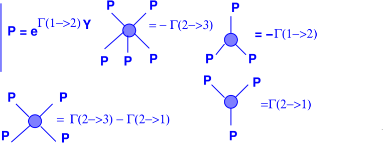
Figure 4: Pomeron interactions described by Eq. (6.52).

As we see from Fig. 4 two vertices $\Gamma(2\rightarrow 1)$ and $\Gamma(2\rightarrow 3)$ are responsible for different processes of Pomeron interaction. At first sight $\Gamma(2\rightarrow 1)$ is much smaller than $\Gamma(2\rightarrow 3)$ and can be neglected. However, we can make such a conclusions only if we will find out what value of $u$ ( or $\gamma$) are essential for high energies. Therefore, the vertex $\Gamma(2\rightarrow 1)$ can be still relevant in certain kinematic domains. To answer this question we need a detailed analysis of Eq. (2.4) and Eq. (4.38) which is beyond the scope of this paper (this question is addressed in Ref. [35]).

Fig. 5 presents some examples of Pomeron diagrams which correspond to different approaches that has been discussed in the past: the GLR equation [8] (see Fig. 5-a) which, in our approximation, coincides with the BK [5, 6] and JIMWLK [11] equations; the Iancu-Mueller approach [12] (see Fig. 5-b). Fig. 5-c shows a typical diagram that can be incorporated using Eq. (6.52). Finally, in Fig. 5-d we plot the diagrams that one needs to sum in order to reliably consider nucleus - nucleus interactions. In general such diagrams are difficult to sum, but we have an experience that in the simple model of Eq. (6.52), this summation can be performed [13, 36].

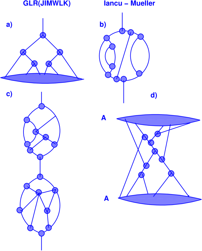
Figure 5: The typical Pomeron diagrams for interactions described by Eq. (6.52). Fig. 5-a describes the GLR approach [8] which for Eq. (6.52) coincide with the Balitsky-JIMWLK approach [11, 5]; Fig. 5-b corresponds to Iancu-Mueller approach[12] which suggests the way out of the JIMWLK approach and can be justified in limited region of energy. Fig. 5-c shows the general type of the diagrams that can be summed in the framework of the approach based on Eq. (6.52). Fig. 5-d are diagrams that we need to sum for nucleus-nucleus interaction at high energy.

It is important to stress that by introducing the vertex $\Gamma(2\,\rightarrow\,3)$, we have taken into account only the leading $N_{c}$ corrections. For $n$ dipole densities with $n>2$ we should have color correlations which cannot be presented in the dipole basis. We believe, however, that these correlations are of no significance at high energies.

The importance of correlations have been already noticed in Refs.[30, 31, 12]. Eq. (6.52) illustrates a complexity of the problem since even this oversimplified equation has not been solved. The expansion in correlations allows to shrink the infinite hierarchy of equations to a system of two coupled equations. This reduction provides a method for estimating importance of both the $N_{c}$ correlations and Pomeron loops. We demonstrated that correlations should be essential at high energies and suggested a consistent approach to take them into account.

In this paper we have considered a merging process of two Pomerons into one only. In general, there exist higher order processes accounting for a possibility of many Pomerons merging into one. A formal resummation of these processes has been reported in recent Ref. [37] and also in Ref. [41].

We hope that we propose the simplest way of dealing with the Pomeron loops which is equivalent to the reggeon calculus for BFKL Pomeron but has an advantage of clear probabilistic interpretation in the rest frame of one of the colliding particles. We hope that clarification of all assumptions in our approach will lead us to deeper and more transparent understanding of physics in the saturation domain.

Finally, let us comment on two recent papers [38, 28] which appeared practically simultaneously with ours and contain features close to those presented here. In fact the formal expression for the vertex $\Gamma(2\rightarrow 1)$ (Eq. (3.30)) is identical to the ones of Refs. [38, 28]. This equivalence has been proven in a later Ref. [39]. The main difference is that we have extended the method. Apart from giving the formal expression for the vertex $\Gamma(2\rightarrow 1)$, we also introduced a formalism needed for its evaluation (see Appendix). At the end, we were able to obtain a first analytical evaluation of the vertex bringing it to the level ready for computer simulations (Eq. (A.22)). The diagonal transition $2\rightarrow 2$, which guarantees probability conservation, vanishes if the exact expression for the vertex $\Gamma(2\rightarrow 1)$ is used. Generally this term should not be neglected if an approximate vertex is used for practical applications. In addition we have included the vertex $\Gamma(2\rightarrow 3)$ in our consideration.

Appendix A:   Calculation of $\Gamma\left(2\rightarrow 1\right)$.

In this appendix we find the solution to Eq. (3.28). Our approach is based on the main properties of the BFKL kernel which have been studies in details in Refs. [19, 20]. First, we rewrite Eq. (3.26) in the form of the contour integral over $h$ [19, 20], namely,

$$\gamma^{BA}\left(x,y;x^{\prime},y^{\prime}\right)\,\,=\,\,\frac{1}{2}\,\{\tilde{\gamma}_{BA}\left(x,y;x^{\prime},y^{\prime}\right)\,\,-\,\,\tilde{\gamma}_{BA}\left(x,y;y^{\prime},x^{\prime}\right)\}$$ (A.1)

where

$$\tilde{\gamma}_{BA}\left(x,y;x^{\prime},y^{\prime}\right)\,\,=$$ (A.2)

$$=\,\,\int^{a+i\infty}_{a-i\infty}\,\,\frac{d\,h}{2\,\pi\,i\,h^{3}}\,\tilde{\gamma}_{BA}\left(h;x,y;x^{\prime},y^{\prime}\right)\,\,=\,\,\frac{\bar{\alpha}_{S}^{2}}{16\,N^{2}_{c}}\,\int^{a+i\infty}_{a-i\infty}\,\,\frac{d\,h}{2\,\pi\,i}\,\frac{1}{h^{3}}\,\left(\frac{({x}-{y})^{2}\,({x}^{\,{}^{\prime}}-{y}^{\,{}^{\prime}})^{2}}{({x}-{x}^{\,{}^{\prime}})^{2}\,({y}-{y}^{\,{}^{\prime}})^{2}}\right)^{h}$$

where $x,y,x^{\prime}$ and $y^{\prime}$ is the coordinate of quarks and antiquarks in the interacting dipoles with the size $r=x-y$ and $r^{\prime}=x^{\prime}-y^{\prime}$. Introducing complex numbers instead of vectors $x=x_{1}+ix_{2}$ and $x^{*}=x_{1}-ix_{2}$ $(x\,x^{*}\,=\,({x})^{2})$, we can rewrite $\tilde{\gamma}_{BA}\left(h;x,y;x^{\prime},y^{\prime}\right)$ in the form:

$$\tilde{\gamma}_{BA}\left(h;x,y;x^{\prime},y^{\prime}\right)\,\,=\,\frac{\bar{\alpha}_{S}^{2}}{16\,N^{2}_{c}}\,\left(\frac{(x-y)\,(x^{\prime}-y^{\prime})}{(x-x^{\prime})\,(y-y^{\prime})}\right)^{h}\,\,\left(\frac{(x-y)^{*}\,(x^{\prime}-y^{\prime})^{*}}{(x-x^{\prime})^{*}\,(y-y^{\prime})^{*}}\right)^{h}\,\equiv\,\frac{\bar{\alpha}_{S}^{2}}{16\,N^{2}_{c}}\,\,\gamma_{BA}^{h}\,\times\,\gamma^{h\,*}_{BA}$$ (A.3)

At first sight Eq. (A.1) does not lead to Eq. (3.26). Indeed it gives

$$\gamma^{BA}\left(x,y;x^{\prime},y^{\prime}\right)\,\,=$$ (A.4)

$$=\,\,\frac{\bar{\alpha}_{S}^{2}}{32\,N^{2}_{c}}\,\ln\left(\frac{({x}-{y}^{\,{}^{\prime}})^{2}\,({y}-{x}^{\,{}^{\prime}})^{2}}{({x}-{x}^{\,{}^{\prime}})^{2}\,({y}-{y}^{\,{}^{\prime}})^{2}}\right)\,\,\,\ln\left(\frac{({x}-{y})^{4}\,({x}^{\,{}^{\prime}}-{y}^{\,{}^{\prime}})^{4}}{({y}-{x}^{\,{}^{\prime}})^{2}\,({x}-{y}^{\,{}^{\prime}})^{2}\,({y}-{y}^{\,{}^{\prime}})^{2}\,\,({x}-{x}^{\,{}^{\prime}})^{2}}\right)$$

The replacement of the Born amplitude Eq. (3.26) by Eq. (A.1) is a major step for what follows and has to be justified. We refer here to the work of Lipatov [19] who showed that the Born amplitude could be written in the form of Eq. (A.1) (see Eq.110 of the first paper in Ref. [19]). The main idea of Ref. [19] is that two expressions Eq. (A.1) and Eq. (3.26) lead to the very same results if used for calculations of physical observables (for example $\gamma-\gamma$ scattering). Both expressions satisfy Eq. (3.29) and hence they differ by a function $\xi$, which does not depend on one of the coordinates $x$ (or $y$). Lipatov showed that, thanks to the properties of the impact factor $\Phi(x,y,q)$ (see Eq. 109 in Ref. [19]), the integral over $x$ (or $y$) of the impact factor convoluted with $\xi$ vanishes. This property of the impact factor implies that a function, which does not depend on one of the coordinates, gives zero contribution to any physical process. Moreover, the well known BFKL Green function [21] was calculated using Eq. (A.1) as initial condition. To be consistent with the use of the BFKL kernel, Eq. (A.1) has to be taken as the Born approximation. We will see below that this replacement allows us to evaluate the vertex $\Gamma(2\rightarrow 1)$ (Eq. (3.30)).

In what follows we deal with the first term in Eq. (A.1) but it is a trivial algebraic exercise to obtain a result for the full Born amplitude of Eq. (A.1).

The r.h.s. of Eq. (3.28) we rewrite, using Eq. (A.2) and Eq. (A.3) in the form

$$\bar{\alpha}_{S}\,\int^{a+i\infty}_{a-i\infty}\,\,\frac{d\,h_{1}}{4\,\pi\,i}\,\frac{1}{h^{3}_{1}}\,\,\,\int^{a+i\infty}_{a-i\infty}\,\,\frac{d\,h_{2}}{4\,\pi\,i}\,\frac{1}{h^{3}_{2}}\,\int\,\,dz\,\,dz^{*}\,\left(\frac{x-y}{(x-z)\,(y-z)}\right)\,\cdot\,\left(\frac{x-y}{(x-z)\,(y-z)}\right)^{*}$$

$$\,\,\tilde{\gamma}_{BA}\left(h_{1};x,z;x_{1},y_{1}\right)\,\,\,\tilde{\gamma}_{BA}\left(h_{2};z,y;x_{2},y_{2}\right)$$ (A.5)

The integrals over $z$ and $z^{*}$ can be computed using formula 3.211, 9.182(1) and 9.183(1) of Ref. [40]. Indeed, Eq. (A.5) can be rewritten as follows

$$\frac{\bar{\alpha}_{S}^{3}}{(16\,N^{2}_{c})^{2}}\,\int^{a+i\infty}_{a-i\infty}\,\,\frac{d\,h_{1}}{4\,\pi\,i}\,\frac{1}{h^{3}_{1}}\,\,\,\int^{a+i\infty}_{a-i\infty}\,\,\frac{d\,h_{2}}{4\,\pi\,i}\,\frac{1}{h^{3}_{2}}\,\left(I\,\,I^{*}\right)$$ (A.6)

Using the notation $x-y=r$ and $x-z=r^{\prime}$, we have

$$I\,\,=\,\,\int\,dr^{\prime}\frac{r}{(r-r^{\prime})\,r^{\prime}}\,\left(\frac{r^{\prime}\,(x_{1}-y_{1})}{(x-x_{1})\,(x-r^{\prime}-y_{1})}\right)^{h_{1}}\left(\frac{(r^{\prime}-r)\,(x_{2}-y_{2})}{(y-y_{2})\,(x-r^{\prime}-x_{2})}\right)^{h_{2}}$$ (A.7)

We calculate $I$ dividing the integration over $r^{\prime}$ in three regions, namely,

$$I\,\,=\,\,I_{1}\left(-\infty\,<\,r^{\prime}\,<\,0\right)\,+\,I_{2}\left(0\,<r^{\prime}\,<\,r\right)\,+\,I_{3}\left(r\,<r^{\prime}\,<\,\infty\right)$$ (A.8)

Let us first compute the integral from the second region

$$I_{2}\,\, = \,\,\int_{0}^{r}\,dr^{\prime}\frac{r}{(r-r^{\prime})\,r^{\prime}}\,\left(\frac{r^{\prime}\,(x_{1}-y_{1})}{(x-x_{1})\,(x-r^{\prime}-y_{1})}\right)^{h_{1}}\left(\frac{(r^{\prime}-r)\,(x_{2}-y_{2})}{(y-y_{2})\,(x-r^{\prime}-x_{2})}\right)^{h_{2}}\,\,=$$

$$= \,\,\left(\frac{(x_{1}-y_{1})\,(x-y)}{(x-x_{1})\,(x-y_{1})}\right)^{h_{1}}\,\left(\frac{(x_{2}-y_{2})\,(x-y)}{(y-y_{2})\,(x-x_{2})}\right)^{h_{2}}\,\,$$

$$\times \,\,\frac{\Gamma(h_{1})\,\Gamma(h_{2})}{\Gamma(h_{1}+h_{2})}\,\,F_{1}\left(h_{1},h_{1},h_{2},h_{1}+h_{2},\frac{(x-y)}{(x-y_{1})},\frac{(x-y)}{(x-x_{2})}\right)$$

$$= \left(\frac{(x_{1}-y_{1})(x-y)}{(x-x_{1})\,(y-y_{1})}\right)^{h_{1}}\,\left(\frac{(x_{2}-y_{2})(x-y)}{(x-x_{2})\,(y-y_{2})}\right)^{h_{2}}\,\,$$

$$\times \frac{\Gamma(h_{1})\,\Gamma(h_{2})}{\Gamma(h_{1}+h_{2})}\,{}_{2}F_{1}\left(h_{1},h_{2},h_{1}+h_{2},\frac{(x-y)\,(x_{2}-y_{1})}{(x-x_{2})(y-y_{1})}\right)$$

$$\rightarrow \frac{(h_{1}+h_{2})}{h_{1}\,h_{2}}\,\left(\frac{(x_{1}-y_{1})(x-y)}{(x-x_{1})\,(y-y_{1})}\right)^{h_{1}}\,\left(\frac{(x_{2}-y_{2})(x-y)}{(x-x_{2})\,(y-y_{2})}\right)^{h_{2}}$$ (A.11)

Eq. (Appendix A:   Calculation of $\Gamma\left(2\rightarrow 1\right)$.) was obtained using 3.211 of Ref. [40]. Obtaining Eq. (A.11) we take into account that only small values of $h_{1}$ and $h_{2}$ will contribute to the integral of Eq. (A.5).

In Eq. (Appendix A:   Calculation of $\Gamma\left(2\rightarrow 1\right)$.) and Eq. (A.11) $F_{1}$ and ${}_{2}F_{1}\equiv F$ denote the hypergeometric functions (see formula 9.10 and 9.180(1) in Ref. [40]).

$I_{3}$ is the integral of Eq. (A.7) for $r^{\prime}>r$, namely,

$$I_{3}\,\, = \,\,\int_{r}\,dr^{\prime}\frac{r}{(r-r^{\prime})\,r^{\prime}}\,\left(\frac{r^{\prime}\,(x_{1}-y_{1})}{(x-x_{1})\,(x-r^{\prime}-y_{1})}\right)^{h_{1}}\left(\frac{(r-r^{\prime})\,(x_{2}-y_{2})}{(y-y_{2})\,(x-r^{\prime}-x_{2})}\right)^{h_{2}}\,=$$

$$= \,\,\left(\frac{(x_{1}-y_{1})}{(x-x_{1})}\right)^{h_{1}}\,\left(\frac{(x_{2}-y_{2})}{(y-y_{2})}\right)^{h_{2}}\,\,$$

$$\times \,\,\frac{\Gamma(1)\,\Gamma(h_{2})}{\Gamma(1+h_{2})}\,\,F_{1}\left(1,h_{1},h_{2},1+h_{2},\frac{(y-y_{1})}{(x-y)},\frac{(y-y_{2})}{(x-y)}\right)$$

$$\rightarrow \,\,\frac{1}{h_{2}}\left(\frac{(x_{1}-y_{1})}{(x-x_{1})}\right)^{h_{1}}\,\left(\frac{(x_{2}-y_{2})}{(y-y_{2})}\right)^{h_{2}}$$ (A.13)

In Eq. (A.13) we found the limit at small values of $h_{2}$ which contribute to the integral of Eq. (A.5). The third integral is equal to

$$I_{1}\,\, = \,\,\int_{-\infty}^{0}\,dr^{\prime}\frac{r}{(r-r^{\prime})\,r^{\prime}}\,\left(\frac{r^{\prime}\,(x_{1}-y_{1})}{(x-x_{1})\,(x-r^{\prime}-y_{1})}\right)^{h_{1}}\left(\frac{(r-r^{\prime})\,(x_{2}-y_{2})}{(y-y_{2})\,(x-r^{\prime}-x_{2})}\right)^{h_{2}}\,=$$ (A.14)

$$\rightarrow \,\,\frac{1}{h_{1}}\left(\frac{(x_{1}-y_{1})}{(x-x_{1})}\right)^{h_{1}}\,\left(\frac{(x_{2}-y_{2})}{(y-y_{2})}\right)^{h_{2}}$$

Substituting Eq. (A.11) and Eq. (A.13) into Eq. (A.6) we finally obtain the result for the r.h.s. of Eq. (3.28), namely,

$$\frac{\bar{\alpha}_{S}^{5}}{(16\,N^{2}_{c})^{2}}\,\int^{a+i\infty}_{a-i\infty}\,\,\frac{d\,h_{1}}{4\,\pi\,i}\,\frac{1}{h^{3}_{1}}\,\,\,\int^{a+i\infty}_{a-i\infty}\,\,\frac{d\,h_{2}}{4\,\pi\,i}\,\frac{1}{h^{3}_{2}}\,\left(\frac{(h_{1}+h_{2})}{h_{1}\,h_{2}}\right)^{2}\,\times$$ (A.15)

$$\left(\left(\frac{(x_{1}-y_{1})(x-y)}{(x-x_{1})\,(y-y_{1})}\right)^{h_{1}}\,\left(\frac{(x_{2}-y_{2})(x-y)}{(x-x_{2})\,(y-y_{2})}\right)^{h_{2}}\,+\,\left(\frac{({x}_{1}-{y}_{1})}{({x}-{x}_{1})}\right)^{h_{1}}\,\left(\frac{({x}_{2}-{y}_{2})}{({y}-{y}_{2})}\right)^{h_{2}}\right)\,\times$$

$$\left(\left(\frac{(x_{1}-y_{1})(x-y)}{(x-x_{1})\,(y-y_{1})}\right)^{h_{1}}\,\left(\frac{(x_{2}-y_{2})(x-y)}{(x-x_{2})\,(y-y_{2})}\right)^{h_{2}}\,+\,\left(\frac{({x}_{1}-{y}_{1})}{({x}-{x}_{1})}\right)^{h_{1}}\,\left(\frac{({x}_{2}-{y}_{2})}{({y}-{y}_{2})}\right)^{h_{2}}\,\right)^{*}$$

The integrals over $h_{1}$ and $h_{2}$ can be evaluated but we postpone this until we work out the action of Laplacians (Eq. (3.30)).

As was noticed in Section 3, the Born amplitude in the form of Eq. (A.2) as well as of Eq. (3.26) satisfy the following equation

$$\Delta_{x}\,\Delta_{y}\,\tilde{\gamma}_{BA}\left(x,y;x^{\prime},y^{\prime}\right)\,\,\equiv\,\frac{d}{dx}\,\frac{d}{dx^{*}}\,\frac{d}{dy}\,\frac{d}{dy^{*}}\,\tilde{\gamma}_{BA}\left(x,y;x^{\prime},y^{\prime}\right)\,\,\,$$ (A.16)

$$=\,\,\alpha_{S}^{2}\left(\delta^{(2)}\left({x}-{x}^{\,{}^{\prime}}\right)\delta^{(2)}\left({y}-{y}^{\,{}^{\prime}}\right)\,+\,\delta^{(2)}\left({x}-{y}^{\,{}^{\prime}}\right)\delta^{(2)}\left({y}-{x}^{\,{}^{\prime}}\right)\right)$$

Thus $\Gamma(2\rightarrow 1)$ (see Eq. (3.30)) is obtained by applying operator $\Delta_{x}\,\Delta_{y}$ to Eq. (A.15) and multiplying by $N_{c}^{2}/\bar{\alpha}_{s}^{2}$. The observation which helps to simplify the calculation is the following:

$$\frac{d}{dx}\,\frac{d}{dy}\,I_{2}\,\,=\,\,\left(\frac{1}{h_{1}}+\frac{1}{h_{2}}\right)\,\left(\left(h_{1}\,+\,h_{2}\right)\,\frac{1}{(x-y)^{2}}\,\,\,+\,\,O(h^{2})\right)\,I_{2}\,,$$ (A.17)

where we can neglect terms that are proportional to $h_{1}^{2}$ or $h^{2}_{2}$, as the dominant contribution to Eq. (A.16) stems from the region of small $h$’s. Similarly the contribution originating from the integrals $I_{1}$ and $I_{3}$ can be neglected since

$$\frac{d}{dx}\,\frac{d}{dy}\,I_{1}\,\,\propto\,\,h^{2}_{1}\frac{1}{h_{1}}\,$$ (A.18)

Taking into account Eq. (A.17) and Eq. (A.18) we obtain

$$\Gamma_{2\rightarrow 1}\left((x_{1},y_{1})+(x_{2},y_{2})\,\rightarrow\,(x,y)\right)\,\,=\,\,\frac{N_{c}}{\pi\,\alpha_{s}}\,\int^{a+i\infty}_{a-i\infty}\,\,\frac{d\,h_{1}}{4\,\pi\,i}\,\frac{1}{h^{3}_{1}}\,\,\,\int^{a+i\infty}_{a-i\infty}\,\,\frac{d\,h_{2}}{4\,\pi\,i}\,\frac{1}{h^{3}_{2}}\,\,\frac{(h_{1}+h_{2})^{4}}{h^{2}_{1}\,h^{2}_{2}}$$ (A.19)

$$\frac{1}{({x}-{y})^{4}}\,\,\tilde{\gamma}_{BA}\left(h_{1};x,y;x_{1},y_{1}\right)\,\,\tilde{\gamma}_{BA}\left(h_{2};x,y;x_{2},y_{2}\right)\$$

Now we can easily evaluate the remaining integrals over $h_{1}$ and $h_{2}$. The result can be written in the most economic form introducing a new variable:

$$R\left(x,y;x^{\prime},y^{\prime}\right)\,\,=\,\,\frac{({x}-{y})^{2}\,\,({x}^{\,\,{}^{\prime}}-{y}^{\,\,{}^{\prime}})^{2}}{({x}-{x}^{\,\,{}^{\prime}})^{2}\,\,({y}-{y}^{\,\,{}^{\prime}})^{2}}$$ (A.20)

The vertex reads

$$\Gamma_{2\rightarrow 1}\left((x_{1},y_{1})+(x_{2},y_{2})\,\rightarrow\,(x,y)\right)\,\,=\,\,\frac{\bar{\alpha}_{S}^{3}}{(32\,\pi)^{2}\,\,N^{2}_{c}}\,\,\frac{1}{({x}-{y})^{4}}\,\,\left(\frac{1}{24}\,\ln^{4}R\left(x,y;x_{1},y_{1}\right)\,+\right.$$ (A.21)

$$\left.\,\frac{2}{3}\,\ln^{3}R\left(x,y;x_{1},y_{1}\right)\ln R\left(x,y;x_{2},y_{2}\right)\,+\,\frac{3}{2}\,\ln^{2}R\left(x,y;x_{1},y_{1}\right)\ln^{2}R\left(x,y;x_{2},y_{2}\right)\,+\right.$$

$$\left.\,\,+\,\,\frac{2}{3}\,\ln R\left(x,y;x_{1},y_{1}\right)\ln^{3}R\left(x,y;x_{2},y_{2}\right)\,+\,\frac{1}{24}\,\ln^{4}R\left(x,y;x_{2},y_{2}\right)\right)$$

So far, we evaluated the contribution of the first term ($\gamma_{BA}^{(1)}$) of the full Born amplitude of Eq. (A.1). Having added the second term we end up with the final expression for the vertex:

$$\Gamma_{2\rightarrow 1}\left((x_{1},y_{1})+(x_{2},y_{2})\,\rightarrow\,(x,y)\right)\,=\,\frac{\bar{\alpha}_{S}^{3}}{2\,(32\,\pi)^{2}\,N^{2}_{c}}\,\,\frac{1}{({x}-{y})^{4}}\,\ln\frac{R\left(x,y;x_{1},y_{1}\right)}{R\left(x,y;y_{1},x_{1}\right)}\,\ln\frac{R\left(x,y;x_{2},y_{2}\right)}{R\left(x,y;y_{2},x_{2}\right)}\times$$

$$\left(\,\frac{2}{3}\,[\ln^{2}R\left(x,y;x_{1},y_{1}\right)\,\,+\,\,\ln R\left(x,y;x_{1},y_{1}\right)\,\ln R\left(x,y;y_{1},x_{1}\right)\,\,+\,\,\ln^{2}R\left(x,y;y_{1},x_{1}\right)]\,\,+\right.$$

$$\left.\,+\,\frac{3}{2}\,\ln(R\left(x,y;x_{1},y_{1}\right)\,R\left(x,y;y_{1},x_{1}\right))\,\ln(R\left(x,y;x_{2},y_{2}\right)R\left(x,y;y_{2},x_{2}\right))\,+\right.$$ (A.22)

$$\left.\,\,+\,\,\frac{2}{3}\,[\ln^{2}R\left(x,y;x_{2},y_{2}\right)\,\,+\,\,\ln R\left(x,y;x_{2},y_{2}\right)\,\ln R\left(x,y;y_{2},x_{2}\right)\,\,+\,\,\ln^{2}R\left(x,y;y_{2},x_{2}\right)]\right)$$

References

- [1] A. H. Mueller, Nucl. Phys. B 415 (1994) 373; ibid B 437 (1995) 107.
- [2] E. Levin and M. Lublinsky, Nucl. Phys. A730 (2004) 191 [arXiv:hep-ph/0308279].
- [3] E. Levin and M. Lublinsky, Phys. Lett. B 607 (2005) 131.
- [4] R. A. Janik, “B-JIMWLK in the dipole sector,” arXiv:hep-ph/0409256; R. A. Janik and R. Peschanski, Phys. Rev. D70 (2004) 094005 [arXiv:hep-ph/0407007].
- [5] I. Balitsky, Nucl. Phys. B463 (1996) 99 [arXiv:hep-ph/9509348].
- [6] Y. V. Kovchegov, Phys. Rev. D60 (1999) 034008 [arXiv:hep-ph/9901281].
-
[7]
M. Lublinsky,
Eur. Phys. J. C 21 (2001) 513;
E. Levin and M. Lublinsky,
Nucl. Phys. A 712 (2002) 95.
N. Armesto and M. Braun, Eur. Phys. J. C 20 (2001) 517;
K. Golec-Biernat, L. Motyka, A. Stasto, Phys. Rev. D 65 (2002) 074037;
E. Gotsman, E. Levin, M. Lublinsky and U. Maor, Eur. Phys. J C 27 (2003) 411;
E. Gotsman, E. Levin, M. Lublinsky, U. Maor and E. Naftali, Acta Phys. Polon. B 34, 3255 (2003); G. Chachamis, M. Lublinsky and A. Sabio-Vera, Nucl. Phys. A 748, 649 (2005); K. Kutak and A.M. Stasto, hep-ph/0408117;
J. Albacete et.al., Phys. Rev. Lett. 92 (2004) 082001. - [8] L. V. Gribov, E. M. Levin and M. G. Ryskin, Phys. Rep. 100 (1983) 1.
- [9] A. H. Mueller and J. Qiu, Nucl. Phys. B 268 (1986) 427.
- [10] L. McLerran and R. Venugopalan, Phys. Rev. D 49 (1994) 2233, 3352; D 50 (1994) 2225, D 53 (1996) 458, D 59 (1999) 09400.
-
[11]
J. Jalilian Marian, A. Kovner, A.Leonidov and H.
Weigert,
Nucl. Phys. B504 (1997) 415; Phys. Rev. D59 (1999) 014014; J. Jalilian Marian, A. Kovner and H. Weigert, Phys. Rev. D59 (1999) 014015;
A. Kovner and J.G. Milhano, Phys. Rev. D61 (2000) 014012.
A. Kovner, J.G. Milhano and H. Weigert,
Phys. Rev. D62:114005,2000; H. Weigert, Nucl. Phys. A703 (2002) 823;
E. Iancu, A. Leonidov and L. D. McLerran, Phys. Lett. B510 (2001) 133 [arXiv:hep-ph/0102009]; Nucl. Phys. A692 (2001) 583 [arXiv:hep-ph/0011241];
H. Weigert, Nucl. Phys. A703 (2002) 823 [arXiv:hep-ph/0004044]. - [12] E. Iancu and A. H. Mueller, Nucl. Phys. A730 (2004) 460, 494, [arXiv:hep-ph/0308315],[arXiv:hep-ph/0309276].
- [13] M. Braun, Phys. Lett. B 483 (2000) 115.
- [14] J. Bartels, Z. Phys. C 60, 471 (1993); J. Bartels and M. Wusthoff, Z. Phys. C 66, 157 (1995).
- [15] M. Kozlov and E. Levin, Nucl. Phys. A739 (2004) 291 [arXiv:hep-ph/0401118].
- [16] A. H. Mueller and A. I. Shoshi, Nucl. Phys. B 692 (2004) 175 [arXiv:hep-ph/0402193].
- [17] E. Iancu, A. H. Mueller and S. Munier, Phys. Lett. B 606 (2005) 342.
- [18] I. Balitsky, Phys. Rev. D 70 (2004) 114030.
- [19] L. N. Lipatov, Phys. Rept. 286, 131 (1997) [arXiv:hep-ph/9610276]; Sov. Phys. JETP 63 (1986) 904.
- [20] H. Navelet and R. Peschanski, Nucl. Phys. B634 (2002) 291 [arXiv:hep-ph/0201285]; Phys. Rev. Lett. 82 (1999) 137,, [arXiv:hep-ph/9809474]; Nucl. Phys. B507 (1997) 353, [arXiv:hep-ph/9703238] A. Bialas, H. Navelet and R. Peschanski, Phys. Rev. D57 (1998) 6585; R. Peschanski, Phys. Lett. B409 (1997) 491.
-
[21]
E. A. Kuraev, L. N. Lipatov, and F. S. Fadin, Sov. Phys. JETP
45 (1977) 199 ;
Ya. Ya. Balitsky and L. N. Lipatov, Sov. J. Nucl. Phys. 28 (1978) 22 . - [22] P. Grassberger and K. Sundermeyer, Phys. Lett. B77 (1978) 220.
- [23] E. Levin, Phys. Rev. D 49 (1994) 4469.
- [24] K. G. Boreskov, “Probabilistic model of Reggeon field theory,” arXiv:hep-ph/0112325.
- [25] J. Bartels, Nucl. Phys. B175, 365 (1980); J. Kwiecinski and M. Praszalowicz, Phys. Lett. B94, 413 (1980).
-
[26]
V. N. Gribov and L. N. Lipatov, Sov. J. Nucl. Phys 15 (1972)
438;
G. Altarelli and G. Parisi, Nucl. Phys. B 126 (1977) 298;
Yu. l. Dokshitser, Sov. Phys. JETP 46 (1977) 641. - [27] E. Iancu and D. N. Triantafyllopoulos, Nucl. Phys. A 756 (2005) 419.
- [28] E. Iancu and D.N. Triantafyllopoulos, Phys. Lett. B 610 253 (2005).
- [29] I. F. Ginzburg, S.L. Panfil and V.G. Serbo, Nucl. Phys. B284 (1987) 685, B296 (1988) 569; I. F. Ginzburg and D. Yu. Ivanov, Nucl. Phys. B388 (1992) 376; D. Y. Ivanov and R. Kirschner, Phys. Rev. D58 (1998) 114026, hep-ph/9807324; M. Kozlov and E. Levin, Eur. Phys. J. C 28 (2003) 483 [arXiv:hep-ph/0211348].
- [30] J. Bartels, Phys. Lett. B298 (1993) 204; E. M. Levin, M. G. Ryskin and A. G. Shuvaev,Nucl. Phys. B387 (1992) 589.
- [31] E. Laenen and E. Levin, Nucl. Phys. B 451 (1995) 207 [arXiv:hep-ph/9503381]; Ann. Rev. Nucl. Part. Sci. 44 (1994) 199; E. Laenen, E. Levin and A. G. Shuvaev, Nucl. Phys. B 419 (1994) 39 [arXiv:hep-ph/9308294].
- [32] Z. Chen and A. H. Mueller, Nucl. Phys. B 451, 579 (1995).
- [33] A Kovner and M. Lublinsky, JHEP 0503, 001 (2005).
- [34] J. Bartels, L. N. Lipatov and G. P. Vacca, Phys. Lett. B 477 (2000) 178 [arXiv:hep-ph/9912423].
- [35] E. Levin, arXiv:hep-ph/0502243.
-
[36]
D. Amati, L. Caneschi and R. Jengo,
Nucl. Phys. B 101 (1975) 397.
A. Schwimmer, Nucl. Phys. B 94 (1975) 445;
S. Bondarenko, E. Gotsman, E. Levin and U. Maor, Nucl. Phys. A683 (2001) 649 [arXiv:hep-ph/0001260]. - [37] A. Kovner and M. Lublinsky, Phys. Rev. D 71 (2005) 085004; Phys. Rev. Lett. 94, 181603 (2005).
- [38] A. H. Mueller, A. I. Shoshi and S. M. H. Wong, Nucl. Phys. B 715, 440 (2005)
- [39] A. Kovner and M. Lublinsky, arXiv:hep-ph/0503155.
- [40] I. Gradstein and I. Ryzhik, “ Tables of Series, Products, and Integrals”, Verlag MIR, Moskau,1981.
- [41] Y. Hatta, E. Iancu, L. McLerran, A. Stasto and D. N. Triantafyllopoulos, arXiv:hep-ph/0504182.