Higgs boson production at hadron colliders
in the $k_{T}$-factorization approach

D.V. Skobeltsyn Institute of Nuclear Physics,
M.V. Lomonosov Moscow State University,
119992 Moscow, Russia

Abstract

We consider the Higgs boson production at high energy hadron colliders in the framework of the $k_{T}$-factorization approach. The attention is focused on the dominant gluon-gluon fusion subprocess. We calculate the total cross section and transverse momentum distributions of the inclusive Higgs production using unintegrated gluon distributions in a proton obtained from the full CCFM evolution equation. We show that $k_{T}$-factorization gives a possibility to investigate the associated Higgs boson and jets production. We calculate the transverse momentum distributions and study the Higgs-jet and jet-jet azimuthal correlations in the Higgs + one or two jet production processes. We demonstrate the importance of the higher-order corrections within the $k_{T}$-factorization approach. These corrections should be developed and taken into account in the future applications.

1 Introduction

It is well known that the electroweak symmetry breaking in the Standard Model of elementary particle interactions is achieved via the Higgs mechanism. In the minimal model there are a single complex Higgs doublet, where the Higgs boson $H$ is the physical neutral Higgs scalar which is the only remaining part of this doublet after spontaneous symmetry breaking. In non-minimal models there are additional charged and neutral scalar Higgs particles. The search for the Higgs boson takes important part at the Fermilab Tevatron experiments and will be one of the main fields of study at the CERN LHC collider [1]. The experimental detection of the $H$ will be great triumph of the Standard Model of electroweak interactions and will mark new stage in high energy physics.

At LHC conditions, the gluon-gluon fusion $gg\to H$ is the dominant inclusive Higgs production mechanism [2, 3]. In this process, the Higgs production occurs via triangle heavy (top) quark loop. The gluon fusion and weak boson fusion ($qq\to qqH$ subprocess via $t$-channel exchange of a $W$ or $Z$ bosons) are also expected to be the dominant sources of semi-inclusive Higgs production (in association with one or two hadronic jets) [4]. The detailed theoretical studies of such processes are necessary, in particular, to determine an optimal set of cuts on the final state particles.

It is obvious that the gluon-gluon fusion contribution to the Higgs production at LHC is strongly dependend on the gluon density $xG(x,\mu^{2})$ in a proton. Usually gluon density are described by the Dokshitzer-Gribov-Lipatov-Altarelli-Parizi (DGLAP) evolution equation [5] where large logarithmic terms proportional to $\ln\mu^{2}$ are taken into account. The cross sections can be rewritten in terms of hard matrix elements convoluted with gluon density functions. In this way the dominant contributions come from diagrams where the parton emissions in the initial state are strongly ordered in virtuality. This is called collinear factorization, as the strong ordering means that the virtuality of the parton entering the hard scattering matrix elements can be neglected compared to the large scale $\mu^{2}$. However, at the LHC energies, typical values of the incident gluon momentum fractions $x\sim m_{H}/\sqrt{s}\sim 0.008$ (for Higgs boson mass $m_{H}=120$ GeV) are small, and another large logarithmic terms proportional to $\ln 1/x$ become important. These contributions can be taken into account using Balitsky-Fadin-Kuraev-Lipatov (BFKL) evolution equation [6]. Just as for DGLAP, in this way it is possible to factorize an observable into a convolution of process-dependent hard matrix elements with universal gluon distributions. But as the virtualities (and transverse momenta) of the propagating gluons are no longer ordered, the matrix elements have to be taken off-shell and the convolution made also over transverse momentum ${\mathbf{k}}_{T}$ with the unintegrated ($k_{T}$-dependent) gluon distribution ${\cal F}(x,{\mathbf{k}}_{T}^{2})$. The unintegrated gluon distribution ${\cal F}(x,{\mathbf{k}}_{T}^{2})$ determines the probability to find a gluon carrying the longitudinal momentum fraction $x$ and the transverse momentum ${\mathbf{k}}_{T}$. This generalized factorization is called $k_{T}$-factorization [7–10]. It is expected that BFKL evolution gives the theoretically correct description at assymptotically large energies (i.e. very small $x$). At the same time another approach, valid for both small and large $x$, have been developed by Ciafaloni, Catani, Fiorani and Marchesini, and is known as the CCFM model [11]. It introduces angular ordering of emissions to correctly treat gluon coherence effects. In the limit of asymptotic energies it is almost equivalent to BFKL [12–14], but also similar to the DGLAP evolution for large $x$ and high $\mu^{2}$. The resulting unintegrated gluon distribution depends on two scales, the additional scale ${\bar{q}}^{2}$ is a variable related to the maximum angle allowed in the emission and plays the role of the evolution scale $\mu^{2}$ in the collinear parton densities. The following classification scheme [15] is used: ${\cal F}(x,{\mathbf{k}}_{T}^{2})$ denote pure BFKL-type unintegrated gluon distributions and ${\cal A}(x,{\mathbf{k}}_{T}^{2},\mu^{2})$ stands for any other type having two scale involved. In this paper we will apply the CCFM gluon evolution to study of the inclusive and semi-inclusive Higgs production at LHC conditions.

In the collinear factorization, the calculation of such processes is quite complicated even at lowest order because of the heavy quark loops contribution. For example, in Higgs + one jet production, triangle and box loops occur, and in Higgs + two jet production the pentagon loops occur [16]. However, the calculations of the Higgs production rates can be simplified in the limit of large top quark mass $m_{t}\to\infty$ [17]. In this approximation the coupling of the gluons to the Higgs via top-quark loop can be replaced by an effective coupling. Thus it reduces the number of loops in a given diagram by one. The large $m_{t}$ approximation is valid to an accuracy of $\sim 5$% in the intermediate Higgs mass range $m_{H}<2m_{t}$, as long as transverse momenta of the Higgs or final jets are smaller than of the top quark mass ($p_{T}<m_{t}$) [16]. Within this approach, the total cross section for $gg\to H+X$ is known to next-to-next-to-leading order (NNLO) accuracy [18]. Higher-order QCD corrections to inclusive Higgs production were found to be large: their effect increases the leading order cross section by about $80-100$% [19] (see also [20]).

A particularly interesting quantity is the transverse momentum distribution of the produced Higgs boson. The precise theoretical prediction of the $d\sigma/dp_{T}$ at the LHC is important for quantitative evaluation of the required measurement accuracies and detector performance. It is well-known that the fixed-order perturbative QCD is applicable when the Higgs transverse momentum is comparable to the $m_{H}$. Hovewer, the main part of the events is expected in the small-$p_{T}$ region ($p_{T}\ll m_{H}$), where the coefficients of the perturbative series in $\alpha_{s}$ are enhanced by powers of large logarithmic terms proportional to $\ln m_{H}^{2}/p_{T}^{2}$. Therefore reliable predictions at small $p_{T}$ can only be obtained if these terms will be resummed to all orders. Such procedure is called soft-gluon resummation [21-23] and has been performed in collinear calculations at leading logarithmic (LL), next-to-leading logarithmic (NLL) [24] and next-to-next-to-leading logarithmic (NNLL) [25] levels. Recently it was shown [26] that in the framework of $k_{T}$-factorization approach the soft gluon resummation formulas are the result of the approximate treatment of the solutions of the CCFM evolution equation (in the $b$-representation).

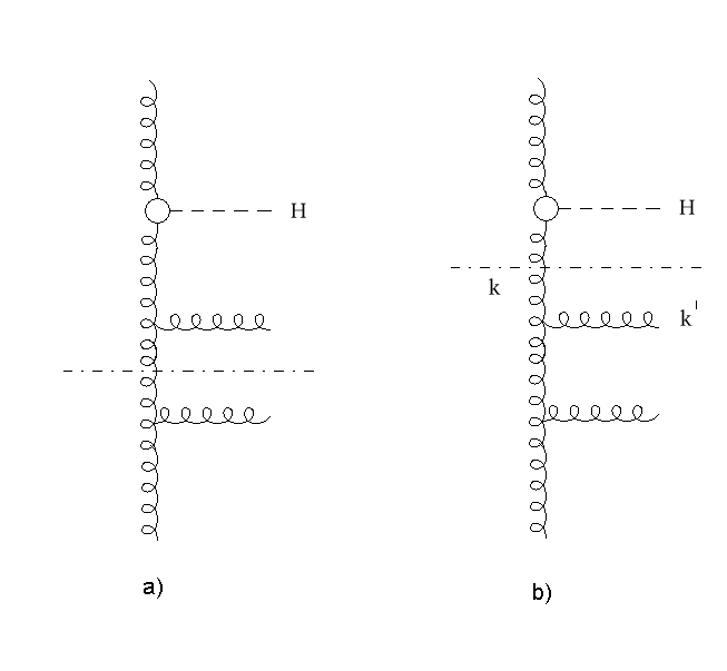
Figure 1: The typical Feynman diagram contributing to the Higgs boson production in the collinear (a) and $k_{T}$-factorization (b) approaches.

There are several additional motivations for our study of the Higgs production in the $k_{T}$-factorization approach. First of all, in the standard collinear approach, when the transverse momentum of the initial gluons is neglected, the transerse momentum of the final Higgs boson in $gg\to H$ subprocess is zero. Therefore it is necessary to include an initial-state QCD radiation to generate the $p_{T}$ distributions. It is well known at present that the $k_{T}$-factorization naturally includes a large part of the high-order perturbative QCD corrections [27]. This fact is illustrated more detailed in Figure 1, which is a schematical representation of a typical Higgs + jet production process. Figure 1 (a) shows the fixed-order perturbative QCD picture where the upper part of the diagram (above the dash-dotted line) corresponds to the $gg\to gH$ subrocess, and the lower part describes the gluon evolution in a proton. As the incoming gluons are assumed to have zero transverse momentum, the transverse momentum distributions of the produced Higgs and jet are totally determined by the properties of the ${\cal O}(\alpha_{s}^{3})$ matrix element. In the $k_{T}$-factorization approach (Figure 1 (b)), the underlying partonic subprocess is $gg\to H$, which is formally of order ${\cal O}(\alpha_{s}^{2})$. Some extra powers of $\alpha_{s}$ are hidden in the gluon evolution represented by the part of the diagram shown below the dash-dotted line. In contrast with the collinear approximation, the $k_{T}$-factorization takes into account the gluon transverse motion. Since the upper gluon in the parton ladder is not included in the hard interaction, its transverse momentum is now determined by the properties of the evolution equation only. It means that in the $k_{T}$-factorization approach the study of transverse momenta distributions in the Higgs production via gluon-gluon fusion will be direct probe of the unintegrated gluon distributions in a proton. In this case the transverse momentum of the produced Higgs should be equal to the sum of the transverse momenta of the initial gluons. Therefore future experimental studies at LHC can be used as further test of the non-collinear parton evolution.

In the previous studies [26, 28, 29] the $k_{T}$-factorization formalism was applied to calculate transverse momentum distribution of the inclusive Higgs production. The simplified solution of the CCFM equation in single loop approximation [30] (when small-$x$ effects can be neglected) were used in  [26]. In such approximation the CCFM evolution is reduced to the DGLAP one with the difference that the single loop evolution takes the gluon transverse momentum $k_{T}$ into account. Another simplified solution of the CCFM equation was proposed in Ref. [31], where the transverse momenta of the incoming gluons are generated in the last evolution step (Kimber-Martin-Ryskin prescription). The calculations [26, 29] were done using the on-mass shell (independent from the gluon $k_{T}$) matrix element of the $gg\to H$ subprocess and rather the similar results have been obtained. In Ref. [28] in the framework of MC generator CASCADE [32] the off-mass-shell matrix element obtained by F. Hautmann [33] has been used with full CCFM evolution.

In present paper we investigate Higgs production at hadron colliders using the full CCFM-evolved unintegrated gluon densities [28]. We obtain the obvious expression for the $g^{*}g^{*}\to H$ off-mass-shell matrix element in the large $m_{t}$ limit apart from Ref. [33]. After that, we calculate the total cross section and transverse momentum distribution of the inclusive Higgs production at Tevatron and LHC. To illustrate the fact that in the $k_{T}$-factorization approach the main features of collinear higher-order pQCD corrections are taken into account effectively, we give theoretical predictions for the Higgs + one jet and Higgs + two jet production processes using some physically motivated approximation.

In Section 2 we recall the basic formulas of the $k_{T}$-factorization formalism with a brief review of calculation steps. In Section 3 we present the numerical results of our calculations and discussion. Finally, in Section 4, we give summary of our results.

2 Basic formulas

We start from the effective Lagrangian for the Higgs boson coupling to gluons [16]:

$${\cal L}_{\rm{eff}}={\alpha_{s}\over 12\pi}\left(G_{F}\sqrt{2}\right)^{1/2}G_{\mu\nu}^{a}G^{a\,\mu\nu}H,$$

where $G_{F}$ is the Fermi coupling constant, $G_{\mu\nu}^{a}$ is the gluon field strength tensor and $H$ is the Higgs field. The triangle vertex $T^{\mu\nu}(k_{1},k_{2})$ for two off-shell gluons having four-momenta $k_{1}$ and $k_{2}$ and color indexes $a$ and $b$ respectively, can be obtained easily from the Lagrangian (1):

$$T^{\mu\nu}(k_{1},k_{2})=i\delta^{ab}{\alpha_{s}\over 3\pi}\left(G_{F}\sqrt{2}\right)^{1/2}\left[k_{2}^{\mu}k_{1}^{\nu}-(k_{1}\cdot k_{2})g^{\mu\nu}\right].$$

To calculate the squared off-mass-shell matrix element for the $g^{*}g^{*}\to H$ subprocess it is necessary to take into account the non-zero virtualities of the initial gluons $k_{1}^{2}=-{\mathbf{k}}_{1T}^{2}\neq 0$, $k_{2}^{2}=-{\mathbf{k}}_{2T}^{2}\neq 0$. We have obtained

$$|\bar{\cal M}|^{2}(g^{*}g^{*}\to H)={\alpha_{s}^{2}(\mu^{2})\over 576\pi^{2}}G_{F}\sqrt{2}\left[m_{H}^{2}+{\mathbf{k}}_{1T}^{2}+{\mathbf{k}}_{2T}^{2}+2|{\mathbf{k}}_{1T}||{\mathbf{k}}_{2T}|\cos\phi\right]^{2}\cos^{2}\phi,$$

where $\phi$ is the azimuthal angle between transverse momenta ${\mathbf{k}}_{1T}$ and ${\mathbf{k}}_{2T}$, the transverse momentum of the produced Higgs boson is ${\mathbf{p}}_{T}={\mathbf{k}}_{1T}+{\mathbf{k}}_{2T}$ and the virtual gluon polarization tensor has been taken in the form [7, 8]

$$\sum\epsilon^{\mu}\epsilon^{*\,\nu}={k_{T}^{\mu}k_{T}^{\nu}\over{\mathbf{k}}_{T}^{2}}.$$

The cross section of the inclusive Higgs production $p\bar{p}\to H+X$ in the $k_{T}$-factorization approach can be written as

$$d\sigma(p\bar{p}\to H+X)=\int{dx_{1}\over x_{1}}{\cal A}(x_{1},{\mathbf{k}}_{1T}^{2},\mu^{2})d{\mathbf{k}}_{1T}^{2}{d\phi_{1}\over 2\pi}\times\atop\displaystyle\times\int{dx_{2}\over x_{2}}{\cal A}(x_{2},{\mathbf{k}}_{2T}^{2},\mu^{2})d{\mathbf{k}}_{2T}^{2}{d\phi_{2}\over 2\pi}d\hat{\sigma}(g^{*}g^{*}\to H),$$

where $\hat{\sigma}(g^{*}g^{*}\to H)$ is the Higgs production cross section with off-mass-shell gluons, $x_{1}$ and $x_{2}$ are the longitudinal momentum fractions, and ${\cal A}(x,{\mathbf{k}}_{T}^{2},\mu^{2})$ is the unintegrated gluon distributions in a proton. Let $s=(p_{1}+p_{2})^{2}$ and $p_{1}$, $p_{2}$ are the four-vectors of the incoming protons. Then the differential cross section reads

$${d\sigma(p\bar{p}\to H+X)\over dy_{H}}=\int{\alpha_{s}^{2}(\mu^{2})\over 288\pi}{G_{F}\sqrt{2}\over x_{1}x_{2}m_{H}^{2}s}\left[m_{H}^{2}+{\mathbf{p}}_{T}^{2}\right]^{2}\cos^{2}\phi_{2}\times\atop\displaystyle\times{\cal A}(x_{1},{\mathbf{k}}_{1T}^{2},\mu^{2}){\cal A}(x_{2},{\mathbf{k}}_{2T}^{2},\mu^{2})d{\mathbf{k}}_{1T}^{2}d{\mathbf{k}}_{2T}^{2}{d\phi_{2}\over 2\pi},$$

where $y_{H}$ is the Higgs rapidity in the proton-proton c.m. frame. The longitudinal momentum fractions $x_{1}$ and $x_{2}$ are given by

$$x_{1}=\sqrt{m_{H}^{2}+{\mathbf{p}}_{T}^{2}\over s}\exp(y_{H}),\quad x_{2}=\sqrt{m_{H}^{2}+{\mathbf{p}}_{T}^{2}\over s}\exp(-y_{H}).$$

If we average the expression (6) over transverse momenta ${\mathbf{k}}_{1T}$ and ${\mathbf{k}}_{2T}$ and take the limit ${\mathbf{k}}_{1T}^{2}\to 0$, ${\mathbf{k}}_{2T}^{2}\to 0$, we obtain well-established expression [2] for Higgs production cross section in leading-order perturbative QCD:

$$d\sigma(p\bar{p}\to H+X)={\alpha_{s}^{2}(\mu^{2})\over 576\pi}G_{F}\sqrt{2}{m_{H}^{2}\over x_{1}x_{2}s}x_{1}{\cal G}(x_{1},\mu^{2})x_{2}{\cal G}(x_{2},\mu^{2})dy_{H},$$

where $x{\cal G}(x,\mu^{2})$ is the usual (collinear) gluon density which is related with the unintegrated gluon distribution ${\cal A}(x,{\mathbf{k}}_{T}^{2},\mu^{2})$ by

$$x{\cal G}(x,\mu^{2})\sim\int{\cal A}(x,{\mathbf{k}}_{T}^{2},\mu^{2})d{\mathbf{k}}_{T}^{2}.$$

Here the sign $\sim$ indicates, that there is no strict equality between the left and the right parts of the equation (9).

The multidimensional integration in the expression (6) has been performed by means of the Monte Carlo technique, using the routine VEGAS [35]. The full C$++$ code is available from the authors on request.

3 Numerical results and discussion

3.1 Inclusive Higgs production

We now are in a position to present our numerical results. First we describe our theoretical input and the kinematical conditions. Besides the Higgs mass $m_{H}$, the cross section (6) depend on the uninterated gluon distribution ${\cal A}(x,{\mathbf{k}}_{T}^{2},\mu^{2})$ and the energy scale $\mu$. The new fits of the unintegrated gluon density (J2003 set 1 — 3) have been recently presented [28]. The full CCFM equation in a proton was solved numerically using a Monte Carlo method. The input parameters were fitted to describe the proton structure function $F_{2}(x,Q^{2})$. Since these gluon densities reproduce well the forward jet production at HERA, charm and bottom production data at Tevatron [28] and charm and $J/\psi$ production at LEP2 energies [35], we use it (namely J2003 set 1) in our calculations. As is often done for Higgs production, we choose the renormalization and factorization scales to be $\mu=\xi m_{H}$, and vary the scale parameter $\xi$ between $1/2$ and $2$ about the default value $\xi=1$. Also we use LO formula for the strong coupling constant $\alpha_{s}(\mu^{2})$ with $n_{f}=4$ active quark flavours and $\Lambda_{\rm QCD}=200$ MeV, such that $\alpha_{s}(M_{Z}^{2})=0.1232$.

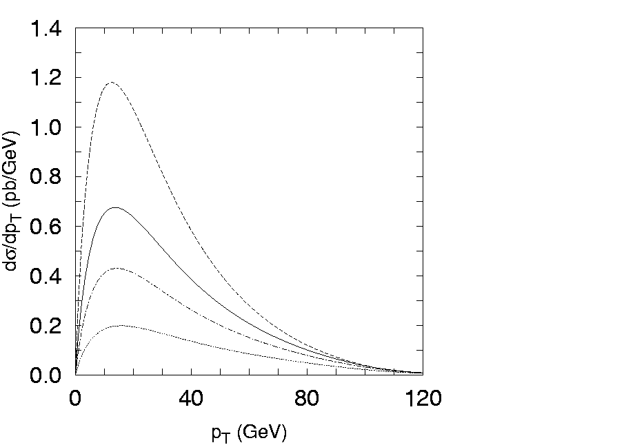
Figure 2: Differential cross section $d\sigma/dp_{T}$ for inclusive Higgs boson production at $\sqrt{s}=14$ TeV. The solid, dashed, dash-dotted and dotted lines correspond $m_{H}=125$ GeV, $m_{H}=100$ GeV, $m_{H}=150$ GeV and $m_{H}=200$ GeV, respectively.

In Figure 2 and 3 we display our prediction for the transverse momentum and rapidity distributions of the inclusive Higgs production at the LHC ($\sqrt{s}=14$ TeV). The calculations were done for four choices of the Higgs boson mass under interest in the Standard Model with default scale $\mu^{2}=m_{H}^{2}$. The solid, dashed, dash-dotted and dotted lines correspond $m_{H}=125$ GeV, $m_{H}=100$ GeV, $m_{H}=150$ GeV (where $WW$ decay channel is dominant) and $m_{H}=200$ GeV (above $WW$ and $ZZ$ decay tresholds), respectively. One can see that mass effects are present only at low $p_{T}<m_{H}$, whereas all curves practically coincide at large transverse momenta. We note that our predictions which correspond to the Higgs mass $m_{H}=125$ GeV slightly underestimate results obtained in the combined fixed-order + resummed approach [37]. In this approach fixed-order predictions (at LO or NLO level) and resummed ones (at NLL or NNLL level, respectively) have to be consistenly matched at moderate $p_{T}$. The NNLL + NLO results [25] are smaller than NLL + LO ones [24] by about $20$% at low transverse momenta. We see that our predictions lie below NNLL + NLO calculations by about $15$% in this kinematical region. Usage the doubly unintegrated gluon distributions results in more flat behaviour of the $p_{T}$-distribution [29] in comparison with both our and NNLL + NLO predictions.

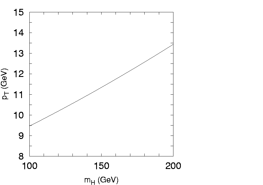
Figure 4: Location of the peak of the transverse momentum distributions for inclusive Higgs boson production as a function of Higgs mass at $\sqrt{s}=14$ TeV.

We note also that the peak in the transverse momentum distribution occurs at a smaller value of $p_{T}$ compared to the NNLL + NLO calculations. The location of this peak as a function of Higgs boson mass is shown in Figure 4. We find that at $m_{H}=125$ GeV the peak occurs at $p_{T}\sim 10$ GeV, whereas NNLL + NLO line peaks at $p_{T}\sim 15$ GeV [37]. The similar effect has been obtained [29] when doubly unintegrated gluon distributions were used.

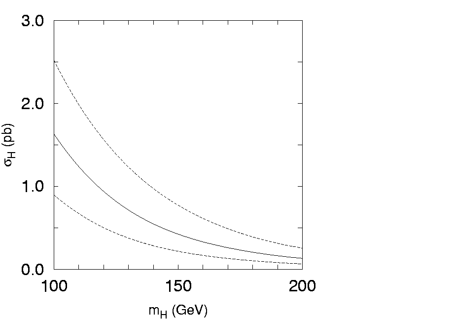
Figure 5: Total cross section of inclusive Higgs boson production as a function of Higgs mass at $\sqrt{s}=1.96$ TeV. The solid line corresponds to the default scale $\mu=m_{H}$, whereas upper and lower dashed lines correspond to the $\mu=m_{H}/2$ and $\mu=2m_{H}$ scales, respectively.

The total cross sections of the inclusive Higgs production at Tevatron ($\sqrt{s}=1.96$ TeV) and LHC conditions as function Higgs mass are plotted in Figure 5 and 6 in the mass range $m_{H}=100-200$ GeV. The solid lines are obtained by fixing both the factorization and renormalization scales at the default value $\mu=m_{H}$. In order to estimate the theoretical uncertainties in our predictions, we vary the unphysical parameter $\xi$ as indicated above. These uncertainties are presented by upper and lower dashed lines. We find that our default predictions agree very well with recent NNLO results [18]. For example, when Higgs boson mass is $m_{H}=120$ GeV, our calculations give $\sigma=0.84$ pb at Tevatron and $\sigma=35.9$ pb at LHC. However, the scale dependences are rather large. At LHC energy, it changes from about $20$% when $m_{H}=100$ GeV, to about $50$% when $m_{H}=200$ GeV. At Tevatron, it range from $40$% to $50$%, respectively. This fact indicates the necessarity of high-order corrections inclusion in the $k_{T}$-factorization formalism. But one should note that in the $k_{T}$-factorization the role of such correction is very different in comparison with the corrections in the collinear approach, since part of the standard high-order corrections are already included at LO level in $k_{T}$-factorization. At the same time the theoretical uncertainties of the collinear QCD calculations, after inclusion of both NNLO corrections and soft-gluon resummation at the NNLL level, are about $10$% in the low mass range $m_{H}<200$ GeV [18].

3.2 Higgs production in association with jets

Now we demonstrate how $k_{T}$-factorization approach can be used to calculate the semi-inclusive Higgs production rates. The produced Higgs boson is accompanied by a number of gluons radiated in the course of the gluon evolution. As it has been noted in Ref. [38], on the average the gluon transverse momentum decreases from the hard interaction block towards the proton. As an approximation, we assume that the gluon $k^{\prime}$ closest to the Higgs compensates the whole transverse momentum of the virtual gluon participating in the gluon fusion, i.e. ${\mathbf{k}^{\prime}}_{T}\simeq-{\mathbf{k}}_{T}$ (see Figure 1). All the other emitted gluons are collected together in the proton remnant, which is assumed to carry only a negligible transverse momentum compared to ${\mathbf{k}^{\prime}}_{T}$. This gluon gives rise to a final hadron jet with ${\mathbf{p}}_{{\rm jet}\,T}={\mathbf{k}^{\prime}}_{T}$.

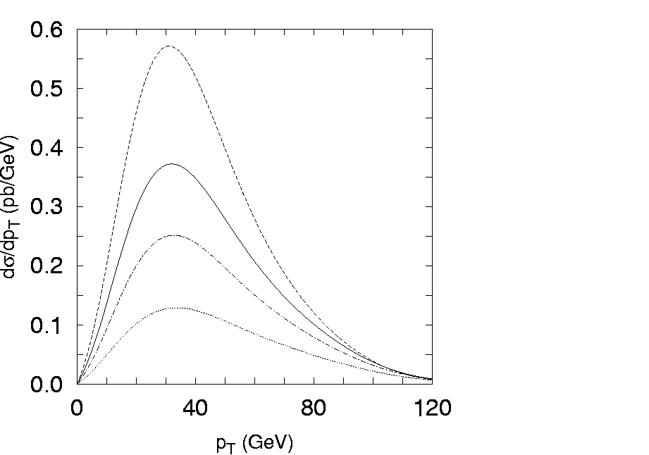
Figure 7: Differential cross section $d\sigma/dp_{T}$ for Higgs boson + one jet production at $\sqrt{s}=14$ TeV. The kinematical cut $|{\mathbf{p}}_{{\rm jet}\,T}|>20$ GeV was applied. All curves are the same as in Figure 2.

From the two hadron jets represented by the gluons from the upper and lower evolution ladder we choose the one carrying the largest transverse momentum, and then compute Higgs with an associated jet cross sections at the LHC energy. We have applied the usual cut on the final jet transverse momentum $|{\mathbf{p}}_{{\rm jet}\,T}|>20$ GeV. Our predictions for the transverse momentum distribution of the Higgs + one jet production are shown in Figure 7. As in the inclusive Higgs production case, we test four different $m_{H}$ values in the transverse momentum ditributions. All curves here are the same as in Figure 2. One can see the shift of the peak position in the $p_{T}$ distributions in comparison with inclusive production, which is direct consequence of the $|{\mathbf{p}}_{{\rm jet}\,T}|>20$ GeV cut. We note that the rapidity interval between the jet and the Higgs boson is naturally large. It is because there is angular ordering in the CCFM evolution, which is equivalent to an ordering in rapidity of the emitted gluons.

The investigation of the different azimuthal correlations between final particles in semi-inclusive Higgs production provides many interesting insights. In particular, studying of these quantities are important to clean separation of weak-boson fusion and gluon-gluon fusion contributions. To demonstrate the possibilities of the $k_{T}$-factorization approach, we present here the two azimuthal angle distributions. First, we calculate azimutal angle distribution between the Higgs boson and final jet transverse momenta in the Higgs + one jet production process. Second, we calculate azimuthal angle distributions between the two final jet transverse momenta in the Higgs + two jet production process. In this case the Higgs boson is centrally located in rapidity between the two jets and it is very far from either jet, and the kinematical cut $|{\mathbf{p}}_{{\rm jet}\,T}|>20$ GeV was applied for both final jets. We set no cuts on the jet-jet invariant mass. Our results are shown in Figure 8 and 9, respectively. Figure 8 demonstrated roughly the back-to-back Higgs + one jet production. In Figure 9 we obtained a dip at $90$ degrees in jet-jet azimuthal correlation, which is characteristic for loop-induced Higgs coupling to gluons [39]. The fixed-order perturbative QCD calculations of the $gg\to ggH$ subprocess give the similar result [16]. However, as it was already mentioned above, such calculations are very cumbersome even at leading order. The evaluation of the radiative corrections at ${\cal O}(\alpha_{s})$ to Higgs + two jet production would imply the calculation of up to hexagon quark loops and two-loop pentagon quark loops, which are at present unfeasible [20]. We note that contribution from the weak-boson fusion to the Higgs + two jet production has flat behavior of the jet-jet angular distribution [16, 20].

To illuminate the sensitivity of the Higgs production rates to the details of the unintegrated gluon distribution, we repeated our calculations for jet-jet angular correlations using J2003 set 2 gluon density [28] (dashed line in Figure 9). This density takes into account the singular and non-singular terms in the CCFM splitting function, where the Sudakov and non-Sudakov form factors were modified accordinly. We note that J2003 set 1 takes into account only singular terms. Both these sets describe the proton structure function $F_{2}(x,Q^{2})$ at HERA reasonable well. However, one can see the very large discrepancy (about order of magnitude) between predictions of J2003 set 1 and set 2 unintegrated gluon densities. The similar difference was claimed [28] for charm and bottom production at Tevatron also. This fact clearly indicates again that high-order corrections to the leading order $k_{T}$-factorization are important and should be developed for future applications.

4 Conclusions

We have considered the Higgs boson production via gluon-gluon fusion at high energy hadron colliders in the framework of the $k_{T}$-factorization approach. Our interests were focused on the Higgs boson total cross section and transverse momenta distributions at Tevatron and LHC colliders. In our numerical calculations we use the J2003 set 1 unintegrated gluon distribution, which was obtained recently from the full CCFM evolution equation.

We find that $k_{T}$-factorization gives the very close to NNLO pQCD results for the inclusive Higgs production total cross sections. It is because the main part of the high-order collinear pQCD corrections is already included in the $k_{T}$-factorization. Also we have demonstrated that $k_{T}$-factorization gives a possibility to investigate the associated Higgs boson and jets production in much more simple manner, than it can be done in the collinear factorization. Using some approximation, we have calculated transverse momentum distributions and investigated the Higgs-jet and jet-jet azimuthal correlations in the Higgs + one or two jet production processes. However, the scale dependence of our calculations is rather large (of the order of $20-50$%), which indicates the importance of the high-order correction within the $k_{T}$-factorization approach. These corrections should be developed and taken into account in the future applications.

We point out that in this paper we do not try to give a better prediction for Higgs production than the fixed-order pQCD calculations. The main advantage of our approach is that it is possible to obtain in straighforward manner the analytic description which reproduces the main features of the collinear high-order pQCD calculations. But in any case, the future experimental study of such processes at LHC will give important information about non-collinear gluon evolution dynamics, which will be useful even for leading-order $k_{T}$-factorization formalism.

5 Acknowledgements

The authors are very grateful to H. Jung for possibility to use the CCFM code for unintegrated gluon distributions in our calculations, for reading of the manuscript and useful discussion. We thank S.P. Baranov for encouraging interest and helpful discussions. N.Z. thanks P.F. Ermolov for support and the DESY directorate for the hospitality and support.

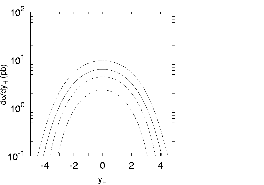
Figure 3: Differential cross section $d\sigma/dy_{H}$ for inclusive Higgs boson production at $\sqrt{s}=14$ TeV. All curves are the same as in Figure 2.

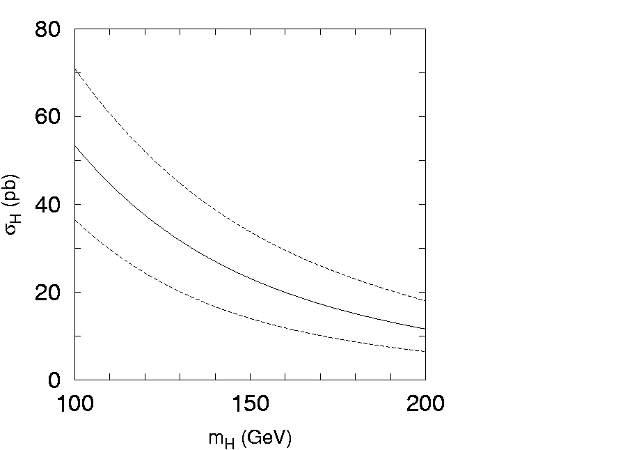
Figure 6: Total cross section of inclusive Higgs boson production as a function of Higgs mass at $\sqrt{s}=14$ TeV. All curves are the same as in Figure 5.

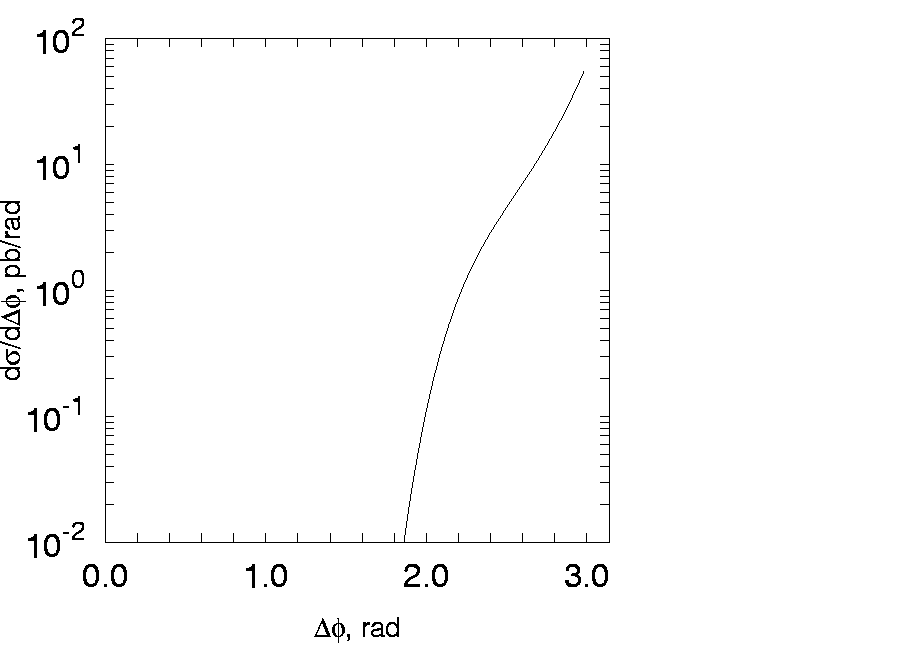
Figure 8: The Higg-jet azimutal angle distribution in the Higgs boson + one jet production at $\sqrt{s}=14$ TeV. The kinematical cut $|{\mathbf{p}}_{{\rm jet}\,T}|>20$ GeV was applied.

Figure 9: The jet-jet azimutal angle distribution in the Higgs boson + two jet production at $\sqrt{s}=14$ TeV. The kinematical cut $|{\mathbf{p}}_{{\rm jet}\,T}|>20$ GeV was applied for both jets. Solid and dashed lines correspond to the J2003 set 1 and J2003 set 2 unintegrated gluon distributions, respectively.

References

-
[1]
ATLAS Collaboration, Technical Design Report, Vol. 2, CERN/LHCC/99-15, 1999;
CMS Collaboration, Technical Proposal, CERN/LHCC/94-38, 1994. -
[2]
F. Wilczek, Phys. Rev. Lett. 39, 1304 (1977);
H.M. Georgi, S.L. Glashow, M.E. Machacek and D.V. Nanopoulos, ibid. Phys. Rev. Lett. 40, 692 (1978);
J.R. Ellis, M.K. Gaillard, D.V. Nanopoulos and C.T. Sachrajda, Phys. Lett. B83, 339 (1979);
T.G. Rizzo, Phys. Rev. D22, 178 (1980); D22, 1824 (1980). -
[3]
D. Graudenz, M. Spira and P.M. Zervas, Phys. Rev. Lett. 70, 1372 (1993);
M. Spira, A. Djouadi, D. Graudenz and P.M. Zervas, Nucl. Phys. B453, 17 (1995). -
[4]
N. Kauer, T. Plehn, D. Rainwater and D. Zeppenfeld, Phys. Lett. B503, 113 (2001);
T. Plehn, D. Rainwater and D. Zeppenfeld, Phys. Rev. D61, 093005 (2000);
D. Rainwater and D. Zeppenfeld, JHEP 9712, 005 (1997). -
[5]
V.N. Gribov and L.N. Lipatov, Yad. Fiz. 15, 781 (1972);
L.N. Lipatov, Sov. J. Nucl. Phys. 20, 94 (1975);
G. Altarelly and G. Parizi, Nucl. Phys. B126, 298 (1977);
Y.L. Dokshitzer, Sov. Phys. JETP 46, 641 (1977). -
[6]
E.A. Kuraev, L.N. Lipatov and V.S. Fadin, Sov. Phys. JETP 44, 443 (1976);
E.A. Kuraev, L.N. Lipatov and V.S. Fadin, Sov. Phys. JETP 45, 199 (1977);
I.I. Balitsky and L.N. Lipatov, Sov. J. Nucl. Phys. 28, 822 (1978). - [7] V.N. Gribov, E.M. Levin and M.G. Ryskin, Phys. Rep. 100, 1 (1983).
- [8] E.M. Levin, M.G. Ryskin, Yu.M. Shabelsky and A.G. Shuvaev, Sov. J. Nucl. Phys. 53, 657 (1991).
- [9] S. Catani, M. Ciafoloni and F. Hautmann, Nucl. Phys. B366, 135 (1991).
- [10] J.C. Collins and R.K. Ellis, Nucl. Phys. B360, 3 (1991).
-
[11]
M. Ciafaloni, Nucl. Phys. B296, 49 (1988);
S. Catani, F. Fiorani and G. Marchesini, Phys. Lett. B234, 339 (1990);
S. Catani, F. Fiorani and G. Marchesini, Nucl. Phys. B336, 18 (1990);
G. Marchesini, Nucl. Phys. B445, 49 (1995). - [12] J.R. Forshaw and A. Sabio Vera, Phys. Lett. B440, 141 (1998).
- [13] B.R. Webber, Phys. Lett. B444, 81 (1998).
- [14] G.P. Salam, JHEP 03, 009 (1999).
- [15] B. Andersson et al. (Small- Collaboration), Eur. Phys. J. C25, 77 (2002).
- [16] V. Del Duca, W. Kilgore, C. Olear, C. Schmidt and D. Zeppenfeld, Nucl. Phys. B616, 367 (2001); Phys. Rev. D67, 073003 (2003).
-
[17]
J.R. Ellis, M.K. Gaillard and D.V. Nanopoulos, Nucl. Phys.
B106, 292 (1976);
M.A. Shifman, A.I. Vainstein, M.B. Voloshin and V.I. Zakharov, Yad. Fiz. 30, 1368 (1979). -
[18]
R.V. Harlander and W.B. Kilgore, Phys. Rev. Lett. 88,
201801 (2002);
C. Anastasiou and K. Melnikov, Nucl. Phys. B646, 220 (2002);
V. Ravindran, J. Smith and W.L. van Neerven, Nucl. Phys. B665, 325 (2003). -
[19]
S. Dawson, Nucl. Phys. B359, 283 (1991);
A. Djouadi, M. Spira and P.M. Zervas, Phys. Lett. B264, 440 (1991). - [20] V. Del Duca, hep-ph/0312184.
- [21] J.C. Collins and D.E. Soper, Nucl. Phys. B193, 381 (1981); ibid. B213, 545 (1983); B197, 446 (1982).
- [22] J.C. Collins, D.E. Soper and G. Sterman, Nucl. Phys. B250, 199 (1985).
-
[23]
R.K. Ellis and S. Veseli, Nucl. Phys. B511, 649
(1998);
R.K. Ellis, D.A. Ross and S. Veseli, ibid. Nucl. Phys. B503, 309 (1997). -
[24]
S. Catani, E. D’Emilio and L. Trentadue, Phys. Lett. B211, 335 (1988);
R.P. Kauffmann, Phys. Rev. D45, 1512 (1992). - [25] D. de Florian and M. Grazzini, Phys. Rev. Lett. 85, 4678 (2000); Nucl. Phys. B616, 247 (2001).
- [26] A. Gawron and J. Kwiecinski, Phys. Rev. D70, 014003 (2004).
- [27] M.G. Ryskin, A.G. Shuvaev and Y.M. Shabelski, Phys. Atom. Nucl. 64, 120 (2001).
- [28] H. Jung, Mod. Phys. Lett. A19, 1 (2004).
- [29] G. Watt, A.D. Martin and M.G. Ryskin, Phys. Rev. D70, 014012 (2004), Erratum: ibid. D70, 079902 (2004), hep-ph/0309096.
-
[30]
B.R. Webber, Nucl. Phys. Proc. Suppl. C18, 38 (1991);
G. Marchesini and B.R. Webber, Nucl. Phys. B386, 215 (1992);
A. Gawron and J. Kwiecinski, Acta. Phys. Polon. B34, 133 (2003). - [31] M.A. Kimber, A.D. Martin and M.G. Ryskin, Phys. Rev. D63, 114027 (2001).
- [32] H. Jung, Comput. Phys. Comm. 143, 100 (2002).
- [33] F. Hautmann, Phys. Lett. B535, 159 (2002).
- [34] J. Andersen et al. (Small- Collaboration), Eur. Phys. J. C35, 67 (2004).
- [35] G.P. Lepage, J. Comput. Phys. 27, 192 (1978).
- [36] A.V. Lipatov and N.P. Zotov, hep-ph/0412275, submitted to Eur. Phys. J. C.
-
[37]
S. Catani, D. de Florian and M. Grazzini, Nucl. Phys. B596, 299 (2001);
JHEP 0201, 015 (2002);
G. Bozzi, S. Catani, D. de Florian and M. Grazzini, Phys. Lett. B564, 65 (2003);
S. Catani, D. de Florian, M. Grazzini and P. Nason, JHEP 0307, 028 (2003). - [38] S.P. Baranov and N.P. Zotov, Phys. Lett. B491, 111 (2000).
- [39] T. Plehn, D. Rainwater and D. Zeppenfeld, Phys. Rev. Lett. 88, 051801 (2002).