Cavendish-HEP-2005/01

January 2005

Gluon Distributions and Fits using Dipole Cross-Sections.

R.S. Thorne

Cavendish Laboratory, University of Cambridge,

Madingley Road, Cambridge, CB3 0HE, UK

I investigate the relationship between the gluon distribution obtained using a dipole model fit to low-$x$ data on $F_{2}(x,Q^{2})$ and standard gluons obtained from global fits with the collinear factorization theorem at fixed order. I stress the necessity to do fits of this type carefully, and in particular to include the contribution from heavy flavours to the inclusive structure function. I find that the dipole cross-section must be rather steeper than the gluon distribution, which at least partially explains why dipole model fits produce dipole cross-sections growing quite strongly at small $x$, while DGLAP based fits have valence-like, or even negative, small-$x$ gluons as inputs. However, I also find that the gluon distributions obtained from the dipole fits are much too small to match onto the conventional DGLAP gluons at high $Q^{2}\sim 50\rm GeV^{2}$, where the two approaches should coincide. The main reason for this discrepancy is found to be the large approximations made in converting the dipole cross-sections into structure functions using formulae which are designed only for asymptotically small $x$. The shortcomings in this step affect the accuracy of the extracted dipole cross-sections in terms of size and shape, and hence also in terms of interpretation, at all scales.

1 Introduction

In the description of structure function data the most conventional approach used is the collinear factorization theorem, where total cross-sections are determined in terms of parton distributions and hard parton cross-sections up to corrections of ${\cal O}(\Lambda_{QCD}^{2}/Q^{2})$, i.e. higher-twist corrections. The most complete method is to perform a so-called global fit [1, 2] to all data sensitive to parton distributions, so that the consistency of the fit to a variety of different data sets is guaranteed. This is currently done at either NLO or NNLO in the strong coupling $\alpha_{S}$ and appears to work very well. However, there are some indications [3] that the procedure is a little unreliable at small values of $x$ where a resummation of large $\ln(1/x)$ terms may be important [4], and by definition this whole approach fails at low values of $Q^{2}$ (where low appears to be somewhere from $0.5$ to $4\,\rm GeV^{2}$).

An alternative approach which circumvents the problem of low $Q^{2}$ and is particularly applicable to small $x$ is the colour dipole approach [5, 6, 7, 8]. Recently there have been a variety of fits, or at least comparisons, to small-$x$ structure function data using the dipole picture [9]-[16]. In this the free parameters of the fit are all mainly associated with the dipole cross-section, which it is very difficult to calculate from first principles but which may be modelled, with varying degrees, and different types of theoretical justification. If one also wants a finite photoproduction cross-section, a non-zero value must be chosen for the light-quark masses, appearing as a parameter in the dipole wavefunction which is calculated at LO, i.e. zeroth order in $\alpha_{S}$. It must be noted that in order to apply the approach to very low $Q^{2}$ one must assume that perturbation theory is valid and higher order QCD corrections to e.g. the photon wavefunction are meaningful and under control in this limit. This is yet to be proved. With this caveat in mind it is true that a variety of approaches to modelling the dipole cross-section can be made to match data very well.

Even though there is no essential connection, the dipole cross-section approach is often linked to, and used together with, the approaches which deal with parton saturation at small $x$. It is commonly believed that the complications of small $x$ and low $Q^{2}$ are entwined, with the assumed large parton distributions at small-$x$ leading to significant reduction of the evolution due to the mixing of leading-twist parton evolution with higher-twist multi-parton operators at low $Q^{2}$ [17, 18] (though it is fair to say that the values of $x$ and $Q^{2}$ which are relevant are not so commonly agreed). There has recently been a great deal of work attempting, as far as is possible, to calculate the dipole cross-sections within this framework of large densities and saturation (see e.g. [19], or for a slightly different viewpoint [20]), and many of the dipole fits, including some of the most successful, are based on these ideas. In some quarters this has led to very strong claims that saturation has been discovered. However, there is a conundrum. This picture of steeply growing parton distributions at small $x$ and low $Q^{2}$ tamed by saturation is in conflict with the conventional DGLAP fits which actually result in a small or even negative gluon (and consequently $F_{L}(x,Q^{2})$) at small $x$ and $Q^{2}$. It is essential to understand this before making any strong claims for saturation.

In this paper I will investigate the cause of this inconsistency. I will base this investigation very much on the completely standard assumption that the QCD factorization theory is completely reliable, correct and quantitative at fairly high $Q^{2}$ (as long as $x$ is not too small). Hence the parton distributions obtained from global fits must be quantitatively correct in this region. I will use the known relationships between the dipole cross-sections and standard parton distributions to work back from a fit to data performed in the dipole framework to obtain the corresponding partons. First, I will examine the question of whether a large/steep dipole cross-section actually means a large/steep gluon distribution, finding that the dipole cross-section is always steeper at small $x$ than its corresponding gluon distribution. This partially explains the differing conclusions obtained from the DGLAP and dipole approaches, but is not the whole story. In order to investigate the consistency of the two approaches I obtain a gluon distribution which evolves in the same way as a DGLAP gluon (at least for reasonably high $Q^{2}$) from a dipole model type fit to structure function data. I then make a comparison between the gluon distribution obtained at fairly high $Q^{2}$ from this dipole model fit and the gluon from a standard set of parton distributions. This gives strong evidence as to whether dipole motivated fits are truly quantitative, and whether the results from these fits are to be taken seriously in detail. I find that the comparison between the two illustrates a serious discrepancy, and point out that the reason for this discrepancy is the approximation inherent in the LO dipole wavefunctions. I conclude that this result casts doubt on whether we should indeed treat the results of fits to HERA data using the dipole picture as telling us anything truly quantitative, and I explain my reservations. Improvements in the quantitative form of the gluon distributions obtained from dipole model inspired fits rely mainly on increasing the precision of the wavefunctions used to obtain the structure functions from the dipole cross-section.

2 The Relationship Between The Dipole Cross-Section and The Gluon Distribution

The relationship between the gluon distribution and the dipole cross-section was essentially worked out as soon as the dipole approach was proposed [7], but it is nicely discussed in a pedagogical manner in [21] which explicitly shows the relationship between the dipole picture and the $k_{T}$-factorization theorem [22] at LO, and also shows how this relationship breaks down beyond LO. My discussion partly follows this paper. The diagrams contributing to deep inelastic scattering at LO are shown below, where the incoming gluons have finite transverse momentum $\vec{k}$.

Within the LO $k_{T}$-factorization theory we can write, for example, the longitudinal $\gamma^{\star}p$ cross-section as

$$\sigma_{L}(x,Q^{2})\propto\int_{0}^{1}dz[z(1-z)]^{2}\int\frac{d^{2}k}{k^{4}}\int d^{2}p\biggl{(}\frac{1}{\hat{Q}^{2}+p^{2}}-\frac{1}{\hat{Q}^{2}+(p+k)^{2}}\biggr{)}^{2}f(x_{g},k^{2})$$ (1)

where $f(x_{g},k^{2})$ is the unintegrated gluon distribution and $\hat{Q}^{2}=z(1-z)Q^{2}$. A similar result, but slightly more complicated formula, also holds for $\sigma_{T}$. Staying at strictly LO in $\ln(1/x)$ in the $k_{T}$-factorization theory, we work in the limit $x\to 0$, i.e. since

$$\ln(x)=\ln(x_{g})+\ln\bigl{(}\hat{Q}^{2}/(\hat{Q}^{2}+\hat{k}^{2}+(p^{\prime})^{2})\bigr{)},$$ (2)

where $\vec{p}^{\prime}=\vec{p}-(1-z)\vec{p}$, we simply make the identity $x=x_{g}$. In this limit Eq.(1) can be simplified significantly. Integrating over $z$ and $p$, which in this limit does not involve $f(x,k^{2})$ we have the standard $k_{T}$-factorization expression, which can be written in terms of the structure function as

$$F_{L}(x,Q^{2})=\int\frac{dk^{2}}{k^{2}}\,\frac{\alpha_{S}2N_{f}}{6\pi}\,\,h_{L}(k^{2}/Q^{2})f(x,k^{2}).$$ (3)

Taking the double Mellin transformation $\int dQ^{2}Q^{2-2\gamma}$ and $\int dx\,x^{N}$ we have the familiar expression.

$$\tilde{F}_{L}(N,\gamma)=\frac{\alpha_{S}2N_{f}}{6\pi}\,\tilde{h}_{L}(\gamma)\tilde{f}(N,\gamma)/\gamma\equiv\frac{\alpha_{S}2N_{f}}{6\pi}\,\tilde{h}_{L}(\gamma)\tilde{g}(N,\gamma),$$ (4)

where $g(x,Q^{2})=\int_{0}^{Q^{2}}\frac{dk^{2}}{k^{2}}f(x,k^{2})$ is the integrated gluon distribution, and $\tilde{h}_{L}(\gamma)$ is the longitudinal impact factor first calculated in [23]. An exactly analogous expression can be calculated for $F_{2}(x,Q^{2})$, though it is usually expressed in terms of $dF_{2}/d\ln Q^{2}$ in order to preserve finiteness in the infrared limit, i.e.

$$\frac{dF_{2}(x,Q^{2})}{d\ln Q^{2}}=\int\frac{dk^{2}}{k^{2}}\,\frac{\alpha_{S}2N_{f}}{6\pi}\,\,h_{2}(k^{2}/Q^{2})f(x,k^{2}).$$ (5)

If the gluon distribution can be expressed in the simple form $g(N,Q^{2})\sim(Q^{2})^{\gamma(\alpha_{S},N)}$ this leads to

$$F_{i}(N,Q^{2})=\frac{\alpha_{S}2N_{f}}{6\pi}h_{i}(\gamma(\alpha_{S},N))g(N,Q^{2})$$ (6)

which taking the inverse Mellin transformation becomes

$$F(x,Q^{2})=\frac{\alpha_{S}2N_{f}}{6\pi}h(\gamma(\alpha_{S},\ln(1/x)))\otimes g(x,Q^{2}).$$ (7)

This is the standard result of the LO in $\ln(1/x)$ $k_{T}$-factorization theorem. Contrary to what seems to be common belief, the $k_{T}$-factorization theorem is well defined beyond this order. Indeed, in [23] it is demonstrated that $k_{T}$-factorization may be thought of as simply a reordering of the calculations performed within the collinear factorization theorem, and as such it is as well defined as collinear factorization, i.e. to all orders at leading twist.

There is an alternative way to proceed from the starting point of Eq.(1). By using the identity

$$\frac{1}{\hat{Q}^{2}+p^{2}}=\frac{1}{2\pi}\int d^{2}r\exp(ip\cdot r)K_{0}(\hat{Q}r)$$ (8)

and integrating over $p^{2}$, using the independence of $x_{g}$ on $p^{2}$ in the $x\to 0$ limit, one can equivalently write

$$\sigma=\frac{4\pi^{2}}{3}\int_{0}^{1}dz\int d^{2}r|\Psi(r,z,Q)|^{2}\int\frac{dk^{2}}{k^{4}}\alpha_{S}f(x,k^{2})(1-J_{0}(kr)).$$ (9)

$|\Psi(r,z,Q)|^{2}$ is the probability for a photon of virtuality $Q^{2}$ to fluctuate into a a dipole pair, as calculated in [7], and is explicitly

$$|\Psi_{T}(r,z,Q)|^{2} = \frac{6\alpha}{4\pi^{2}}\sum_{f}e_{f}^{2}\bigl{(}[z^{2}+(1-z)^{2}]\epsilon^{2}K_{1}^{2}(\epsilon r)+m_{f}^{2}K_{0}^{2}(\epsilon r)\bigr{)}$$ (10)

$$|\Psi_{L}(r,z,Q)|^{2} = \frac{6\alpha}{\pi^{2}}\sum_{f}e_{f}^{2}\bigl{(}Q^{2}[z^{2}+(1-z)^{2}]K_{0}^{2}(\epsilon r)\bigr{)},$$ (11)

where $\epsilon^{2}=z(1-z)Q^{2}+m_{f}^{2}$, and $m_{f}$ is the mass of a given quark flavour. Hence, Eq.(9) can be interpreted as

$$\sigma=\int_{0}^{1}dz\int d^{2}r|\Psi(r,z,Q)|^{2}\hat{\sigma}(x,r^{2}),$$ (12)

where

$$\hat{\sigma}(x,r^{2})=\frac{4\pi^{2}}{3}\int\frac{dk^{2}}{k^{4}}\alpha_{S}f(x,k^{2})(1-J_{0}(kr))$$ (13)

may be associated with the dipole-proton cross-section. In the LO $\ln(1/x)$ limit this and Eq.(4) are really equivalent, but because in Eq.(4) we have reference to the gluon density, which we think of as evolving perturbatively, and have an explicit factor of $\alpha_{S}$, we think of this equation only having validity for $Q^{2}\gg\Lambda_{QCD}^{2}$. In principle the same issues exist for Eq.(12), with $\hat{\sigma}(x,r^{2})$ depending on both the (unintegrated) gluon distribution and $\alpha_{s}$, as seen in Eq.(13). However, ignoring these complications and proposing models for $\hat{\sigma}(x,r^{2})$ valid for all $r$, Eq.(12) is often used down to the photoproduction limit of $Q^{2}=0$, albeit requiring regularization from finite light quark masses. However, as discussed in [21] the form of the expression in Eq.(12) is definitely not preserved beyond the leading $\ln(1/x)$ limit, with inclusion of real gluon kinematics spoiling the diagonalization in the transverse size $\vec{r}$ of the incoming and outgoing dipoles.

At LO we can investigate what the equivalence of the two approaches tells us. In the standard $k_{T}$-factorization theorem approach $F_{i}(N,Q^{2})$ is given by Eq.(6), or its equivalent for $d\,F_{2}(N,Q^{2})/d\ln Q^{2}$. Taking the Mellin transformation with respect to $x$ of the intermediate expression Eq.(9) and using the equivalence we obtain

$$F_{i}(N,Q^{2})=\frac{\alpha_{S}2N_{f}}{6\pi}h_{id}(\gamma(\alpha_{S},N))h_{dg}(\gamma(\alpha_{S},N))g(N,Q^{2})\equiv\frac{\alpha_{S}2N_{f}}{6\pi}h_{i}(\gamma(\alpha_{S},N))g(N,Q^{2}),$$ (14)

where $h_{id}(\gamma)$ comes from the probability of the photon splitting to the dipole, while $h_{dg}(\gamma)$ comes from the relationship between the dipole cross-section and the gluon distribution in Eq.(13). Therefore, the effective coefficient function for the hard cross-section $h_{i}(\gamma(\alpha_{S},N))$ can be interpreted as the product of a photon-dipole coefficient function $h_{id}(\gamma(\alpha_{S},N))$ and a dipole-gluon coefficient function $h_{dg}(\gamma(\alpha_{S},N))$, both of which are calculable. For the more phenomenologically interesting case of $dF_{2}/d\ln Q^{2}$ we find from a straightforward calculation

$$h_{dg}(\gamma) = \frac{4^{\gamma}\Gamma(1+\gamma)}{(1-\gamma)\Gamma(2-\gamma)},$$ (15)

$$h_{2d}(\gamma) = \frac{(1+3/2\gamma-3/2\gamma^{2})}{1-\gamma}\frac{4^{-\gamma}\Gamma^{4}(2-\gamma)\Gamma^{2}(1+\gamma)}{\Gamma(4-2\gamma)\Gamma(2+2\gamma)},$$ (16)

$$h_{2g}(\gamma) = \frac{3/2(2-3\gamma+3\gamma^{2})}{3-2\gamma}\frac{\Gamma^{3}(1+\gamma)\Gamma^{3}(1-\gamma)}{\Gamma(2+2\gamma)\Gamma(2-2\gamma)},$$ (17)

and the equivalence in Eq.(14) is easily verified.

The implications of this turn out to be rather interesting. Each of these effective coefficient functions can be expanded as a power series in $\gamma$ about $\gamma=0$, where each has been normalized so that $h(0)=1$. For $dF_{2}/d\ln Q^{2}$ we obtain,

$$h_{2}(\gamma(\bar{\alpha}_{S}/N))=1+2.17\gamma+2.30\gamma^{2}+5.07\gamma^{3}+3.58\gamma^{4}+8.00\gamma^{5}+\cdots$$ (18)

In order to interpret this we need to know more about $\gamma$. Strictly speaking, these expressions are all derived within the LO in $\ln(1/x)$ framework. In this case the gluon anomalous dimension is given by the LO BFKL equation. This results in the power-series expansion

$$\gamma(\alpha_{S}/N)=\frac{\bar{\alpha}_{S}}{N}+2.4(\frac{\bar{\alpha}_{S}}{N})^{4}+2(\frac{\bar{\alpha}_{S}}{N})^{6}+17(\frac{\bar{\alpha}_{S}}{N})^{7}+\cdots,$$ (19)

where $\bar{\alpha}_{S}=(3/\pi)\alpha_{S}$. In $x$ space this results in a splitting function

$$xP_{gg}(\alpha_{S},x)=\bar{\alpha}_{S}+2.4(\frac{\bar{\alpha}^{4}_{S}\ln^{3}(1/x)}{3!})+2(\frac{\bar{\alpha}_{S}^{6}\ln^{5}(1/x)}{5!})+17(\frac{\bar{\alpha}^{7}_{S}\ln^{6}(1/x)}{6!})+\cdots.$$ (20)

This steep growth of $xP_{gg}$ as $x$ decreases leads to a quickly increasing small-$x$ gluon distribution as $Q^{2}$ increases. However, substituting $\gamma(\alpha_{S}/N)$ into Eq.(18) we see that the effective coefficient function also grows quickly at small $N$, or equivalently at small $x$, and consequently $d\,F_{2}(x,Q^{2})/d\ln Q^{2}$ grows quite a lot more quickly than $g(x,Q^{2})$ with decreasing $x$.

Expanding the other expressions in Eq.(17) in powers of $\gamma$ we obtain

$$h_{dg}(\gamma(\bar{\alpha}_{S}/N)) = 1+2.23\gamma+3.49\gamma^{2}+3.95\gamma^{3}+4.22\gamma^{4}+4.06\gamma^{5}+\cdots$$ (21)

$$h_{2d}(\gamma(\bar{\alpha}_{S}/N)) = 1-0.07\gamma-1.05\gamma^{2}+3.77\gamma^{3}-4.94\gamma^{4}+6.53\gamma^{5}-\cdots.$$ (22)

Hence, $h_{dg}(\gamma)$ has a power series expansion in which all the coefficients are positive, and of rather similar size to those in the expansion of $h_{2}(\gamma)$, whereas $h_{2d}(\gamma)$ has a series expansion where the first two terms are small and negative, and higher terms oscillate. This has an obvious consequence. To a reasonable approximation all the small-$x$ enhancement of $dF_{2}/d\ln Q^{2}$ relative to $g(x,Q^{2})$ is generated by the dipole-gluon cross-section, which is therefore itself steep relative to the gluon. In the final conversion from the dipole cross-section to $dF_{2}/d\ln Q^{2}$ there is little change in $x$ dependence.

Figure 1: $\hat{\sigma}(x,r^{2})$ and $xg(x,Q^{2})$ obtained from the original Golec-Biernat Wüsthoff dipole model [9]. $xf_{g}(x,k^{2})$ has the same type of shape as $xg(x,Q^{2})$. A flattening dipole at small $x$ requires a valence-like integrated or unintegrated gluon distribution.

In practice the LO BFKL prediction for the gluon is not really used in any realistic dipole model fits to data. It predicts a power-like behaviour at small $x$ of $x^{\lambda}$, where $\lambda=4\ln(2)\bar{\alpha}_{S}=2.65\alpha_{S}$, whereas the sort of power-like behaviour used is $\lambda\sim 0.25-0.3$. This means an effective value of $\alpha_{S}=0.1$ which is extremely low for scales of a few GeV, where $\alpha_{S}=0.2-0.3$, which is where the data exist. Hence some models use behaviour implied by higher order corrections within the BFKL framework (see e.g. the calculation in [24]), and others just use models where the gluon is more closely associated with standard LO or NLO in $\alpha_{S}$ perturbative QCD. Some are more ad hoc. This departure from the LO $k_{T}$-factorization is already a deviation from the theoretical framework within which the simple dipole picture is valid, but I will essentially disregard this particular issue throughout this paper. Whatever the inspiration for the (unintegrated) gluon distribution, in order to match even the most qualitative trends of the data one needs a gluon distribution that increases quickly with $Q^{2}$ at small $x$, and every model ultimately has an effective $\gamma(\alpha_{S},N)$ that grows quickly at small $N$ and equivalently at small $x$. Therefore, the general conclusion on the role of the effective coefficient functions made above is always true. Since $\gamma$ is positive and increasing at small $x$, $dF_{2}/d\ln Q^{2}$ is always steeper in $x$ than $g(x,Q^{2})$, and this relative steepness is always associated with the step taking one from the gluon to the dipole cross-section, with the step taking one from the dipole cross-section to the physical structure function being largely unimportant as far as the shape is concerned.

This conclusion does not seem to have been made previously, but it is easy to demonstrate using the very simple dipole model proposed in [9]. In this case the dipole cross-section is given by

$$\hat{\sigma}(x,r^{2})=\sigma_{0}(1-\exp(r^{2}/4(x_{0}/x)^{\lambda})),$$ (23)

where, for the case of the realistic fit which includes charm as a parton rather than simply using three light flavours, the parameters obtained from the best fit were $\sigma_{0}=29.2mb,x_{0}=4\times 10^{-5},\lambda=0.28$. This cross-section clearly saturates at large enough $r$ or small enough $x$. Using the relationship between the dipole cross-section and the unintegrated gluon distribution it is straightforward to obtain

$$f_{g}(x,k^{2})=\frac{3\sigma_{0}}{4\pi^{2}\alpha_{S}}k^{4}(x/x_{0})^{\lambda}e^{-k^{2}(x/x_{0})^{\lambda}},$$ (24)

and this expression is indeed used in [10]. Thus, whilst $\hat{\sigma}(x,r^{2})\to\sigma_{0}$ as $x\to 0$, $f_{g}(x,k^{2})\to 0$ as $x\to 0$, i.e. it has a valencelike behaviour $f_{g}(x,k^{2})\sim x^{0.28}$ as $x\to 0$. Using the leading twist relationship between the unintegrated and integrated gluon distribution, $g(x,Q^{2})=\int_{0}^{Q^{2}}\frac{dk^{2}}{k^{2}}f(x,k^{2})$, and using fixed coupling (the general result does not depend on this), we obtain

$$xg(x,Q^{2})=\frac{3\sigma_{0}}{4\pi^{2}\alpha_{S}}\biggl{[}-Q^{2}e^{-Q^{2}(x/x_{0})^{\lambda}}+(x_{0}/x)^{\lambda}(1-e^{-Q^{2}(x/x_{0})^{\lambda}})\biggr{]},$$ (25)

which also behaves like $x^{0.28}$ as $x\to 0$. This is slightly reminiscent of the valencelike gluons obtained in global fits, except that the valence-like behaviour will always set in at low enough $x$ in this model (though extremely low $x$ for high $Q^{2}$), whereas in the DGLAP approach the valencelike behaviour soon disappears with evolution to higher $Q^{2}$. The behaviour of the dipole cross-section at large $r$ is compared to that of $g(x,Q^{2})$ at low $Q^{2}$ in Fig. 1, and one clearly sees that the eventual flattening of $\hat{\sigma}(x,r^{2})$ at low $x$ is accompanied by a distinct turnover in $g(x,Q^{2})$, with the maximum as high as $x\sim 0.005$ at $Q^{2}=0.5\rm GeV^{2}$.

It is certainly reasonable to argue that the simple relationship between the integrated and unintegrated gluons is not meant to be used in this case, since higher twist corrections to the gluon will be important. However, again this takes us beyond the regime where the strict equivalence between the dipole picture and the rigorously defined $k_{T}$-factorization theorem is valid. Also, even if one doubts the result presented in terms of $g(x,Q^{2})$, it is certainly the case that $f_{g}(x,k^{2})$ is valencelike. Hence, this simple example shows that the dipole cross-section becoming large at a small value of $x$ does not necessarily mean that the gluon at this value of $x$ is also large. This perhaps clouds the issue of what saturation actually means, i.e. does it have to mean a large parton density. However, it might also go some way towards explaining why fits including saturation corrections seem to be successful, while standard DGLAP fits produce very small (or negative) gluons, and small $x$ and $Q^{2}$.

In order to provide a definitive answer to this apparent contradiction it is necessary to undertake some rather more precise work. Although the original Golec-Biernat Wüsthoff dipole model was successful with the HERA data available at the time, it now produces a qualitatively good fit at best. And some of the more recent fits are direct attempts to improve it, e.g. [13]. Thus in order to make quantitative conclusions it is necessary to relate the gluon distribution and dipole cross-section from a genuinely good fit to current data.

3 The Model for the Gluon Distribution

In order to make a detailed investigation I will work on the principle that reasonably high $Q^{2}$ the gluon distribution will behave exactly according to standard fixed order DGLAP evolution. Hence, I propose a simplified model for the gluon which accurately represents this but contains a minimum of parameters. I will then use the exact relationship between the unintegrated gluon distribution and the dipole cross-section in Eq.(13), along with the standard identity, $f_{g}(x,k^{2})=\biggl{(}\frac{d\,g(x,Q^{2})}{d\ln Q^{2}}\biggr{)}_{Q^{2}=k^{2}}$, valid at leading twist, in order to obtain the correct expression for $\hat{\sigma}(x,r^{2})$. In the small $r^{2}$ limit $\hat{\sigma}(x,r^{2})$ may be written as

$$\hat{\sigma}(x,r^{2})=\frac{4\pi^{2}}{3}r^{2}\int\frac{dk^{2}}{k^{2}}\alpha_{S}f(x,\mu^{2})\sim\frac{\pi^{2}\alpha_{S}}{3}r^{2}g(x,\mu^{2}),$$ (26)

where $\mu^{2}=A/r^{2}$ [25]. The constant $A$ depends on the precise behaviour of the gluon, but it is always the case that $A\approx 10$. It should not be used as a free parameter in a fit. This expression is sometimes used to relate the gluon distribution and dipole cross-section. However, it is only ever approximate and only reasonable for very small $r$. The completely correct Eq.(13) should really be used if one is going into the regime of large $r$ and or small $Q^{2}$ and $k^{2}$.

In order to attempt to obtain a matching between the dipole model gluon distribution and a DGLAP one at large $Q^{2}$ I define a gluon distribution which behaves like a conventional global fit gluon at high scales. I note that to a very good approximation at LO in $\alpha_{S}$ the gluon anomalous dimension is $\gamma_{gg}(\alpha_{s}(Q^{2}),N)=\bar{\alpha}_{s}(Q^{2})(1/N-1)$, only differing from this approximate form significantly at very high $N$. Hence, the LO evolution is given by this anomalous dimension to a good accuracy except for fine details at the highest $x$. Furthermore, apparently by accident the NLO correction to gluon evolution is very small, the coefficient of a possible term of $1/N^{2}$ happening to be zero. It was shown in [26] that for a flat input at scale $Q_{0}^{2}$ the solution to the evolution equation for $Q^{2}>Q_{0}^{2}$ using this anomalous dimension is roughly

$$xg(x,Q^{2})\propto I_{0}\biggl{(}\!\biggl{(}2.4\zeta_{0}\log\biggl{(}\frac{\log((Q^{2})/\Lambda_{QCD}^{2})}{\log((Q_{0}^{2})/\Lambda_{QCD}^{2})}\biggr{)}\!\biggr{)}^{0.5}\biggr{)}\exp\biggl{(}\!-1.5\log\biggl{(}\frac{\log((Q^{2})/\Lambda_{QCD}^{2})}{\log((Q_{0}^{2})/\Lambda_{QCD}^{2})}\biggr{)}\!\biggr{)},$$ (27)

where $\zeta_{0}=\ln(x_{0}/x)$, and strictly speaking $x_{0}$ is the value of $x$ above which the flat input gluon distribution falls away to zero, i.e. $g(x,Q_{0}^{2})\propto\Theta(x_{0}-x)$.

This is a very good starting point for a more realistic gluon distribution. The main modification to be made is to round off the high-$x$ behaviour to something more like $(1-x)^{5}$ rather than a $\Theta$ function at $x_{0}$, and to take account of this in the evolution. Also, I want a gluon that can be used all the way down to $Q^{2}=0$ rather than stopping at some input scale, and which tends smoothly to a flat behaviour in $x$ as $Q^{2}\to 0$. This is achieved by modifying Eq.(27) to

$$xg(x,Q^{2}) = A\biggl{(}\frac{5}{5+\zeta}\biggr{)}^{2}\exp\biggl{(}-1.5\log\biggl{(}\frac{\log((Q^{2}+Q_{0}^{2})/\Lambda_{QCD}^{2})}{\log((Q_{0}^{2})/\Lambda_{QCD}^{2})}\biggr{)}\biggr{)}$$

$$\times\biggl{(}I_{0}\biggl{(}2.4\biggl{(}\frac{\eta^{2}(1-\exp(-\eta/4))}{\eta+2.3}(1-\exp(-\eta))^{4}\log\biggl{(}\frac{\log((Q^{2}+Q_{0}^{2})/\Lambda_{QCD}^{2})}{\log((Q_{0}^{2})/\Lambda_{QCD}^{2})}\biggr{)}\biggr{)}^{0.5}\biggr{)}-1\biggr{)}.$$

$A\biggl{(}\frac{5}{5+\eta}\biggr{)}^{2}$ is the input, with $A$ the normalization. This is simply an empirical modification of an original formula which was theoretically correct in a slightly idealized framework; and for moderate and high $Q^{2}$, i.e. above a few $GeV^{2}$, the gluon does behave very similarly indeed to the standard DGLAP gluons coming from global fits. $\Lambda_{QCD}=0.12\rm GeV$, which for the one-loop coupling gives $\alpha_{S}(M_{Z}^{2})=0.118$, i.e. roughly the correct value, and hence it gets the speed of evolution correct. $Q_{0}^{2}=0.5\rm GeV^{2}$, and marks the transition scale around which perturbative evolution is beginning to break down. $Q_{0}^{2}$ and the input shape $(5/(5+\eta))^{2}$ are chosen to give roughly the correct phenomenological shape in $x$ and $Q^{2}$ for the lowish $Q^{2}$ gluon, but neither is at all fine-tuned. $Q_{0}^{2}$ takes on a perfectly typical value for the scale of nonperturbative physics. It clearly serves the function of slowing the evolution $Q^{2}\sim Q_{0}^{2}$, but does this in an $x$-independent way. I only make the change $Q^{2}\to Q^{2}+Q_{0}^{2}$, independent of any consideration of $x$. This model of the gluon is not therefore inspired at all by the idea of slowing evolution associated with high parton densities at small $x$, and does not contain saturation effects.

This expression for the gluon is converted into a dipole cross-section using

$$\hat{\sigma}(x,r^{2})=\frac{4\pi^{2}}{3}\int\frac{dk^{2}}{k^{4}}\alpha_{S}(k^{2})f(x,k^{2})(1-J_{0}(kr)),$$ (29)

where for consistency $\alpha_{S}(\mu^{2})$ is also slowed at low scales with the same regularization as the gluon.

$$\alpha_{S}(\mu^{2})=\frac{4\pi}{\beta_{0}\log((\mu^{2}+Q_{0}^{2})/\Lambda_{QCD}^{2})}.$$ (30)

The results of this paper are largely insensitive to the details of how the low scale coupling is regularized. The resulting dipole cross-section is then put into a fit to data. The normalization $A$ is the only really free parameter associated with the gluon in this fit.

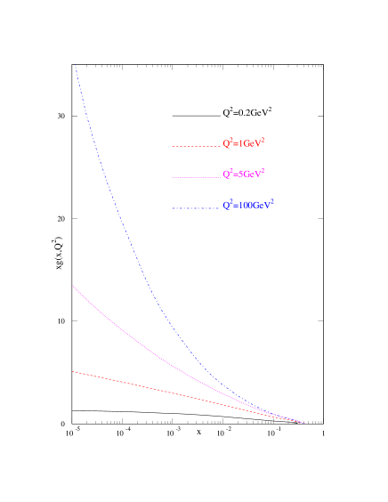
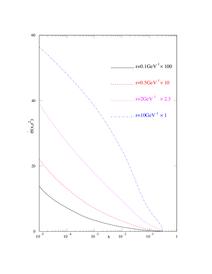
Figure 2: Comparison of $xg(x,Q^{2})$ in my model at various $Q^{2}$ with the corresponding $\hat{\sigma}(x,r^{2})$ at various $r$. The normalization is determined by the best fit to data.

Since the shape of the gluon has now been determined, we can investigate the relative shapes of the gluon distribution and the dipole cross-section without having to know the value of $A$. This is illustrated in Fig. 2, where we see $xg(x,Q^{2})$ and $\hat{\sigma}(x,r^{2})$ for a variety of values of $Q^{2}$ and $r$. For the largest value of $Q^{2}$ and correspondingly the smallest value of $r$ both $g(x,Q^{2})$ and $\hat{\sigma}(x,r^{2})$ rise steeply at small $x$, and it is difficult to see any particular difference in shape. However, at the two lower values of $Q^{2}$, $1\rm GeV^{2}$ and $0.2\rm GeV^{2}$, $g(x,Q^{2})$ is clearly flattening out, and is rising very slowly indeed in the latter case. For the two larger values of $r$, $2\rm GeV^{-1}$ and $10\rm GeV^{-1}$ (which would naively correspond to $Q^{2}$ of about $2.5\rm GeV^{2}$ and $0.1\rm GeV^{2}$ respectively), $\hat{\sigma}(x,r^{2})$ is clearly still rising steeply, and it is in this regime, which is where any saturation effects are supposed to be large, that the influence of the effective dipole-gluon coefficient function is clearly seen. It would seem easy to believe that saturation were occuring due to a large dipole cross-section, but seems less plausible that this could be interpreted as being due to a steeply growing density of gluons.

4 Details of the Fit

There are a number of modifications required compared to the standard approach to fits to data made within the dipole picture in order to get a truly quantitative comparison to the conventional DGLAP approach. One extremely important issue is the treatment of heavy quarks, i.e. charm and bottom. These are often ignored in dipole fits. This is certainly excusable for the bottom contribution, which only really turns on above $Q^{2}=m_{b}^{2}\approx 20\rm GeV^{2}$, and carries a charge weighting of 1/9. However, charm contributes about $40\%$ of $dF_{2}/d\ln Q^{2}$ for $Q^{2}>m_{c}^{2}$, i.e. it turns on from zero to a very sizeable contribution indeed somewhere in the middle of the dipole regime, and to ignore it is ludicrous.

However, the charm contribution to inclusive $F_{2}(x,Q^{2})$ is often left out in dipole model fits. In the original [9] fits, two fits were made, with and without charm. The latter actually gave a worse fit, and the form of the dipole cross-section changed, the saturation parameter $x_{0}$, i.e the value of $x$ at which saturation becomes very important at $Q^{2}=1\rm GeV^{2}$, changed from $x_{0}=3\times 10^{-4}$ without charm to $x_{0}=4\times 10^{-5}$ with charm, and the overall magnitude of the dipole cross-section decreased significantly, to about $60\%$ the previous value except at very large $r$ or extremely small $x$. Neither of these results is surprising. If one is missing up to $40\%$ of $dF_{2}/d\ln Q^{2}$ one would expect an enhancement of $\hat{\sigma}(x,r^{2})$ and $g(x,Q^{2})$ of up to $1.67$. Since the leading saturation corrections are $\propto g^{2}(x,Q^{2})$, one would then expect the saturation effects to be much exaggerated when charm is absent, as seen. For some reason the results of the dipole fits are habitually cited using the parameter values from the fits with charm absent. These parameters are simply wrong, and should not be used. Moreover, they clearly suggest that saturation effects are quite a lot larger than the results obtained from the more correct dipole fits.

In order to investigate the importance of the charm contribution to inclusive $F_{2}(x,Q^{2})$ I tried performing global fits with this contribution set to zero, i.e. mimicking what is done in many dipole fits. The procedure for the fit was exactly as in the usual MRST fits other than this one modification. It seems obvious that, in order to counter the absence of a large part of the theoretical contribution, the gluon must get bigger at small $x$ to increase evolution. However, the gluon cannot simply get bigger everywhere because of the momentum sum rule, so it seemed very likely that $\alpha_{S}$ would also have to get bigger to also try to speed up evolution. The results were broadly in line with these expectations, but were rather dramatic in other senses. The main point to note is that the quality of the global fit performed in this manner is terrible, with $\chi^{2}=4000$ for $2000$ points, twice that of the normal global fit. At small $x$ it is impossible to get $dF_{2}/d\ln Q^{2}$ consistently correct at all $x$ and $Q^{2}$. At low $Q^{2}$ the gluon wishes to be not too much bigger than normal, charm not yet being so important in the evolution. However, such a low $Q^{2}$ gluon is then much too small to get evolution correct at higher $Q^{2}$. Conversely a gluon large enough for the higher $Q^{2}$ data is far too big for the evolution at low $Q^{2}$. There is no way around this within the factorization theorem. Also the increased $\alpha_{S}$ needed to help the small $x$ fit makes the fit to the rest of the data much worse. The quality of the fit breaks down everywhere.

This slightly surprising result may be viewed as a very positive one for collinear factorization. It shows that NLO and NNLO DGLAP calculations are good enough and constraining enough to determine that charm has to be there, and to constrain its mass quite accurately, even without using any data directly sensitive to charm. This suggests one should be suspicious of good qualitative results obtained from calculation where heavy quarks are ignored, e.g. the proposed geometric scaling [28]. Such results ought to be incorrect, by up to $40\%$, until the heavy flavours are included. It is also an indication of the lack of constraints on a theory if the free parameters can be readjusted to account for such a large change in the theoretical prescription. Although the input partons in the DGLAP approach have a large number of free parameters (it would be very much fewer if only small $x$ data were fit), there is only freedom at a given $Q_{0}^{2}$. How one evolves to other $Q^{2}$ is precisely defined, and this provides a very strong constraint, as the above discussion illustrates. Even though many of the dipole models have few free parameters, they are such that the whole shape in $x$ and $r^{2}$, or equivalently $x$ and $Q^{2}$, can be changed, and in practice this allows much more freedom.

Given the above considerations in my dipole fit I include the charm contribution, which is done by including the wavefunction for the probability for the photon to fluctuate into a $c,\bar{c}$ pair. The only parameter is the charm mass, and I use $m_{c}=1.3\rm GeV$. I do not include the bottom since it only contributes at fairly high $Q^{2}$ and gives a contribution of at most a few percent, which is comparable to or less than the errors on the data where it contributes. I note that since the inclusion would give a positive contribution, its effect would have to be to make the extracted dipole cross-section and resulting gluon a little smaller.

One also has to be careful about the precise details of the light quarks in the fit. In total three types of diagram enter into the expression for $F(x,Q^{2})$, shown below.

In the dipole picture usually only the left-hand diagram is considered, i.e. the whole cross-section comes form the unintegrated gluon within the proton. However, there is the additional possibility that the unintegrated quark will emit a gluon which then enters into the same type of scattering process, as shown in the middle diagram. In the LO $k_{T}$-factorization theorem these two diagrams contribute to the total as $f_{g}(x,k^{2})+4/9f_{S}(x,k^{2})$, i.e. it is not just the unintegrated gluon contributing to dipole cross-section, but really this combination that should appear in Eq.(13). I shall bear this in mind when investigating the results quantitatively. Finally there is the right-hand diagram which shows the photon scattering from the nonperturbative quark distribution (gluons could also be radiated off the vertical quark line, but this gives a subdominant contribution at small $x$). Hence, as well as the contribution to the cross section in Eq.(12) I also include a contribution of the form $f_{NP}\times Q^{2}/(Q^{2}+Q_{0}^{2})$, representing the part of $F_{2}(x,Q^{2})$ coming from the right-hand diagram. $f_{NP}$ is a free parameter which in practice is small. The final free parameter is the mass of light quarks $m_{q}$ in the expressions for the wavefunctions.

I perform a fit to H1 [29], ZEUS [30, 31] and E665 [32] data for $x<0.01$ and $0.5\rm GeV^{2}\leq Q^{2}\leq 50\rm GeV^{2}$. The last of these is important since it constrains the $x$-shape of the structure function, and hence dipole cross-section, at low $Q^{2}$ where the HERA data cover only a relatively narrow range in $x$. It was included in [9], but has been neglected in some more recent fits. I let the data normalizations vary within their errors, which is important since the H1 and ZEUS data choose to be $\sim 2\%$ different in their normalization. The precise range of the data is not that important, as long as it is fairly wide, since the aim of this paper is not to provide evidence for my model, or too get as good a fit as possible, but to obtain a quantitatively accurate gluon distribution from a dipole picture fit. The fit quality would deteriorate outside the two limits, however, and I will discuss this later.

The best fit is obtained for $A=10.0$, $f=0.132$ and $m_{q}^{2}=0.039\rm GeV^{2}$. The quality of the fit is $\chi^{2}=1.1$ per point. This is comparable to the best fits in the previous approaches. It is about as good as one can get for the three different data sets, with H1 and ZEUS data tending to pull the fit in opposing directions. The size of the dipole cross-section obtained from this fit has already been shown in Fig. 2. One can see that it exceeds the typical saturation values of $\sim 30mb$ at very small $x$ and large $r^{2}$. However, for comparison I find that with this up-to-date data the simple dipole model of [9] gives $\chi^{2}=2.5$ per point, and with best fit parameters of $\sigma_{0}=57.3mb$, $\lambda=0.234$ and $x_{0}=0.00001$. The fit using my model for the gluon and dipole cross-section begins to fail for $Q^{2}\leq 0.5\rm GeV^{2}$, with the theory overshooting the data, perhaps giving an indication that some type of saturation corrections could improve matters. The fit also fails for $Q^{2}>50\rm GeV^{2}$, where the data are mainly at $x>0.001$. This is again due to the theory overshooting the data, i.e. $d\,F_{2}(x,Q^{2})/d\ln Q^{2}$ grows too quickly. Saturation is clearly nothing to do with this failure – it is a feature of the dipole model with a realistic high-$Q^{2}$ gluon. I will address this in greater detail below.

In order to try to improve my fit, and perhaps push it to lower $Q^{2}$, I incorporate one final modification. I include some higher twist corrections due to the type of diagrams shown below.

\begin{picture}(600.0,200.0)(0.0,0.0) \put(0.0,0.0){} \put(0.0,0.0){} \put(0.0,0.0){} \put(0.0,0.0){} \put(0.0,0.0){} \put(0.0,0.0){} \put(0.0,0.0){} \put(0.0,0.0){} \end{picture}

These are the contributions due to multiple dipole scattering with the proton. It was shown in [6] that the result of summing such diagrams in the leading $\ln(1/x)$ limit is

$$\hat{\sigma}(x,r^{2})=\sigma_{0}(1-\exp(-\hat{\sigma}_{simp}(x,r^{2})/\sigma_{0})),$$ (31)

where $\hat{\sigma}_{simp}(x,r^{2})$ is the formula for the dipole cross-section we have used so far, i.e. Eq.(13). Hence, we have a formula similar to that used in [9]. However, the exponentiation is due to the multiple dipole scattering, while the relationship between a single dipole scattering and the gluon distribution is unchanged. Hence, it seems that this may be interpreted as dipole saturation, but not gluon saturation.

The best fit is now obtained with the parameters $\sigma_{0}=146.3mb$, $A=10.1$, $f=0.118$ and $m_{q}^{2}=0.0249\rm GeV^{2}$. The large value of $\sigma_{0}$ and the extremely small change in $A$ make it clear that the saturation effects are not chosen to be at all significant by the best fit. The quality of the fit only improves very slightly, as is obvious since the dipole cross-section itself hardly changes. The extrapolation into the region $Q^{2}<0.5\rm GeV^{2}$ is not really improved. The fit quality remains much the same as long as $\sigma_{0}\geq 60mb$ (a proton radius $R_{p}=1fm$ corresponds to $\sigma_{0}=60mb$), with $A$ varying by $<3\%$. For this lower value of $\sigma_{0}$ the extrapolation for $Q^{2}<0.5\rm GeV^{2}$ remains poor. However, it may be argued that for this low $Q^{2}$ no perturbatively inspired model is really correct, and nonperturbative physics is essential to describe the data correctly.

Figure 3: Comparison of the gluon distribution obtained from the dipole model fit to the gluon distribution and to $xg(x,Q^{2})+4/9xf_{s}(x,Q^{2})$ obtained from a conventional NLO global fit. All partons are shown for $Q^{2}=50\rm GeV^{2}$.

Now that we have the parameter $A$ describing the normalization of the input gluon distribution we can compare to conventional gluons. The value of $A=10.3$ leads to the gluon distribution shown in Fig. 3 for $Q^{2}=50\rm GeV^{2}$. This is a value of $Q^{2}$ where the data are still being fit using the dipole approach, but where saturation effects should have become negligible except perhaps at the very lowest $x$. Hence, this gluon should really be very similar to a conventional gluon obtained from the factorization theorem at this $Q^{2}$. It is compared to the MRST2002 NLO gluon [3] in order to test this equality. Clearly it fails quite badly, being approximately $0.65-0.75$ of the DGLAP gluon. This is even more striking when one remembers that it should really be compared to $g(x,Q^{2})+4/9f_{S}(x,Q^{2})$. In this case the factor is now $0.5-0.65$. The biggest suppression in proportional terms is at high $x$.

Hence, the gluon obtained from the dipole model fit does not match onto the standard DGLAP gluon at high $Q^{2}$, where they should converge. Presumably the DGLAP gluon is correct at $Q^{2}=50\rm GeV^{2}$ since, after all, it is producing the correct slope $d\,F_{2}(x,Q^{2})/d\ln Q^{2}$ to fit a lot of accurate data at and above this scale within what should be a reliable theoretical framework. At this sort of scale neither saturation corrections nor resummation corrections in $\ln(1/x)$ should be important until very small $x$. Hence, the dipole motivated fit, with its gluon mismatch of up to $50\%$, is quite considerably inaccurate. Examining the two competing gluons at low $Q^{2}$ we find that the dipole fit gluon is much smaller than DGLAP at moderate $x$ but at low $Q^{2}$ eventually becomes bigger at very small $x$, due to the fact that my replacement of $Q^{2}\to Q^{2}+Q_{0}^{2}$ slows the DGLAP evolution for $Q^{2}$ not too much greater than $Q_{0}^{2}$, and the evolution leads to the biggest absolute changes at small $x$. In order to decide how far we should trust the gluon coming from the dipole fit we have to understand the relative behaviour of this and the DGLAP gluon. It is difficult to say which should be more reliable at small $x$ and low $Q^{2}$ until we understand why they fail to match at high $Q^{2}$.

It is actually not too difficult to do this. The mismatch comes from the effective coefficient functions or splitting functions in the dipole approach. Let us consider $dF_{2}/d\ln Q^{2}$. This is controlled by the gluon and the anomalous dimension $\gamma^{DIS}(\alpha_{S}(Q^{2}),N)$. For my model for the gluon $\gamma_{gg}(\alpha_{s}(Q^{2}),N)=\bar{\alpha}_{s}(Q^{2})(1/N-1)$, which is a very good approximation to the LO or NLO DGLAP anomalous dimension (or NNLO even, at fairly large $Q^{2}$). Substituting into Eq.(18) we obtain for the dipole motivated fit

$$\gamma^{DIS}_{dip}(\alpha_{S}(Q^{2}),N)\approx\frac{\alpha_{S}(Q^{2})2N_{f}}{6\pi}\biggl{(}1+2.17\bar{\alpha}_{S}(Q^{2})\biggl{(}\frac{1}{N}-1\biggr{)}+2.30\bar{\alpha}^{2}_{S}(Q^{2})\biggl{(}\frac{1}{N}-1\biggr{)}^{2}+\cdots\biggl{)}.$$ (32)

At reasonably high $Q^{2}$, and not too low $x$, the first two terms dominate the evolution. However, the expression using the exact result for the anomalous dimensions is

$$\gamma^{DIS}_{exact}(\alpha_{S}(Q^{2}),N)=\frac{\alpha_{S}(Q^{2})2N_{f}}{6\pi}\biggl{(}(1-1.08N+\cdots)+2.17\bar{\alpha}_{S}(Q^{2})\biggl{(}\frac{1}{N}-3.05+\cdots\biggr{)}+\cdots\biggl{)},$$ (33)

where I have expanded the exact LO and NLO anomalous dimensions about $N=0$. More precisely, the exact LO splitting function $\frac{\alpha_{S}N_{f}}{2\pi}(1-2x+x^{2})$ is replaced by $\frac{\alpha_{S}N_{f}}{3\pi}\delta(1-x)$, while the full expression for the NLO splitting function is replaced by $\frac{\alpha_{S}N_{f}}{3\pi}2.17(1/x-\delta(1-x))$. Both of the first two terms are a lot bigger in this approximation in the dipole approach. Important corrections which are sub-leading in $\ln(1/x)$ are left out of the quark anomalous dimensions and splitting functions, significantly increasing the speed of evolution for a given gluon distribution. Alternatively, when performing a fit using this effective splitting function one obtains a smaller gluon than one should, particularly at moderate $x$. If one goes to very small $x$ (i.e. smaller $N$), the difference between the correct and effective anomalous dimension at LO and NLO (and NNLO) in $\alpha_{S}$ becomes less significant. Hence, the smaller $x$ gluon can be nearer the DGLAP result than the moderate $x$ gluon, and the gluon appears steeper than it should be.

This overestimate of the low order in $\alpha_{S}$ terms can also maintain this shape of the gluon at small $x$, even when considering the extra terms in the dipole anomalous dimension compared to fixed order DGLAP. The terms in the effective splitting function at higher orders in $\alpha_{S}$ contain parts of the form $1/N^{m}$, which in $x$-space become $\ln^{m-1}(1/x)$. These give a contribution to $d\,F_{2}(x,Q^{2})/d\ln Q^{2}$ of the form

$$\int^{1}_{x}\frac{dz}{z}\alpha_{S}^{n}\ln^{m}(1/z)\,g(x/z,Q^{2}).$$ (34)

We see that the form of the convolution means that the largest values of the splitting function at small $z$, $\ln^{m}(1/z)$, are coupled with the largest $x$ in $g(x,Q^{2})$. However, the overestimate of the low order in $\alpha_{S}$ splitting functions has led to the high and moderate $x$ gluon being much smaller than it should be. This minimizes the effect of the extra terms in the dipole splitting function coming from the $\ln(1/x)$ resummation and means that, even with these higher orders in $\alpha_{s}^{n}\ln^{m}(1/x)$ terms, the small $x$ gluon can be steeper than it should be.

Figure 4: Comparison of the gluon distribution obtained from the dipole model fit to $xg(x,Q^{2})+4/9xf_{s}(x,Q^{2})$ obtained from a conventional NLO global fit and $xg(x,Q^{2})+4/9xf_{s}(x,Q^{2})$ from a NLO global fit where the quark-gluon splitting functions have been used in the same small-$x$ limit as in the dipole approach (NLODIP). Also shown is the general probable form of a “correct” gluon which extrapolates from NLO at high $x$ to something a little smaller at small $x$. All partons are shown for $Q^{2}=50\rm GeV^{2}$.

So the difference in the dipole and DGLAP gluons is largely due to the difference in the effective splitting functions. This can be qualitatively verified by directly modifying the DGLAP splitting functions in a conventional global fit, i.e. using the form in Eq.(32) for the LO and NLO splitting functions. The resulting $xg(x,Q^{2})+4/9xf_{s}(x,Q^{2})$ for the best fit is shown in Fig. 4. In this case the distribution is indeed much smaller at high and moderate $x$, in fact almost identical to that obtained from the dipole fit, but becomes steep at low $x$. This distribution is exactly what we would expect. It becomes larger than that in the dipole fit at very small $x$ because this fit is missing the contributions to the effective splitting function at ${\cal O}(\alpha_{S}^{3})$ and beyond. These are positive, speeding the evolution, and their absence allows the dipole gluon to be a bit smaller at the lowest $x$. These terms, or at least their full form, should be there in a complete theory, so the “true” gluon should be the standard NLO gluon at high and moderate $x$, but a little below this at the lowest $x$. A probable, “correct” gluon of this form is also shown in the figure. Indeed, the NNLO gluon is a little smaller than the NLO gluon at the smallest $x$, and tends towards the probable gluon. This more “correct” gluon is hence a rather different shape from the dipole gluon, and this difference in shape would increase as $Q^{2}$ is lowered.

Now that we clearly understand the reason for the mismatch between the dipole gluon and the DGLAP gluon at $Q^{2}=50\rm GeV^{2}$ we can also understand why the dipole fit modelled on a gluon distribution that behaves correctly fails at $Q^{2}>50\rm GeV^{2}$. In this region the contribution at moderate $x$ to $d\,F_{2}(x,Q^{2})/d\ln Q^{2}$ coming from Eq.(32) is just too large when combined with a normal gluon evolution. In order to get a good fit to the structure function data, the gluon at $x\sim 0.01$ must actually fall with $Q^{2}$ for $Q^{2}>50\rm GeV^{2}$. This is simply incorrect phenomenologically, but is achieved accidentally in some dipole models. Similarly the very good fit at $Q^{2}\sim 20-50\rm GeV^{2}$ in dipole model fits is achieved with the wrong gluon, i.e. one cannot rectify a discrepancy of up to $50\%$ over a short evolution range. At $Q^{2}\sim 1\rm GeV^{2}$ the missing terms in the splitting function Eq.(32) are still by no means negligible, so the dipole extracted gluon cannot be truly accurate here. It is also true that in this region there is no good reason to believe that the DGLAP gluons are very accurate either, and indeed they look rather odd. A quantitatively correct gluon in this range would require a more complete theoretical prescription than either approach (and possibly any existing competitor) currently provides.

5 Conclusions

In order to obtain correct results from a fit to structure function data one has to be very careful. It is not difficult to obtain a good fit to the data, which are very smooth in $x$ and $Q^{2}$, and many people have done so since the HERA data began to appear. It is even possible to do so using physics arguments that are demonstrably wrong. It requires far more care to obtain genuinely meaningful results with physical interpretations that are in any sense quantitatively correct, and input quantities that are determined to an accuracy where they may reliably be used in predicting other quantities. In this paper I have performed a fit using the dipole framework, and related this to the standard leading twist gluon distribution as accurately as possible in order to try to understand the seemingly inconsistent results of large, growing distributions at small $x$ in the dipole approach, and small $x$ valence-like and sometimes negative distributions in standard perturbative approaches at NLO and NNLO. In doing this I have investigated the degree of precision with which distributions can be extracted using the dipole approach and the amount of faith we should have in the quantitative conclusions of such fits.

One major point to make, which should be self-evident but is very commonly ignored, is that when fitting to the inclusive structure function data one must use heavy quarks in the theoretical framework for the fits. The charm contribution to the structure function comprises up to $40\%$ of $d\,F_{2}(x,Q^{2})/d\ln Q^{2}$ and alters the qualitative form of results. In fact, the standard DGLAP fit fails completely if this is left out. However, many dipole fits disregard it, overestimating the size of the dipole cross-section and the scale at which saturation occurs, even though the fit is good. Also, it is pointless to show the success of the model in predicting the diffractive structure function, if charm is ignored in both calculations, as is sometimes done; it must be included in the extraction of the dipole cross-section and in the calculation of the diffractive cross-section (and certainly not in just one of the two, as is also sometimes done). If the correct inclusion of charm improves any results it might add weight to the evidence for a particular theoretical prescription. Conversely, it seems suspicious if the inclusion of charm makes results worse.

I discover two reasons which partially explain the apparent discrepancy between steep dipole cross-sections and valence-like gluons, which are nothing to do with any real discrepancy between the DGLAP approach and the dipole-motivated approach. Firstly, it is more appropriate to think of the dipole cross-section as related to the combination $xg(x,Q^{2})+4/9xf_{s}(x,Q^{2})$ rather than just the gluon. This is because unintegrated quarks in the nucleon can radiate gluons which then go on (possibly with further radiation) to take part in the scattering with the dipole. In the LO $k_{T}$-factorization theorem the gluon and quark contribute to this type of process in the combination above. This means that, even if at low scales the gluon is valence-like, the dipoles can pick up a steep behaviour from the quarks.

Also, the effective coefficient function governing the size of structure functions in terms of the gluon in $k_{T}$-factorization may be unambiguously split into a structure function-dipole part and a dipole-gluon part. The full coefficient function (or splitting function) leads to a significant enhancement of the growth with decreasing $x$, and it is found that essentially all of this appears in the dipole-gluon component. Hence, for a given gluon anomalous dimension there is a calculable coefficient function which causes the dipole cross-section to be considerably steeper than the gluon distribution.

Both these effects are in the direction needed in order to reconcile the DGLAP approach and the dipole approach. However, in order to test fully their compatibility I have constructed a model for the gluon distribution which evolves quantitatively like a DGLAP gluon for $Q^{2}\gg 0.5\rm GeV^{2}$, but where the evolution slows down at low $Q^{2}$ so that for $Q^{2}<0.5\rm GeV^{2}$ $xg(x,Q^{2})\sim Q^{2}$ and becomes flat in $x$. This slowing of the evolution is achieved only by altering $Q^{2}$ in the expression, making no special case of small $x$ and hence not invoking saturation type arguments. Using such a gluon, a very good fit was obtained for $0.5\rm GeV^{2}<Q^{2}<50\rm GeV^{2}$. Above $Q^{2}=50\rm GeV^{2}$ a gluon with DGLAP type evolution used within the dipole approach becomes incompatible with data. The predicted cross-sections are too big at small $x$ for $Q^{2}<0.5\rm GeV^{2}$ and $x\sim 10^{-5}$, and some reduction is necessary here, possibly a sign of saturation. However, the gluon for the good fit is small, and not very steep at low $Q^{2}$. For $x>10^{-5}$ and sensible values of $R_{p}$ we never have the condition $\frac{\alpha_{s}(Q^{2})\pi xg(x,Q^{2})}{Q^{2}R_{p}^{2}}\sim 1$, i.e. the naive saturation requirement [17].

I obtain the important result that the extracted gluon is much too small to match to a genuine DGLAP gluon at high $Q^{2}$. This real discrepancy between the DGLAP approach, which must be correct to a good accuracy for $Q^{2}$ above $50\rm GeV^{2}$ (at least until very small $x$), and the dipole approach can be seen to be due very largely to inaccuracies in effective splitting functions or coefficient functions used when relating the gluon or dipole cross-sections to structure functions. They are expressions that are only really valid in the leading $\ln(1/x)$ limit, and comparison with the exact perturbative coefficient functions and splitting functions shows clearly that they give structure functions which are too large. This affects both the size and the shape of the gluon and dipole cross-section extracted, and the error is greatest at the moderate $x$ values where the DGLAP gluon is most reliable, rather than at very small $x$. The same problems in relating the dipole cross-section to the structure function exist at smaller $Q^{2}$, so even though the DGLAP gluon certainly becomes unreliable at low enough $Q^{2}$, the dipole cross-section and the resulting gluon are not truly reliable either.

Hence, part of the discrepancy between the dipole approach and the conventional DGLAP approach is only an apparent discrepancy – the dipole cross-section being rather steeper than the gluon distribution at small $x$, though this means that one cannot immediately regard saturation due to a large dipole cross-section as being quite the same as saturation due to a large gluon distribution. However, part of the discrepancy is real, with the effective coefficient function allowing one to calculate the structure function from the dipole cross-section missing very important contributions which are present in the exact order-by-order in $\alpha_{S}$ calculations. These contributions are really there, and should not be ignored. This consistent inaccuracy in relating the true dipole cross-section to the structure function data means that one cannot have real faith in the quantitative size and shape of the extracted dipole cross-sections, and can only treat any claims about the suitability of a particular theoretical foundation based on a fit to data as justified in very qualitative terms. It has long been realized that one must go beyond LO $k_{T}$-factorization theory in a calculation of the gluon to get any sort of reasonable quality of fit, but it is necessary to do likewise for the wavefunctions in order to be at the level where one has genuinely quantitative results.

There are various possible avenues. Much work has been done on calculating the NLO $k_{T}$-factorization theory impact factors for photon-gluon scattering [33] to go along with the NLO gluon kernel [34], and these would be useful in extending the validity of the formalism. The impact factors with exact gluon kinematics have already been calculated [35], and these could also give useful information about how to improve the calculational framework. It would be particularly interesting to compare these results with the complete NLO impact factors, once they are known, to see how well they predict the complete NLO contribution. If they are successful in doing this one might hope they would be a fairly accurate representation at even higher orders. However, I feel that, even if one is only fitting HERA data at lowish $x$, it is vital to use some calculational framework which combines both the leading terms in a $\ln(1/x)$ expansion and the leading terms in an order by order in $\alpha_{S}$ expansion (along the lines of that used in e.g. [36]) to be truly accurate, since the latter are always important even at very small $x$. Certainly, the use of corrections to the coefficient functions, such as those calculated using the exact gluon kinematics in [35], do increase the overall normalization of the gluon for a given structure function, as is required to obtain a closer match to the DGLAP gluon at high $Q^{2}$. However, as shown in [21], the simple dipole picture does not really apply beyond LO in the $k_{T}$-factorization theory, due to the lack of diagonalization of the cross-section in the transverse position $r$, and such calculations are still within the spirit of the $k_{T}$-factorization theorem, but are more difficult to interpret in terms of the dipole picture. Hence, constructing a quantitatively accurate dipole picture cross-section seems to be a particularly challenging problem.

References

- [1] A. D. Martin, R. G. Roberts, W. J. Stirling and R. S. Thorne, Eur. Phys. J. C23 (2002) 73.
- [2] CTEQ Collaboration: J. Pumplin et al., JHEP 0207:012 (2002).
- [3] A. D. Martin, R. G. Roberts, W. J. Stirling and R. S. Thorne, Eur. Phys. J. C35 (2004) 325.
-
[4]
L. N. Lipatov, Sov. J. Nucl. Phys. 23 (1976) 338;
E. A. Kuraev, L. N. Lipatov, V. S. Fadin, Sov. Phys. JETP 45 (1977) 199;
I. I. Balitsky, L. N. Lipatov, Sov. J. Nucl. Phys. 28 (1978) 338. - [5] L. L. Frankfurt and M. I. Strikman, Phys. Rept. 160, (1988) 235.
- [6] A. H. Mueller, Nucl. Phys. B335, (1990) 115.
- [7] N. N. Nikolaev and B. G. Zakharov, Z. Phys. C49, (1991) 607.
- [8] N. N. Nikolaev and B. G. Zakharov, Phys. Lett. B332, (1994) 184; Z. Phys. C64, (1994) 631.
- [9] K. Golec-Biernat and M. Wusthoff, Phys. Rev. D59, (1999) 014017.
- [10] K. Golec-Biernat and M. Wusthoff, Phys. Rev. D60, (1999) 114023.
- [11] J. R. Forshaw, G. Kerley and G. Shaw, Phys. Rev. D60, (1999) 074012.
- [12] M. McDermott, L. Frankfurt, V. Guzey and M. Strikman, Eur. Phys. J. C16, (2000) 641.
- [13] J. Bartels, K. Golec-Biernat and H. Kowalski, Phys. Rev. D66 (2002) 014001.
- [14] E. Gotsman, E. Levin, M. Lublinsky and U. Maor, Eur. Phys. J. C27 (2003) 411.
- [15] E. Iancu, K. Itakaru and S. Munier, Phys. Lett. B590, (2004) 199.
- [16] J. R. Forshaw, and G. Shaw, JHEP 12 (2004) 052.
- [17] A. H. Mueller and J. Qiu, Nucl. Phys. B268 (1986) 427.
- [18] E. M. Levin and M. G. Ryskin, Phys. Rep. 189 (1990) 267.
-
[19]
I. Balitsky, Nucl. Phys. B463 (1996) 99;
Yu. V. Kovchegov, Phys. Rev. D60 (1999) 034008;
H. Weigert, Nucl. Phys. A703 (2002) 823;
E. Iancu, A. Leonidov and L. McLerran, Nucl. Phys. A692 (2001) 583; Phys. Let. B510 (2001) 133;
E. Ferreiro, E. Iancu, A. Leonidov and L. McLerran, Nucl. Phys. A703 (2002) 489. -
[20]
F. Hautmann, Z. Kunszt and D. Soper, Nucl. Phys. B563 (1999) 153;
W. Buchmuller, T. Gehrmann and A. Hebecker, Nucl. Phys. B537 (1999) 477. - [21] A. Bialas, H. Navalet and R. Peschanski, Nucl. Phys. B593, (2001) 438.
-
[22]
S. Catani, M. Ciafaloni and F. Hautmann,
Nucl. Phys. B366, (1991) 135;
J. C. Collins and R. K. Ellis, Nucl. Phys. B360, (1991) 3. - [23] S. Catani and F. Hautmann, Nucl. Phys. B427, (1994) 475.
- [24] D. N. Triantafyllopoulos, Nucl. Phys. B648 (2003) 293.
-
[25]
L. Frankfurt, G. A. Miller and M. Strikman, Phys. Lett. B304 (1993) 1;
B. Blattel, G. Baym, L. Frankfurt and M. Strikman, Phys. Rev. Lett. 71 (1993) 896;
L. Frankfurt, A. Radyushkin and M. Strikman, Phys. Rev. D55 (1997) 98. - [26] R. D. Ball and S. Forte, Phys. Lett. B335 (1994) 77.
- [27] Not published anywhere but results reported by E. Iancu in discussion meetings at DIS04, XII International Workshop on Deep Inelastic Scattering, Štrebké Pleso, Slovakia, April 2004, and at Low-x 2004, Prague, Czech Republic, Sept. 2004.
- [28] A. M. Stasto, K. Golec-Biernat and J. Kwiecinski, Phys. Rev. Lett. 86, (2001) 596.
- [29] H1 Collaboration: C. Adloff et al., Eur. Phys. J. C21 (2001) 33.
- [30] ZEUS Collaboration: S. Chekanov et al., Eur. Phys. J. C21 (2001) 443.
- [31] ZEUS Collaboration: J. Breitweg et al., Phys. Lett. B487 (2001) 53.
- [32] M. R. Adams et al., Phys. Rev. D54 (1996) 3006.
-
[33]
J. Bartels, S. Gieseke and C. F. Qiao,
Phys. Rev. D63, (2001) 056014,
[Erratum-ibid. D65, (2002) 079902];
V. S. Fadin, D. Y. Ivanov and M. I. Kotsky, Phys. Atom. Nucl. 65, (2002) 1513;
J. Bartels, S. Gieseke and A. Kyrieleis, Phys. Rev. D65, (2002) 014006;
J. Bartels, D. Colferai, S. Gieseke and A. Kyrieleis, Phys. Rev. D66, (2002) 094017;
J. Bartels, and A. Kyrieleis, hep-ph/0407051. -
[34]
V. S. Fadin and L. N. Lipatov,
Phys. Lett. B429, 127 (1998);
G. Camici and M. Ciafaloni, Phys. Lett. B430 (1998) 349. - [35] A. Bialas, H. Navalet and R. Peschanski, Nucl. Phys. B603, 218, (2001).
- [36] R. S. Thorne, Phys. Rev. D60 (1999) 054031.