Standard Model and Beyond

Abstract

We first discuss the basic features of electroweak 1-loop corrections in the Standard Model. We also give a short and elementary review on Higgs boson searches, grand unification, supersymmetry and extra dimensions.

1 Introduction

The Standard Model (SM) is our present theory of the fundamental interactions of the elementary particles. It includes quantum chromodynamics (QCD) as the theory of the strong interactions and the Glashow-Salam-Weinberg (GSW) theory as the unified theory of the electromagnetic and weak interactions. Both QCD and GSW theory are non-Abelian gauge theories, based on the principle of local gauge invariance. The gauge symmetry group of QCD is SU(3) with colour as the corresponding quantum number, that of the GSW theory is $\mathrm{SU}(2)\times\mathrm{U}(1)$ with the quantum numbers weak isospin and hypercharge. The gauge symmetry group of the GSW theory is spontaneously broken by the Higgs mechanism from $\mathrm{SU}(2)\times\mathrm{U}(1)$ to the electromagnetic U(1).[1] According to the gauge symmetry groups there are eight massless gluons mediating the strong interactions, one massless photon for the electromagnetic interaction and three vector bosons $W^{\pm}$ and $Z^{0}$ for the charged and neutral weak interactions. The weak vector bosons aquire their masses by the spontaneous breaking of the electroweak symmetry group.

The matter particles have spin $\frac{1}{2}$ and are grouped into three families of quarks and leptons. The fermions appear as left-handed and right-handed states, except for the neutrinos which in the SM are only left-handed and massless. The left-handed fermions are grouped in isodoublets, the right-handed fermions are isosinglets. The quark generations are mixed by the charged weak currents. This quark mixing is described by the Cabibbo-Kobayashi-Maskawa (CKM) matrix. The Glashow-Iliopoulos-Maiani (GIM) mechanism guarantees the absence of flavour changing neutral currents (FCNC) at tree level. In QCD the coupling of the gluon to the quarks is flavour independent (“flavour-blind”). The flavour dependence in the SM is essentially due to the quark mixing. To emphasize this aspect of the flavour dependence this part of the GSW theory is also called quantum flavour dynamics (QFD). Note that in the present formulation of the SM there is no mixing between lepton families. While this is true to a high accuracy for the charged leptons, we know that it is not true for the neutrino sector because neutrino oscillations occur.[2]

The spontaneous breaking of the electroweak symmetry is achieved by introducing one doublet of complex scalar Higgs fields. This is the minimum number of Higgs fields necessary to spontaneously break the $\mathrm{SU}(2)\times\mathrm{U}(1)$ symmetry and to introduce the mass terms for all particles apart from the neutrinos. After spontaneous symmetry breaking there remains one neutral scalar Higgs particle as physical state. The other three scalar fields become the longitudinal components of the massive $W^{\pm}$ and $Z^{0}$ bosons.

The SM is phenomenologically very successful. Highlights of the experimental development were the discoveries of the $W^{\pm}$ and $Z^{0}$ bosons, the $\tau$ lepton, the heavy quarks and the gluon at the large accelerator centres CERN and DESY in Europe, BNL, FNAL and SLAC in the USA. At present the SM can reproduce all accelerator-based experimental data. The gauge sector of the SM has been extremely well tested. If radiative corrections are included, the theoretical predictions are in very good agreement with the data of LEP, SLC, Tevatron and HERA.[3] Some observables have been measured with an error of less than one per mille, the theoretical predictions have a similar accuracy. However, the Higgs sector has up to now not been sufficiently well tested. In particular, the Higgs boson has not been found yet. Our theoretical ideas about the spontaneous electroweak symmetry breaking have still to be verified. If the Higgs mechanism of the SM is the right way of electroweak symmetry breaking, then we know from the direct searches at LEP that the mass of the Higgs boson has the lower bound $m_{h}>114.4$ GeV.[3, 4]

Despite its phenomenological success it is generally believed that the SM is just the low-energy limit of a more fundamental theory. Obviously, the SM in its present form cannot describe the recent experimental results on neutrino oscillations, which are only possible if the neutrinos have mass. Several theoretical ideas have been proposed for introducing neutrino mass terms. For a review we refer to Ref. petcovTalk.

We have also theoretical arguments for our believe that the SM has to be extended. One attempt is to embed the SM into a grand unified theory (GUT) where all gauge interactions become unified at a high scale $M_{\mathrm{GUT}}\approx 10^{16}$ GeV. Another extension of the SM is provided by supersymmetry (SUSY), which is probably the most intensively studied one so far. Other modifications are composite models, technicolour, strong electroweak symmetry breaking, little Higgs etc. In recent years the idea of “large extra dimensions” has been proposed and intensively studied, which could also provide a solution of some of the theoretical flaws of the SM. All these extensions of the SM will be probed at the Large Hadron Collider LHC,[5] which is presently under construction at CERN and will start operating in the year 2007. In the last decade the design of an $e^{+}e^{-}$ linear collider has been intensively studied.[6] At such a machine all extensions of the SM could even be more precisely tested.

In this series of lectures we will first review the basics of electroweak radiative corrections in the SM and then present a short comparison with the experimental data. Then we will briefly discuss how to search for the Higgs boson in $e^{+}e^{-}$ collisions and at $p\bar{p}$ and $pp$ colliders. In the following sections we will discuss some aspects of physics beyond the SM. We will shortly treat GUTs, then give a phenomenological introduction to SUSY and close with some remarks about large extra dimensions.

2 Standard Model Physics

The SM is a renormalizable quantum field theory because QCD and the GSW theory are gauge theories. This enables us to calculate the theoretical predictions for the various observables with high accuracy. In the last years both the QCD and the electroweak 1-loop corrections for all important observables have been calculated. For some observables even the leading terms of the higher order corrections are known. Moreover, also the QCD corrections to a number of electroweak processes as well as the electroweak corrections to some QCD reactions have been calculated. Comparison with the precision data of LEP, SLC, Tevatron and HERA allows us to test the SM with high accuracy. In the following subsection we give a short review of the electroweak 1-loop corrections, essentially following the treatments of Refs. hollik1,Heinemeyer:2004gx.

2.1 Electroweak Radiative Corrections

The Lagrangian of the SM follows from the construction principles for gauge theories. It consists of the gauge field part, the fermion kinetic terms, the gauge interaction terms of the fermion fields, the kinetic and potential terms of the Higgs doublet, the gauge interaction of the Higgs doublet, and the terms for the Yukawa interaction between the fermion and the Higgs field. Their explicit form will not be given here, but can be found, e. g., in Ref. nachtmann.

The Higgs sector of the SM, after spontaneous symmetry breaking, gets the following shape: the Higgs fields $H^{+}$, $H^{+*}$ and ${\mathrm{Im}\,}H^{0}$ become the longitudinal components of $W^{\pm}$ and $Z^{0}$. After the shift ${\mathrm{Re}\,}H^{0}(x)=\frac{1}{\sqrt{2}}(v+h(x))$ the real scalar field $h(x)$ becomes the physical Higgs field. Its Lagrangian can be brought into the form[9]

$${\mathcal{L}}_{\mathrm{Higgs}} = {\textstyle\frac{1}{2}}(\partial_{\mu}h)(\partial^{\mu}h)-{\textstyle\frac{1}{2}}m_{h}^{2}h^{2}\left[1+\frac{h}{v}+\frac{1}{4}\left(\frac{h}{v}\right)^{2}\right]-\sum_{f}\frac{m_{f}}{v}\bar{f}f\,h$$ (1)

$$+\left(2\frac{h}{v}+\frac{h^{2}}{v^{2}}\right)\left[m_{W}^{2}W^{+}_{\mu}W^{-\mu}+{\textstyle\frac{1}{2}}m_{Z}^{2}Z_{\mu}Z^{\mu}\right]\enspace,$$

where the physical Higgs boson mass at tree level is $m_{h}^{2}=2\lambda v^{2}$, with $\lambda$ being the quartic coupling constant in the original Higgs potential. Eq. (1) determines all properties of the SM Higgs boson. It has cubic and quartic self–interactions whose strengths are proportional to $m_{h}^{2}$. Its couplings to the vector bosons $W^{\pm}$, $Z^{0}$, and to fermions $f$ are proportional to $m_{W}^{2}$, $m_{Z}^{2}$, and $m_{f}$, respectively. Therefore, the Higgs boson couples dominantly to the heavy particles. The Higgs boson mass $m_{h}$ is experimentally not known. In the analyses it is usually treated as a free parameter of the SM.

The weak vector bosons $W^{\pm}$ and $Z^{0}$ get masses by the Higgs mechanism, which are

$$m_{W}^{2}=\frac{1}{4}g^{2}v^{2}\enspace,\qquad m_{Z}^{2}=\frac{1}{4}(g^{2}+g^{\prime 2})v^{2}=\frac{m_{W}^{2}}{\cos^{2}\theta_{W}}\enspace,$$ (2)

where $g$ and $g^{\prime}$ are the $SU(2)$ and $U(1)$ coupling constants, $\theta_{W}$ is the electroweak mixing or Weinberg angle, $g^{\prime}/g=\tan\theta_{W}$, and $v$ is the vacuum expectation value (vev) of the $H^{0}$ component of the Higgs field. The photon and $Z^{0}$ are linear combinations of the neutral $SU(2)$ and $U(1)$ vector bosons with mixing angle $\theta_{W}$, and the electromagnetic coupling is $e=g\sin\theta_{W}$. Comparison with the muon decay $\mu^{+}\rightarrow e^{+}\nu_{e}\bar{\nu}_{\mu}$ leads to the relation

$$\frac{1}{\sqrt{2}}G_{\mu}=\frac{g^{2}}{8m_{W}^{2}}=\frac{e^{2}}{8m_{W}^{2}\sin^{2}\theta_{W}}\enspace,$$ (3)

where $G_{\mu}$ is the Fermi coupling constant. Inserting the experimental values[3, 10]

$$G_{\mu} = (1.16637\pm 0.00001)\times 10^{-5}\mbox{ GeV}^{-2}\enspace,$$ (4)

$$\sin^{2}\theta_{W} = 0.23149\pm 0.00015$$ (5)

together with the fine structure constant $\alpha=\frac{e^{2}}{4\pi}=1/137.03599911(46)$ into Eqs. (2) and (3) gives $m_{W}\approx 77.5$ GeV, $m_{Z}\approx 88.4$ GeV, and $v\approx 246$ GeV. These results for the vector boson masses are already very close to their experimental values, and historically this was one of the first triumphs of the SM. However, when compared with the recent experimental values with very small errors[3, 10],

$$m_{W}=80.425\pm 0.038\mbox{ GeV}\enspace,\qquad m_{Z}=91.1876\pm 0.0021\mbox{ GeV}\enspace,$$ (6)

the theoretical values disagree by several standard deviations. This shows that the tree–level relations Eqs. (2) and (3) are not accurate enough, and that the electroweak loop–corrections have to be taken into account.

The high precision experiments at LEP, SLAC, and Tevatron have measured some of the electroweak observables with a very high accuracy.[3, 10, 11] For example, the $Z^{0}$ mass is known to $0.002\%$, the $W^{\pm}$ mass, the $Z^{0}$ width $\Gamma_{Z}$, and some of the partial widths $\Gamma(Z^{0}\rightarrow f\bar{f})$, are known to about $0.1\%$. Some of the forward–backward asymmetries $A_{FB}$ and left–right polarisation asymmetries $A_{LR}$ for $e^{+}e^{-}\rightarrow f\bar{f}$ are also measured with very high experimental accuracy. In comparison, the electroweak radiative corrections are usually of the order of $1\%$, with a numerical accuracy of about $0.1\%$. This means that we can only get a theoretical accuracy comparable to the experimental one by taking into account the electroweak radiative corrections.

The analysis of the electroweak radiative corrections provides very accurate tests of the SM and leads to substantial restrictions on the allowed range of the Higgs boson mass. The $\mathcal{O}(\alpha)$ electroweak corrections at 1–loop level arise from self–energy diagrams, vertex corrections and box diagrams. They affect the basic SM parameters in characteristic ways. The self–energy diagrams of the vector bosons play a special role. The vacuum polarisation diagrams with charged lepton pairs and light quark pairs in the loops lead to a logarithmic $q^{2}$ dependence of the electromagnetic coupling. The bulk of the 1–loop corrections can be taken into account by including this $q^{2}$–dependence in an effective $\alpha(q^{2})$. At $q^{2}=m_{Z}^{2}$ this gives $\alpha(m_{Z}^{2})=1/(128.939\pm 0.024)$, where the error is mainly due to the uncertainty in the hadronic contribution to the vacuum polarisation.[12]

The self–energy diagrams of the vector bosons $W^{\pm}$ and $Z^{0}$ lead to shifts of their renormalised masses $m_{Z}^{2}\rightarrow m_{Z}^{2}+\delta m_{Z}^{2}$, and $m_{W}^{2}\rightarrow m_{W}^{2}+\delta m_{W}^{2}$. At tree–level we have the relation $\sin^{2}\theta_{W}^{(0)}=1-m_{W}^{2}/m_{Z}^{2}$. At higher orders it is useful to define the effective electroweak mixing angle

$$\sin^{2}\theta_{W}=\frac{1}{4|q_{f}|}\left(1-\frac{g_{Vf}}{g_{Af}}\right),$$ (7)

where $q_{f}$ is the electric charge and $g_{Vf}/g_{Af}$ the ratio of the vector and the axial vector couplings of the fermion $f$.

The parameter $\rho$ is introduced for comparing the SM predictions with the weak charged and neutral current data. It is defined as the ratio between the neutral and charged current amplitudes. In the SM at tree–level $\rho=m_{W}^{2}/(m_{Z}\cos\theta_{W})^{2}=1$. If higher order corrections are taken into account, or in modifications of the SM, we may have $\rho\neq 1$. The deviation from $1$, $\Delta\rho$ is a measure of the influence of heavy particles. $\Delta\rho$ can be expressed in terms of the vector boson self–energy contributions. The main SM 1–loop contribution was calculated in Ref. veltman and is

$$\Delta\rho\simeq\frac{3G_{\mu}m_{t}^{2}}{8\pi^{2}\sqrt{2}}+\mathcal{O}\left(\frac{m_{b}^{2}}{m_{t}^{2}}\right),$$ (8)

where $m_{t}$ and $m_{b}$ are the top and bottom quark masses. Some of the 2–loop corrections to $\Delta\rho$ have also been calculated.[7, 8] They can be of the order of $10\%$ of the 1–loop contribution Eq. (8). Experimentally we have[14] $\Delta\rho=(5.4\pm 1.0)\times 10^{-3}$. As can be seen from Eq. (8), the main contribution to $\Delta\rho$ comes from heavy particle loops.

The analysis of the decay $\mu\rightarrow e\nu_{e}\nu_{\mu}$ leads to a relation between $m_{Z}$, $m_{W}$, and the Fermi coupling constant $G_{\mu}$, which at tree–level is given in Eq. (3). This relation is modified when the electroweak radiative corrections to $\mu\rightarrow e\nu_{e}\nu_{\mu}$ are taken into account:

$$m_{W}^{2}\left(1-\frac{m_{W}^{2}}{m_{Z}^{2}}\right)=\frac{\pi\alpha}{\sqrt{2}\,G_{\mu}}\cdot\frac{1}{1-\Delta r}$$ (9)

with

$$\Delta r=\frac{1}{2}\frac{\Delta\alpha}{\alpha}-\frac{m_{W}^{2}}{m_{Z}^{2}(1-\frac{m_{W}^{2}}{m_{Z}^{2}})}\Delta\rho\,.$$ (10)

This shows that the main part of the radiative corrections to the tree-level relation (3) is contained in the quantity $\Delta r$. There are additional contributions from vertex corrections and box diagrams. Numerically $\Delta r$ is in the range $0.04$ to $0.07$. Analogous to $\Delta\rho$, the main contributions to $\Delta r$ come from heavy particle loops.

In the analysis of the precision data of LEP one usually proceeds in the following way:[7, 8, 14] The SM parameters $\alpha$, $G_{\mu}$, $m_{Z}$, (see Eqs. (4), (5) and (6)), the strong coupling $\alpha_{s}(m_{Z})=0.1187\pm 0.0020$, and $m_{h}$ are taken as the main input parameters, and the quantities $m_{W}$ and $\sin^{2}\theta_{W}$ are calculated with the help of Eqs. (7) to (10). Also the other $Z$–boson observables are calculated including the electroweak radiative corrections. The Higgs boson mass $m_{h}$ is not known and it is taken as a free parameter and varied in the allowed range $m_{h}<1$ TeV. In general, very good agreement between theory and experiment is obtained. This can also be illustrated in Fig. 1 from Ref. HeinemeyerPlot, where the theoretical relation between the $W^{\pm}$ mass $m_{W}$ and the top quark mass $m_{t}$ in the SM (lower band) together with the experimental error ellipses from LEP/Tevatron, Tevatron/LHC and the GigaZ option of an $e^{+}e^{-}$ linear collider are shown. This theoretical relation between $m_{W}$ and $m_{t}$ is due to the radiative corrections to the $W^{\pm}$ boson mass, where the loops involving the top quark play a special role. The leading corrections depend quadratically on $m_{t}$ and logarithmically on the Higgs boson mass $m_{h}$. While in this calculation essentially all basic electroweak parameters enter, $m_{W}$ depends very significantly on $m_{t}$ and on $m_{h}$. The width of the SM band is mainly due to the variation of the Higgs boson mass in the range $113$ GeV $\lesssim m_{h}\lesssim 400$ GeV. If the Higgs boson mass is left as a free parameter and a global fit to the precision data is performed, the best fit is obtained for the value $m_{h}=114^{+69}_{-45}$ GeV, or equivalently, $m_{h}<260$ GeV at $95\%$ confidence level.[16] This result is consistent with the present experimental lower bound from LEP2, $m_{h}>114.4$ GeV.[3, 4]

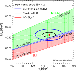
Figure 1: The present experimental accuracy for $m_{W}$ and $m_{t}$ after the experiments at LEP and Tevatron (large ellipse) and the expected accuracies at Tevatron + LHC (medium size ellipse) and LC + GigaZ (small ellipse). The upper and lower bands show the predictions of SM and MSSM, respectively, where the small intermediate band denotes the overlap between the predictions of SM and MSSM. From Ref. HeinemeyerPlot.

From this analysis we learn that a heavy particle can be probed when it appears in the virtual loops of the quantum corrections. As these loop effects influence some of the measurable observables, it may be possible to derive limits on the allowed mass range of this heavy particle. This is possible although the energy is not high enough to directly produce the heavy particle in experiment. The prize to be paid is, of course, high precision in experiment as well as in the theoretical calculation.

2.2 Higgs Boson Searches

For a complete verification of the SM and its electroweak symmetry breaking mechanism we have to find the Higgs boson. In the preceding section we have seen that consistency of the SM with the existing precision data requires $m_{h}<260$ GeV. Combining the final results from LEP2 of the four experiments ALEPH, DEPLPHI, L3 and OPAL a lower bound for the SM Higgs boson mass of $114.4$ GeV at $95\%$ confidence level arises.[3, 4] A considerable part of the allowed mass range for the Higgs boson is within the reach of Tevatron. A full coverage of this mass range will be provided by LHC and a future $e^{+}e^{-}$ linear collider or muon collider. The search for the Higgs boson, therefore, has high priority at all present and future colliders. In this section we will discuss the principle ideas of Higgs boson searches at the Tevatron, LHC and a future $e^{+}e^{-}$ linear collider.

The main production mechanisms at hadron colliders are gluon–gluon fusion, $WW$ or $ZZ$ fusion, associated production with $W$ or $Z$ and associated production with $t\bar{t}$ or $b\bar{b}$.[17] At the $p\bar{p}$ collider Tevatron with $\sqrt{s}=2$ TeV the most relevant production mechanism is the associated production with $W$ or $Z$ bosons, where a detectable rate of Higgs events is expected for $m_{h}=120$ GeV and an integrated luminosity $\int\mathcal{L}=2~{}\mathrm{fb}^{-1}$. For example, a clear signature is expected for the reaction[18]

$$p+\bar{p}\rightarrow W^{\pm}+h\rightarrow\ell^{\pm}+(q\bar{q})+p_{\mathit{T}\mathrm{miss}}$$ (11)

where $85\%$ of the $q\bar{q}$ pairs are $b\bar{b}$, and the $\nu_{\ell}$ from $W^{\pm}\rightarrow\ell^{\pm}\nu_{\ell},\ell=e,\mu$ is reconstructed from the missing transverse momentum $p_{\mathit{T}\mathrm{miss}}$. The $WW$ or $ZZ$ fusion cross sections are slightly smaller for $m_{h}\lesssim 150$ GeV. The cross sections for associated production with $t\bar{t}$ or $b\bar{b}$ are rather low.

The dominant production mechanism at the LHC with $\sqrt{s}=14$ TeV is gluon–gluon fusion with a cross section $\gtrsim 10~{}\mathrm{pb}$ for $m_{h}<260$ GeV. The cross section for $WW$ or $ZZ$ fusion is of the order of a few pb, whereas the cross sections for the associated productions with gauge bosons or $t\bar{t}$, $b\bar{b}$ may contribute for lower Higgs masses.

The search for the Higgs boson will also have a very high priority at a future linear collider.[6] The production of a SM Higgs boson in $e^{+}e^{-}$ annihilation can proceed via “Higgsstrahlung” $e^{+}e^{-}\to Zh$, $WW$ fusion $e^{+}e^{-}\to\nu_{e}\bar{\nu}_{e}h$, and $ZZ$ fusion $e^{+}e^{-}\to e^{+}e^{-}h$. At $\sqrt{s}=500$ GeV the Higgsstrahlung process dominates for $m_{h}\gtrsim 160$ GeV, whereas for $m_{H}\lesssim 160$ GeV the $WW$ fusion process gives the largest contribution. The higher $\sqrt{s}$ the more important is the $WW$ fusion process. The Feynman diagrams for the Higgsstrahlung and the $WW$ fusion processes are shown in Fig. 2. Only for $\sqrt{s}\gtrsim 800$ GeV the $ZZ$ fusion process can contribute about $\gtrsim 10\,\%$ of the total production rate. If $m_{h}\lesssim 260$ GeV as suggested by the electroweak precision data, an optimal choice for the c.m.s. energy is $\sqrt{s}\approx 350$ – $500$ GeV.

Figure 2: Feynman diagrams for the Higgsstrahlung and $WW$ fusion production mechanisms of SM Higgs bosons in $e^{+}e^{+}$ annihilation.

In conclusion one can say that there are some prospects of finding the Higgs boson at the Tevatron. The LHC will cover the full mass range up to $m_{h}\approx 1$ TeV. Precise determinations of all important Higgs boson couplings will be possible at a future $e^{+}e^{-}$ linear collider or muon collider.[6, 18]

3 Grand Unification

We can study the scale dependence of the three gauge coupling “constants” with the help of the renormalization group equations (RGE). If we evolve the strong, electromagnetic and weak coupling constants to higher energy scales, they become approximately equal at $M_{U}\approx 10^{14}$ GeV to $10^{16}$ GeV, the grand unification scale. This behaviour of the gauge coupling constants suggests that the SM is embedded into an underlying grand unified theory (GUT). If we assume that this GUT is also a gauge theory, its symmetry group has to be semi-simple and it has to contain $SU(3)\times SU(2)\times U(1)$ as a subgroup. The GUT gauge group is unbroken at energies higher than the GUT scale $M_{U}$, and is spontaneously broken to the SM gauge group at lower energies. The smallest semi-simple GUT group with rank 4 is $SU(5)$. Other possible choices are $SO(10)$, $E(6)$ etc. In this section we will shortly mention the basic features of $SU(5)$ and $SO(10)$ grand unification (for other examples see Refs. ross,moha,Mohapatra:1999vv).

In the $SU(5)$ GUT model the 15 helicity states of each family of quarks and leptons are put into the $\mathbf{\bar{5}}$ ($e_{L}$, $\nu_{eL}$, $d^{C}_{iL}$, $i=1,2,3$) and $\mathbf{10}$ ($e^{C}_{L}$, $u_{iL}$, $u^{C}_{iL}$, $d_{iL}$, $i=1,2,3$) representations. Here the right–handed states $f_{R}$ are written as the charge conjugate left–handed states $f^{C}_{L}$, and $i=1,2,3$ denotes the three colours of the quarks. Furthermore the $SU(5)$ GUT model contains 24 vector bosons corresponding to the 24 generators of the Lie group $SU(5)$, i.e. the gluons, the electroweak gauge bosons and 12 new coloured and charged gauge bosons called $X$ and $Y$ which are leptoquarks and diquarks. The spontaneous breaking of $SU(5)$ can be achieved in a two-step procedure. In a first step a $\mathbf{24}$ multiplet of scalar Higgs fields with masses $\mathcal{O}(M_{U})$ breaks $SU(5)$ to the SM group $SU(3)\times SU(2)\times U(1)$. In a second step the SM group is broken to $SU(3)\times U(1)$ by a $\mathbf{5}$ multiplet of Higgs fields with masses $\mathcal{O}(m_{Z})$.

The gauge bosons $X$ have couplings of the form $X\ell q$ with leptons and quarks and can therefore induce proton decay, for example, $p\rightarrow\pi^{0}e^{+}$. The mass of the vector bosons $X$ has to be of the order $m_{X}\approx M_{U}$. The order of magnitude for the proton lifetime can be estimated as $\tau_{p}^{-1}\approx\alpha_{U}^{2}m_{p}^{2}/m_{X}^{2}$, where $m_{p}$ is the proton mass. In the non-supersymmetric $SU(5)$ GUT model with $M_{U}\approx 10^{14}$ GeV one obtains $\tau_{p}\approx 10^{30}$ years, whereas the present experimental lower bound for the proton lifetime is $\tau_{p}>1.9\times 10^{33}$ years. In the supersymmetric $SU(5)$ GUT model the unification scale turns out to be $M_{U}\approx 10^{16}$ GeV. This leads to a larger value for the proton lifetime, which is in agreement with the experimental lower bound although the parameter space of the supersymmetric $SU(5)$ GUT is tightly constrained.[22]

The supersymmetric $SO(10)$ GUT model has a number of additional desirable features compared to $SU(5)$.[21, 23] For example, the 15 helicity states of quarks and leptons together with a SM gauge singlet right-handed neutrino state leading to nonzero neutrino masses are included in one $\mathbf{16}$ representation of $SO(10)$. Furthermore the $SO(10)$ GUT model can solve the SUSY CP and $R$-parity problems because it is left-right symmetric. There are many ways to break $SO(10)$ down to the SM, details can be found in Ref. Mohapatra:1999vv.

4 Supersymmetry

Supersymmetry (SUSY) is a new symmetry relating bosons and fermions. The particles combined in a SUSY multiplet have spins which differ by $\frac{1}{2}$. This is different from the symmetries of the SM or a GUT where all particles in a multiplet have the same spin (for an introduction to SUSY see e.g. Ref. wess).

SUSY is at present one of the most attractive and best studied extensions of the SM. The most important motivation for that is the fact that SUSY quantum field theories have in general better high–energy behaviour than non–SUSY ones. This is due to the cancellation of the divergent bosonic and fermionic contributions to the 1-loop radiative corrections. A particularly important example is the cancellation of the quadratic divergencies in the loop corrections to the Higgs mass. This cancellation mechanism provides one of the best ways we know to stabilize the mass of an elementary scalar Higgs field against radiative corrections and keep it “naturally” of the order $\mathcal{O}(m_{Z})$.

Practically all SUSY modifications of the SM are based on local $N=1$ SUSY. In the “minimal” SUSY extension of the SM a hypothetical SUSY partner is introduced for every known SM particle. The SUSY partners of the neutrinos, leptons, and quarks are called scalar neutrinos $\tilde{\nu}$, left and right scalar leptons $\tilde{\ell}_{L}$, $\tilde{\ell}_{R}$, and left and right scalar quarks $\tilde{q}_{L}$, $\tilde{q}_{R}$, respectively. They have spin $0$. The SUSY partners of the gauge vector bosons have spin $\frac{1}{2}$ and are called gauginos. The photino $\tilde{\gamma}$, $W^{\pm}$-ino $\tilde{W}^{\pm}$, $Z$-ino $\tilde{Z}$, and gluino $\tilde{g}$ are the partners of $\gamma$, $W^{\pm}$, $Z^{0}$, and the gluon, respectively. In the local version of SUSY the graviton gets a spin–$\frac{3}{2}$ SUSY partner, called gravitino. Furthermore, at least two isodoublets of Higgs fields $H_{i},i=1,2$, have to be introduced, together with their SUSY partners, the higgsinos $\tilde{H}_{i},i=1,2$, which have spin $\frac{1}{2}$. In this way the anomalies in the triangular loops cancel. The model obtained in this way is the Minimal Supersymmetric Standard Model (MSSM).[25] In the “next-to-minimal” SUSY extension of the SM (NMSSM) an additional Higgs singlet and the corresponding higgsino are introduced (see for example Ref. NMSSM and References therein).

The gauginos and higgsinos form quantum mechanically mixed states. The charged and neutral mass eigenstates are the charginos $\tilde{\chi}_{i}^{\pm}$, $i=1,2$, and neutralinos $\tilde{\chi}_{i}^{0}$, $i=1,\dots 4$, respectively. The left and right states of the scalar fermions are also mixed, with a mixing term proportional to the corresponding fermion mass. Therefore, the mass eigenstates of the first and second generation scalar fermions are to a good approximation the left and right states. However, there may be strong left–right mixing in the sector of the scalar top and bottom quarks and the scalar tau lepton.

If SUSY was an exact symmetry, then the masses of the SUSY partners would be the same as those of the corresponding SM particles. This is evidently not observed in nature, therefore, SUSY must be broken. Essentially, the idea is to break local SUSY spontaneously at a high energy scale.[27] The result is the global SUSY Lagrangian plus additional “soft SUSY–breaking terms”, which are mass terms for the SUSY partners, and additional trilinear coupling terms for the scalar fields.[19, 20, 25] Further assumptions are necessary to fix the additional soft–breaking parameters. For example, we can assume that at the GUT scale $M_{U}$ all scalar SUSY partners have the same mass $M_{0}$, all gauginos have a common mass $M_{1/2}$, and all trilinear couplings of the scalar fields have a common strength $A_{0}$. We obtain their values at the weak scale by evolving them with the RGEs from $Q=M_{U}$ to $Q\approx M_{Z}$.[28] The model obtained in this way is called constrained MSSM (CMSSM) or minimal supergravity-inspired model (mSUGRA). In Fig. 3 we show an example where we plot the gaugino mass parameters $M_{1}$, $M_{2}$, $M_{3}$ as a function of the scale $Q$.

Figure 3: Evolution of the gaugino mass parameters $M_{i}$ from low to high scales. From Ref. Allanach:2004ed.

Radiative electroweak symmetry breaking is a further attractive feature of SUSY. This can be achieved by exploiting the logarithmic scale dependence of the squares of the masses of the Higgs fields $H_{1}^{0}$ and $H_{2}^{0}$. Starting at the scale $Q=M_{U}$ with the mass values $M_{H_{1}}^{2}=M_{H_{2}}^{2}=M_{0}^{2}$ and evolving to lower energies, it turns out that $M_{H_{2}}^{2}$ can become negative at $Q\approx M_{Z}$. The reason is that $M_{H_{2}}^{2}$ gets large negative contributions from the top–quark loops. In this way spontaneous breaking of the electroweak symmetry is induced. $H_{1}^{0}$ and $H_{2}^{0}$ get vev’s $\langle H_{i}^{0}\rangle=\frac{1}{\sqrt{2}}v_{i},i=1,2$, and the vector bosons get masses $m_{W}^{2}=\frac{1}{4}g^{2}(v_{1}^{2}+v_{2}^{2})$ and $m_{Z}^{2}=\frac{1}{4}(g^{2}+g^{\prime 2})(v_{1}^{2}+v_{2}^{2})$. This mechanism works because the top–quark mass is much larger than the other quark masses (as one can show $m_{t}>60$ GeV must be fulfilled). Furthermore, the mass difference between the SM particles and their SUSY partners must be less than about 1 TeV.

The Higgs sector of the MSSM contains five Higgs bosons, the $CP$–even $h^{0}$ and $H^{0}$, the $CP$–odd $A^{0}$, and a pair of charged ones, $H^{\pm}$.[30] An important prediction of the MSSM is that the mass of the lighter $CP$–even state $h^{0}$ is always $m_{h^{0}}<m_{Z}$ at tree–level. There are large radiative corrections which change this prediction to $m_{h^{0}}\lesssim 140$ GeV.[31, 32] Comparing with the discussion in subsection 2.1 we see that this prediction for $m_{h^{0}}$ lies within the allowed range for the Higgs boson mass obtained in the analysis of the electroweak precision data. We note in passing that some SUSY parameters may be complex and induce CP-violating effects, for example, mixing between the CP-odd $A^{0}$ and the CP-even $h^{0}$ and $H^{0}$.[32, 33]

It turns out that the unification of the three gauge couplings works better in the MSSM than without SUSY.[28] We illustrate this in Fig. 4, where we plot the gauge couplings in the MSSM as a function of the energy scale. The evolution in the MSSM is different from that in the SM, because the RGEs of the MSSM contain also the contributions from the SUSY particles. In the MSSM the unification scale turns out to be of the order $M_{U}\approx 2\times 10^{16}$ GeV, provided the masses of the SUSY particles are not much larger than approximately $1$ TeV.

Figure 4: (a) Running of the inverse gauge couplings from low to high energies. (b) Expansion of the area around $Q=10^{16}$ GeV. The wide error bands are based on present data, and the spectrum of supersymmetric particles from LHC measurements within mSUGRA. The narrow bands demonstrate the improvement expected by future GigaZ analyses and the measurement of the complete spectrum at “LHC+LC”. From Ref. Allanach:2004ed.

The experimental search for SUSY particles has a high priority at present colliders and will become even more important at LHC and the future $e^{+}e^{-}$ linear collider ILC. In the discussion of the possible signatures one has to distinguish the two cases whether the multiplicative quantum number $R$-parity $R_{P}=(-1)^{3B+L-2S}$ is conserved or violated. SUSY particles have $R_{P}=-1$ and ordinary particles have $R_{P}=+1$. If $R_{P}$ is conserved, then there exists a lightest SUSY particle (LSP) which is stable. Cosmological arguments suggest that it is neutral and only weakly interacting. It is an excellent candidate for dark matter. We assume that the lightest neutralino $\tilde{\chi}_{1}^{0}$ is the LSP, which in the CMSSM holds in most of the parameter space. In experiment the LSP behaves like a neutrino and its energy and momentum are not observable. Therefore, in the $R_{P}$ conserving case the characteristic experimental signatures for SUSY particles are events with missing energy $E_{\mathrm{miss}}$ and missing momentum $p_{\mathrm{miss}}$.

In the $R_{P}$ violating case the SUSY Lagrangian contains additional terms which are allowed by SUSY and the gauge symmetry, but are lepton number violating and/or baryon number violating. Consequently, the LSP is not stable and decays into SM particles. Therefore, in the $R_{P}$ violating case the $E_{\mathrm{miss}}$ and $p_{\mathrm{miss}}$ signature is in general not applicable. However, due to the decay of the LSP there are more leptons and/or jets in the final state. At an $e^{+}e^{-}$ collider the main signature for $R_{P}$ violation is, therefore, an enhanced rate of multi-lepton and/or multi-jet final states. If the mean decay length of the LSP is too large and it decays outside the detector, then its energy and momentum remain invisible and the $E_{\mathrm{miss}}$ and $p_{\mathrm{miss}}$ signature is again applicable. If the LSP decays within the detector and the decay length is long enough, then displaced vertices may occur, which then provide a further important observable for $R_{P}$ violating SUSY. At a hadron collider the situation may be more involved. If the lepton number violating terms dominate over the baryon number violating ones, then the enhanced number of multi-lepton final states is again a good signature.

$R_{P}$ violating SUSY can also provide a viable framework for non-vanishing neutrino masses and a quantitative description of the present data on neutrino oscillations. This is a very attractive feature of $R_{P}$ violating SUSY, which in its bilinear formulation can be shortly described in the following way (for a review see Ref. Hirsch:2004he): As lepton number is not conserved, the neutrinos mix with the neutralinos and the charged leptons mix with the charginos, where the amount of mixing depends on the $R_{P}$ violating parameters. In bilinear $R_{P}$ violating SUSY one neutrino gets a non-vanishing mass already at tree level, while the other two neutrinos get their masses at 1-loop level. In this way “small” neutrino masses are obtained and the data on neutrino oscillations can be quantitatively described. After fixing the $R_{P}$ violating parameters by the solar and atmospheric neutrino data, the $R_{P}$ violating decay widths of the SUSY particles can be predicted. This means that the low energy phenomena in the neutrino sector are linked to the SUSY particle sector, which we expect to probe at high energy colliders.

At LEP no supersymmetric particles have been found.[35] This implies lower mass bounds which are $m_{\tilde{\chi}^{\pm}_{1}}>103.5$ GeV (for $m_{\tilde{\nu}_{e}}>300$ GeV), $m_{\tilde{e}}>99.9$ GeV, $m_{\tilde{\mu}}>94.9$ GeV, $m_{\tilde{\tau}}>86.6$ GeV, $m_{\tilde{t}}>95$ GeV and $m_{\tilde{b}}>94$ GeV. The limit on the mass of $\tilde{\chi}_{1}^{0}$ is model dependent. Within the CMSSM the non–observation of charginos and neutralinos excludes certain CMSSM parameter regions. From these follows the limit on the $\tilde{\chi}_{1}^{0}$ mass $m_{\tilde{\chi}_{1}^{0}}>50.3$ GeV. The non–observation of Higgs bosons leads to the mass limits $m_{h^{0}}>92.9$ GeV and $m_{A^{0}}>93.3$ GeV in the CP-conserving MSSM with real parameters. In the CP-violating MSSM with complex parameters no universal lower bound for the masses of the neutral Higgs bosons can be defined.[36]

At the Tevatron the strong interaction processes of gluino and squark production, $p\bar{p}\rightarrow\tilde{g}\tilde{g}$, $\tilde{g}\tilde{q}$, $\tilde{q}\bar{\tilde{q}}$, are the SUSY reactions with the highest cross sections. Gluinos and squarks may have cascade decays which start with $\tilde{g}\rightarrow q\bar{q}\tilde{\chi}_{i}^{0}$, $q\bar{q}^{\prime}\tilde{\chi}_{i}^{\pm}$, $\tilde{q}\rightarrow q\tilde{\chi}_{i}^{0}$, $\tilde{q}\rightarrow q^{\prime}\tilde{\chi}_{i}^{\pm}$, and continue until the LSP $\tilde{\chi}_{1}^{0}$ is reached. Suitable kinematical cuts are necessary to distinguish a possible signal from the huge SM background. The present gluino and squark mass limits are $m_{\tilde{g}}\gtrsim 400$ GeV, and $m_{\tilde{q}}\gtrsim 250$ GeV if $m_{\tilde{q}}\approx m_{\tilde{g}}$, $m_{\tilde{q}}\gtrsim 200$ GeV if $m_{\tilde{g}}\approx 500$ GeV whereas for $m_{\tilde{g}}\gtrsim 560$ GeV no limit on the squark mass can be obtained from measurements at Tevatron.[37] For $\tilde{t}_{1}$ and $\tilde{b}_{1}$ the mass limits are different: $m_{\tilde{t}_{1}}\gtrsim 115$ GeV provided $m_{\tilde{\chi}_{1}^{0}}\lesssim 50$ GeV and $m_{\tilde{b}_{1}}\gtrsim 140$ GeV provided $m_{\tilde{\chi}_{1}^{0}}\lesssim 70$ GeV, respectively.[35] Another interesting SUSY reaction which can be studied at the hadron colliders is $p\bar{p}\rightarrow\tilde{\chi}_{1}^{\pm}\tilde{\chi}_{2}^{0}$. It leads to the very clean signature $3\ell+p_{\mathrm{miss}}$, $\ell=e,\mu$.[38] The Tevatron mass limit for $\tilde{\chi}_{1}^{\pm}$, following from the non-observation of this reaction, is close to the LEP limit. At the upgraded Tevatron the expected SUSY mass reach will be $m_{\tilde{g}}\approx m_{\tilde{q}}\approx 390$ GeV, $m_{\tilde{t}_{1}}\approx 180$ GeV, $m_{\tilde{\chi}_{1}^{\pm}}\approx 250$ GeV, for an integrated luminosity of $2~{}\mathrm{fb}^{-1}$.

At LHC gluinos and squarks will be detectable up to masses of approximately $1-2$ TeV, as is illustrated in Fig. 5. The cascade decays of these particles will play an important role.[39] On the one hand they will give rise to characteristic signatures, for example the same–sign dilepton signature of gluinos. On the other hand, in the cascade decays the weakly interacting charginos and neutralinos will appear whose properties can also be studied. If weak–scale SUSY is not found at the Tevatron, then the LHC is the collider where it will be either discovered or definitely disproved.

The reach in the mSUGRA parameter space of an $e^{+}e^{-}$ linear collider with $\sqrt{s}=0.5$ to 1 TeV will be be somewhat smaller than that of the LHC (Fig. 5 (b)). However, due to the high luminosity and good energy resolution expected an $e^{+}e^{-}$ linear collider will be inevitable for precision measurements, especially in the neutralino and chargino sectors. This will enable us to determine very precisely the SUSY parameters and to reconstruct the underlying theory.[6, 28, 42] However, the signatures will be more complicated than those at LEP, because also the heavier SUSY particles will be produced which have cascade decays. This will lead to characteristic events with several leptons and/or jets, and missing energy and momentum.

Inspecting again Fig. 1 it can be seen that already the precision data obtained at the GigaZ mode of the linear collider (small ellipse) will presumably allow us to discriminate between the SM and the MSSM or another extension of the SM. The present experimental errors (large ellipse) do not allow to discriminate between the two models. In this figure the MSSM band is obtained by varying the SUSY parameters in the range allowed by the experimental and theoretical constraints. There is a small overlap of the SM and MSSM bands (small intermediate band) for a light Higgs boson ($m_{h}=113$ GeV) and a heavy SUSY spectrum.

Figure 5: (a) The reach of the LHC for various production channels of SUSY particles in the the mSUGRA model for $\tan\beta=30$, $A_{0}=0$ and $\mu>0$, assuming 100 fb^-1 of integrated luminosity. The shaded regions are excluded by theoretical and experimental constraints. From Ref. Baer:2003wx. (b) Reach of an $e^{+}e^{-}$ linear collider with $\sqrt{s}=0.5$ and 1 TeV in the mSUGRA model for $\tan\beta=30$, $A_{0}=0$ and $\mu>0$. For comparison the reach of the Tevatron assuming 10 fb^-1 of integrated luminosity (for isolated trileptons) and the reach of the LHC (in the “inclusive” $\not\!\!E_{T}$ channel) assuming 100 fb^-1 of integrated luminosity is shown. The dark shaded region is excluded by theoretical constraints. The gray shaded region shows points where the relic density $\Omega h^{2}<0.129$ as preferred by WMAP. The light shaded region is excluded by LEP2. From Ref. Baer:2003ru.

5 Extra dimensions

A solution to the hierarchy problem can in principle be obtained by formulating gravity in $4+\delta$ dimensions, where $\delta=1,2,3,\ldots$ are the so-called “extra” dimensions,[43, 44] which are assumed to be compactified with a radius $R$ (for a review see Ref. Rizzo:2004kr). In the model of Ref. add it is assumed that SM physics is restricted to the 4-dimensional brane, whereas gravity acts in the $4+\delta$ dimensional bulk. In 4-dimensional space-time the Planck mass is $M_{\mathrm{Pl}}=1.2\cdot 10^{19}$ GeV. In the $(4+\delta)$-dimensional space the corresponding Planck mass $M_{D}$ is given by $M_{D}^{2+\delta}=M_{\mathrm{Pl}}^{2}/R^{\delta}$. Assuming further that the compactification radius $R$ is many orders of magnitude larger than the Planck length, $R\gg M_{\mathrm{Pl}}^{-1}$, $R$ and $\delta$ may be adjusted such that $M_{D}\approx\mathcal{O}(1~{}\textrm{TeV})$. In this way the Planck scale is close to the electroweak scale and there is no hierarchy problem.

As a consequence of the compactification Kaluza-Klein towers of the gravitons can be excited. This leads to two possible signatures at an $e^{+}e^{-}$ linear collider. The first one is $e^{+}e^{-}\to\gamma/Z+G_{n}$ where $G_{n}$ means the graviton and its Kaluza-Klein excitations, which appear as missing energy in the detector. The main background to this process is $e^{+}e^{-}\to\nu\bar{\nu}\gamma$, which strongly depends on the $e^{-}$ beam polarisation. The second signature is due to graviton exchange in $e^{+}e^{-}\to f\bar{f}$, which leads to a modification of cross sections and asymmetries compared to the SM prediction.

References

-
[1]
There is an extensive literature on gauge field theories and the
Standard Model. We mention two books and refer also to the
literature cited therein:
O. Nachtmann, Elementary Particle Physics, Springer–Verlag
(1990);
M. E. Peskin and D. V. Schroeder, An Introduction to Quantum Field Theory, Addison-Wesley (1995). - [2] S. Petcov, lecture at the VII School on Non-Accelerator Astroparticle Physics, July 26 – August 6, 2004, Trieste, Italy.
- [3] G. Giacomelli, lecture at the VII School on Non-Accelerator Astroparticle Physics, July 26 – August 6, 2004, Trieste, Italy.
- [4] R. Barate et al. [The LEP Collaborations ALEPH, DELPHI, L3, OPAL and the LEP Electroweak Working Group], Phys. Lett. B 565 (2003) 61 [arXiv:hep-ex/0306033].
- [5] J. G. Branson, D. Denegri, I. Hinchliffe, F. Gianotti, F. E. Paige and P. Sphicas [ATLAS and CMS Collaborations], Eur. Phys. J. directC 4 (2002) N1.
-
[6]
E. Accomando et al. [ECFA/DESY LC Physics Working Group
Collaboration],
Phys. Rept. 299 (1998) 1
[arXiv:hep-ph/9705442];
T. Abe et al. [American Linear Collider Working Group Collaboration], in Proc. of the APS/DPF/DPB Summer Study on the Future of Particle Physics (Snowmass 2001) ed. N. Graf, arXiv:hep-ex/0106056;
J. A. Aguilar-Saavedra et al. [ECFA/DESY LC Physics Working Group Collaboration], arXiv:hep-ph/0106315;
K. Abe et al. [ACFA Linear Collider Working Group Collaboration], arXiv:hep-ph/0109166. - [7] W. Hollik et al., Acta Phys. Polon. B 35 (2004) 2533 and References therein.
- [8] S. Heinemeyer, W. Hollik and G. Weiglein, arXiv:hep-ph/0412214.
- [9] J. F. Gunion, H. E. Haber, G. L. Kane, and S. Dawson, The Higgs Hunter’s Guide, Addison-Wesley (1990).
-
[10]
S. Eidelman et al. [Particle Data Group Collaboration],
Phys. Lett. B 592 (2004) 1,
see
http://pdg.lbl.gov/. - [11] The LEP Collaborations ALEPH, DELPHI, L3, OPAL, the LEP Electroweak Working Group, the SLD Electroweak and Heavy Flavour Groups, arXiv:hep-ex/0312023.
- [12] F. Jegerlehner, arXiv:hep-ph/0312372.
- [13] M. J. G. Veltman, Nucl. Phys. B 123 (1977) 89.
- [14] G. Altarelli, arXiv:hep-ph/0406270.
-
[15]
G. Weiglein, talk at the
International Conference on Linear Colliders, LCWS 04,
April 19–22, 2004;
S. Heinemeyer and G. Weiglein, arXiv:hep-ph/0012364. -
[16]
The LEP Electroweak Working Group,
http://lepewwg.web.cern.ch/LEPEWWG/. - [17] A. Djouadi, Pramana 60 (2003) 215 [arXiv:hep-ph/0205248].
- [18] J. Gunion et al., Proc. of the 1996 DPF/DPB Summer Study on High–Energy Physics, Snowmass, Colorado, Vol. 2, p. 541, eds. D. G. Cassel, L. Trindle Gennari, R. H. Siemann.
- [19] G. G. Ross, Grand Unified Theories, Addison–Wesley (1985).
- [20] R. N. Mohapatra, Unification and Supersymmetry, Springer–Verlag (1986).
- [21] R. N. Mohapatra, arXiv:hep-ph/9911272.
- [22] B. Bajc, P. Fileviez Perez and G. Senjanovic, Phys. Rev. D 66 (2002) 075005 [arXiv:hep-ph/0204311].
- [23] H. Baer, M. Brhlik, M. A. Diaz, J. Ferrandis, P. Mercadante, P. Quintana and X. Tata, Phys. Rev. D 63 (2001) 015007 [arXiv:hep-ph/0005027].
-
[24]
J. Wess and J. Bagger, Supersymmetry and Supergravity, Princeton
University Press (1983);
D. Bailin and A. Love, Supersymmetric Gauge Field Theory and String Theory, IOP Publishing (1994). -
[25]
H. P. Nilles,
Phys. Rept. 110 (1984) 1;
H. E. Haber and G. L. Kane, Phys. Rept. 117 (1985) 75. -
[26]
F. Franke and H. Fraas,
Int. J. Mod. Phys. A 12 (1997) 479
[arXiv:hep-ph/9512366];
U. Ellwanger, J. F. Gunion and C. Hugonie, arXiv:hep-ph/0406215. - [27] R. Arnowitt, A. Chamseddine, and P. Nath, Applied N=1 Supergravity, World Scientific (1984).
- [28] G. A. Blair, W. Porod and P. M. Zerwas, Eur. Phys. J. C 27 (2003) 263 [arXiv:hep-ph/0210058].
- [29] B. C. Allanach et al., arXiv:hep-ph/0407067.
- [30] J. F. Gunion and H. E. Haber, Nucl. Phys. B 272 (1986) 1 [Erratum-ibid. B 402 (1993) 567].
- [31] M. Carena and H. E. Haber, Prog. Part. Nucl. Phys. 50 (2003) 63 [arXiv:hep-ph/0208209].
- [32] S. Heinemeyer, arXiv:hep-ph/0407244.
- [33] M. Carena, J. R. Ellis, A. Pilaftsis and C. E. M. Wagner, Nucl. Phys. B 586 (2000) 92 [arXiv:hep-ph/0003180].
- [34] M. Hirsch and J. W. F. Valle, New J. Phys. 6 (2004) 76 [arXiv:hep-ph/0405015].
-
[35]
The LEP SUSY Working Group, ALEPH, DELPHI, L3 and OPAL Collaborations,
http://lepsusy.web.cern.ch/lepsusy/Welcome.html. -
[36]
The LEP Working Group for Higgs Boson Searches,
ALEPH, DELPHI, L3 and OPAL Collaborations,
http://lephiggs.web.cern.ch/LEPHIGGS/www/Welcome.html. - [37] A. Meyer, talk at the 32nd International Conference on High Energy Physics, ICHEP’04, August 16–22, 2004, Beijing, China.
- [38] H. Baer and X. Tata, Phys. Rev. D 47 (1993) 2739.
-
[39]
H. Baer, C. h. Chen, F. Paige and X. Tata,
Phys. Rev. D 49 (1994) 3283
[arXiv:hep-ph/9311248];
Phys. Rev. D 50 (1994) 4508
[arXiv:hep-ph/9404212];
D. Denegri, W. Majerotto and L. Rurua, Phys. Rev. D 58 (1998) 095010 [arXiv:hep-ph/9711357];
A. Bartl et al. Proc. of the 1996 DPF/DPB Summer Study on High–Energy Physics, Snowmass, Colorado, Vol. 2, p. 693, eds. D. G. Cassel, L. Trindle Gennari, R. H. Siemann. - [40] H. Baer, C. Balazs, A. Belyaev, T. Krupovnickas and X. Tata, JHEP 0306 (2003) 054 [arXiv:hep-ph/0304303].
- [41] H. Baer, A. Belyaev, T. Krupovnickas and X. Tata, JHEP 0402 (2004) 007 [arXiv:hep-ph/0311351].
- [42] G. Weiglein et al. [The LHC / LC Study Group], arXiv:hep-ph/0410364.
-
[43]
N. Arkani-Hamed, S. Dimopoulos and G. R. Dvali,
Phys. Lett. B 429 (1998) 263
[arXiv:hep-ph/9803315];
Phys. Rev. D 59 (1999) 086004
[arXiv:hep-ph/9807344];
I. Antoniadis, N. Arkani-Hamed, S. Dimopoulos and G. R. Dvali, Phys. Lett. B 436 (1998) 257 [arXiv:hep-ph/9804398]. - [44] L. Randall and R. Sundrum, Phys. Rev. Lett. 83 (1999) 3370 [arXiv:hep-ph/9905221].
- [45] T. G. Rizzo, arXiv:hep-ph/0409309 and References therein.