Conference Summary

Department of Physics
University of California, San Diego
La Jolla, CA 92093-0319, USA

1 Flavor Physics Deep Questions

Having heard of the tremendous progress seen in the last year in the field of flavor physics and CP violation, I would like to invite the audience to contemplate some of the questions we are ultimately trying to answer, and to ponder how much progress has been made towards answering them. Some of these deep questions are

• Why are there several generations of quarks and leptons? Are there precisely three? Is there some underlying structure that explains the presence of generations? Are the generations really identical except for the mass, or is there some basic distinction between them?

• Is there a fundamental explanation to the hierarchy of masses? Is there are a relation between quark and lepton masses, or between quarks/leptons of different generations?

• What gives rise to the texture of mixings between generations? Is this related to the masses of quarks and leptons?

• Is flavor physics tied to Electro-Weak symmetry breaking?

• What is the origin of the observed CP violation? Is the CP violation in the mixings (of quarks and leptons) enough to accommodate baryogenesis or leptogenesis? Else, what is the nature of additional CP violation?

• Is there a relation between quarks and leptons? Are the patterns of masses, mixings and CP violation related?

The lack of evidence for quark and lepton substructure makes difficult addressing these questions. It is worth revisiting our current approach. Seemingly the community of flavor/CP physicists has concentrated their efforts on measuring with ever increasing precision the parameters of the standard model that pertain to flavor physics and CP violation, e.g., masses and mixing parameters.

Why is this the right strategy? In the absence of indications of underlying structure, we are left with the task of looking for ever subtler deviations from the predictions of the standard model. We ought to be testing specific theories of flavor, like supersymmetric extensions of the standard model, extended technicolor, leptoquarks, overlapping branes, CKM textures, etc. But detailed quantitative tests of these mathematical constructs have never resulted in confirmation of a theory. What is worse, rarely is a theory ruled out (a famous counterexample is the super-weak theory of CP violation). Some of these theoretical constructs are not very specific in their predictions and are rightfully largely ignored. And most models are only marginally predictive: they share the disturbing feature that they can be made as unobservable as needed by assuming that their effects become significant only at ultra-high energies.

Since theories of flavor fail to indicate useful directions in which we should test them, we simply press for higher precision and for tests of consistency of the standard model of flavor: the dominant task in the field is to both predict and measure at the highest precision possible. Ever more precise results are parametrized in the CKM standard model, a theory which does not address flavor, but rather accommodates it.

It comes as little surprise that most of the talks at this conference focus on precise determination of parameters and tests of consistency. While answering the “deep questions” remains the primary goal, the daunting task of determining the (possibly changing) standard is interesting enough in its own right. We should succeed at describing the universe in detail, if not in explaining why the universe is that way!

Little thought has been given to the scenario in which the standard CKM model successfully accommodates every result regardless of precision attained. It may then be that there is no underlying quantum field theory model of flavor. Instead, the answer to some of the “deep questions” may require thinking outside the box, and may require invoking some often maligned ideas such as the anthropic principle and quantum cosmology.

This write-up of my summary talk, as the talk itself, leaves out many interesting subjects presented at the conference. I apologize to those participants whose hard work I could not include here. This is entirely due to space and time limitations. I have freely quoted from the talks, and have therefore limited my citations to other entries in these proceedings, with a few exceptions that correspond to instances in which I had to consult or quote additional external sources.

2 The flavor of leptons: Neutrino masses and mixing

It is now firmly established that neutrinos mix and therefore $m_{\nu}\neq 0$. A summary of evidence for neutrino masses and mixings is shown in Fig. 1. The oscillation probability, $P(\nu_{1}\rightarrow\nu_{2})=\sin^{2}2\theta\sin^{2}(1.27\Delta m^{2}L/E)$, depends both on the mixing angle $\theta$ and the mass difference $\Delta m$. The atmospheric neutrino data ($\nu_{\mu}\rightarrow\nu_{X}$) is confirmed and gives $\Delta m^{2}\sim 2\times 10^{-3}\text{eV}^{2}$ with near-maximal mixing. Solar neutrino oscillations ($\nu_{e}\rightarrow\nu_{X}$) are also confirmed, with non-maximal mixing and $\Delta m^{2}\sim 8\times 10^{-5}\text{eV}^{2}$. The LSND reports small angle oscillations in $\overline{\nu}_{\mu}\rightarrow\overline{\nu}_{e}$ with small mixing angle and $\Delta m^{2}\sim 0.1$–$10\text{~{}eV}^{2}$. The MiniBoonNE experiment will be in a position to confirm or refute this observation. Since neutrinos are neutral their mass may be either Dirac or Majorana.

A Dirac mass would make the lepton sector similar to the quark sector. It requires new fields beyond those in the standard model, namely, right handed neutrinos. This raises some interesting questions. How many right handed neutrinos are there? How many of them are active and how many inactive? In this scenario a lepton sector version of the CKM matrix arises naturally, the Pontecorvo-Maki-Nakagawa-Sakata matrix (PMNS), and one can ask if this is in any way related to the CKM matrix and whether the masses are related to those of quarks. Total lepton number is conserved, just like baryon number is conserved in the quark sector. And just like for quarks, individual flavor number is broken. The PMNS automatically accommodates CP violating phases which give rise to the possibility of CP violation for leptogenesis and raises the question of measuring lepto-CP violation in the lab.

Figure 1: Summary of neutrino mass and mixing evidence[1].

A Majorana mass would be even more exciting. It is a new phenomenon and raises new questions. For example, are there new scalar fields with vacuum expectation values responsible for these masses? Lepton number is violated (the mass term has $|\Delta L|=2$). The Majorana neutrino is by necessity active ($\Delta I_{w}=1$). The mass could arise from a triplet Higgs or from the see-saw mechanism through a dimension five term in the Lagrangian. The latter, being non-renormalizable, could be interpreted as the result of new short distance interactions. In addition there could be sterile neutrinos with a bare mass (or with a singlet Higgs giving mass) which could mix with the active ones.

The observations indicate an interesting pattern of masses. Ignoring the LSND observations one has two disparate mass differences indicating that two neutrinos are almost degenerate, on the scale of the mass difference with the third. However, since there is no measurement of the individual mass of any neutrino it is not known whether the almost degenerate pair is lighter (“normal hierarchy”) or heavier (“inverted hierarchy”) than the third neutrino. The normal hierarchy is akin that observed in the quark sector, and it will be interesting to see if there is a connection between sectors. For a Majorana mass the inverted hierarchy may lead to observable neutrino-less double beta decay, but for the normal hierarchy the rate is unobservably much smaller.

The LSND observation, if confirmed, requires the addition of a new neutrino, since three disparate mass differences require four distinct mass eigenstates. Measurements of the width of the $Z$-vector boson set to three the number of active neutrinos with mass less than $m_{Z}/2$. Hence any additional light neutrinos must be sterile. Some constraints on these already exist from present experiments. Pure $\nu_{\mu}-\nu_{s}$ mixing is excluded for atmospheric neutrinos (SK, MACRO), while pure $\nu_{e}-\nu_{s}$ mixing is excluded for solar neutrinos (SK, SNO). The mass patterns can be of two types, either “2+2”, in which two pairs of neutrinos are degenerate on the scale of the large (LSND) mass difference, or “3+1”, in which a much heavier neutrino is added to either of the hierarchies of the previous paragraph.

The future bodes well and busy for neutrino physics. Many experiments are continuing and many more proposed. MiniBoonNE will either confirm or refute the LSND findings. Long baseline experiments will narrow the $\nu_{\mu}-\nu_{\tau}$ parameter space, search for $\nu_{\mu}\rightarrow\nu_{e}$ and improve significantly the precision of oscillation parameters (K2K-II, MINOS, CNGS, NOvA, T2K). Proposed dedicated reactor experiments (Angra dos Reis, Braidwood, Chooz-II, Diablo Canyon, Daya Bay, Kashiwazaki, Krasnoyarsk) will measure $\theta_{13}$ with higher sensitivity and may establish it does not vanish[2]. Proposed double beta decay experiments may demonstrate the Majorana nature of neutrino mass (CUORE, GENIUS, Majorana, super-NEMO, MOON,EXO). Searches for CP violation in the lepton sector could culminate in a complete theory of leptogenesis[3]. There is reason to be optimistic!

3 The CKM Matrix

3.1 Status

Elements of the CKM matrix,

$$V_{\rm CKM}=\begin{pmatrix}V_{ud}&V_{us}&V_{ub}\\ V_{cd}&V_{cs}&V_{cb}\\ V_{td}&V_{ts}&V_{tb}\end{pmatrix}$$ (1)

are determined with widely varying precision. While unitarity can be used to significantly constrain individual elements of the matrix, a determination that does not assume unitarity tests this feature. Let’s briefly review our knowledge of individual elements, without assuming unitarity.

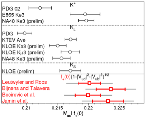
Figure 2: Current status of experiments in the $V_{us}$ determination[4].

The best determined element is $V_{ub}$. It is obtained from nuclear beta decay and the error is only 0.2%.

Next best known is the Cabibbo angle, or $V_{us}$, which the PDG claims to be known at the 1% level. It is determined from $K\ell 3$ decays. However, there are inconsistencies between the most recent (E685, NA48, KTeV, KLOE) measurements of decay rates and the summary of older experiments in the PDG. This is just as well because there are also inconsistencies between the quoted values and unitarity of the CKM. A tremendous effort was undertaken to resolve these inconsistencies[4]. The current experimental situation is summarized in Fig. 2, which shows that the new rates are all consistently higher than the PDG values. The decay rate is given in terms of a form factor $f_{+}$ (parametrizing the matrix element of the hadronic current) and the CKM element, so to extract $V_{us}$ and test unitarity of the CKM matrix one needs theory to predict the form factor. The last row in Fig. 2 shows the rate as predicted by CKM-unitarity using different theory calculations of the form factor. The degree of consistency depends on which calculation is adopted. Just as with experiment, there is a renewed effort to re-analyze the theory of these decays. Two new calculations of form factors have appeared, one using chiral perturbation theory extending the classic calculation of Leutwyler and Roos, and one using quenched lattice QCD. While the calculations differ only by about 2%, the deviation is of practical importance, particularly when the PDG claims a precision of 1% in $V_{us}$. It is tempting to favor the lattice calculation over the chiral perturbation theory one, partly because it agrees with the older Leutwyler-Roos and partly because the lattice is supposed to be unadulterated QCD. But, reader beware, quenched lattice calculations are non-systematic approximations. Moreover, the deviation between theoretical calculations is as large as one could expect it to be! Recall that the form factor is protected by the Ademollo-Gatto theorem:

$$f_{+}(0)=1+0\cdot\epsilon+\mathcal{O}(\epsilon^{2})$$ (2)

where $\epsilon\sim m_{s}/{\mathchar 28931\relax_{\rm QCD}}\sim 1/3$ is the dimensionless symmetry breaking parameter ($\epsilon\sim m_{K}^{2}/\mathchar 28931\relax_{\chi}^{2}\sim 1/4$ in chiral perturbation theory). If the quenching error is of typical magnitude, $\sim 20$%, then the error in $f_{+}(0)$ ought to be $20\text{\%}\times\epsilon^{2}\sim 2\text{\%}$.

It is rather surprising that $V_{cd}$ and $V_{cs}$ are poorly known. Charm production in neutrino scattering ($\nu+d\rightarrow c+X$) gives a 5% determination of $V_{cd}$, while $W^{+}$ decays to charm give a 10% determination of $V_{cs}$. These are two elements where progress would be welcome. It is hard to believe that these could not benefit from the advances in understanding of inclusive semileptonic decays of heavy mesons, which have yielded a $1-2\text{\%}$ measurement of $V_{cb}$.

Currently, the errors in the determination of $V_{cb}$ and $V_{ub}$ are about 1% and 10%, respectively. These will be discussed in some detail below, since they are the focus of a large effort in the flavor community and there has been much progress recently.

The last row of the CKM is known the least. $V_{tb}$ is determined at the 20% level from top quark decay, but $V_{td}$ and $V_{ts}$ can only be accessed indirectly, through electroweak loops as in, for example, $B^{0}-\overline{B}{}^{0}$ mixing and radiative $B$ decays.

4 Over-constraining the unitarity triangle

Unitarity of the CKM matrix and the freedom to redefine fields result in only four independent parameters needed to parametrize the matrix. The Wolfenstein parametrization,

$$V_{\rm CKM}=\begin{pmatrix}V_{ud}&V_{us}&V_{ub}\\ V_{cd}&V_{cs}&V_{cb}\\ V_{td}&V_{ts}&V_{tb}\end{pmatrix}\approx\begin{pmatrix}1-{\textstyle{\frac{1}{2}}}\lambda^{2}&\lambda&A\lambda^{3}(\overline{\rho}-i\overline{\eta})\\ -\lambda(1+iA^{2}\lambda^{4}\overline{\eta}&1-{\textstyle{\frac{1}{2}}}\lambda^{2}&A\lambda^{2}\\ A\lambda^{3}(1-\overline{\rho}-i\overline{\eta})&-A\lambda^{2}(1+i\lambda^{2}\overline{\eta})&1\end{pmatrix}+\mathcal{O}(\lambda^{6})$$ (3)

shows the four parameters explicitly and is most frequently used. Joining the points 0, 1 and $\overline{\rho}+i\overline{\eta}$ in the complex plane yields a unitarity triangle. The sides have length 1, $\sqrt{\overline{\rho}^{2}+\overline{\eta}^{2}}=|V_{ub}|/|V_{us}V_{cb}|$ and $\sqrt{(1-\overline{\rho})^{2}+\overline{\eta}^{2}}=|V_{td}|/|V_{us}V_{cb}|$. The triangle is determined, up to discreet ambiguities, by these lengths or, alternatively, by two of the three vertex angles, defined in the figure to the right. If the CKM picture of flavor and CP physics is correct, the same triangle should be inferred from decay rates as from CP asymmetries.

Figure 3: Babar fit to moments of the $B\rightarrow X_{c}\ell\nu_{\ell}$ spectrum[5].

4.1 Sides

4.1.1 $|V_{cb}|$ from inclusive semileptonic decays

In order to calculate the rate $d\Gamma(B\rightarrow X_{c}\ell\nu_{\ell})$ theorists use an expansion in powers of ${\mathchar 28931\relax_{\rm QCD}}/m_{b}$. The latest analyses retain terms up to and including order $({\mathchar 28931\relax_{\rm QCD}}/m_{b})^{3}$, incurring in an error $\sim({\mathchar 28931\relax_{\rm QCD}}/m_{b})^{4}\sim(0.1)^{4}$. The expansion introduces unknown non-perturbative parameters. These can be determined by measuring the semileptonic spectrum precisely.

To this effect experiment measures, and theory predicts, moments of the the decay spectrum. Commonly used are lepton energy moments,

$$\langle E^{n}_{\ell}\rangle_{E_{\text{cut}}}\equiv\frac{R_{n}({E_{\text{cut}}},0)}{R_{0}({E_{\text{cut}}},0)}\quad\text{where}\quad R_{n}({E_{\text{cut}}},M)\equiv\int_{E_{\text{cut}}}\!\!\!(E_{\ell}-M)^{n}\frac{{\rm d}\Gamma}{{\rm d}E_{\ell}}\,{\rm d}E_{\ell}\,,$$ (4)

and hadronic mass moments

$$\langle m_{X}^{2n}\rangle_{E_{\text{cut}}}\equiv\frac{\int_{E_{\text{cut}}}\!(m_{X}^{2})^{n}\frac{{\rm d}\Gamma}{{\rm d}m^{2}_{X}}\,{\rm d}m^{2}_{X}}{\int_{E_{\text{cut}}}\!\frac{{\rm d}\Gamma}{{\rm d}m^{2}_{X}}\,{\rm d}m^{2}_{X}}\,.$$ (5)

where $m_{X}^{2}\equiv(p_{B}-p_{\ell}-p_{\nu})^{2}=(p_{B}-q)^{2}$. Note that the moments are defined with a lepton energy cut. While this cut is an experimental necessity, measuring moments as a function of the cut allows for a stringent test of the theory and a better determination of parameters. Also included in the analysis are photon energy moments in $d\Gamma(B\rightarrow X_{s}\gamma)$, which depend on the same unknown hadronic parameters as their semileptonic counterparts.

BaBar has performed a fit[5] using the theoretical analysis of Gambino and collaborators and of Bataglia and Uraltsev. The results, in Fig. 3, show very nice agreement between theory and experiment, and the resulting value for the CKM angle is $|V_{cb}|=(41.4\pm 0.4_{\text{exp}}\pm 0.4_{\text{HQE}}\pm 0.6_{\text{theory}})\times 10^{-3}$. In addition, Bauer and collaborators have performed a global fit to data from BaBar, Belle, CDF, CLEO and DELPHI, with comparable results, as explained elsewhere in these proceedings[6].

Figure 4: Summary of $|V_{cb}|$ and $|V_{ub}|$ determinations.

4.1.2 $|V_{cb}|$ from exclusive semileptonic decays

The differential decay rate

$$\frac{{\rm d}\Gamma(B\rightarrow D^{*}\ell\overline{\nu})}{{\rm d}w}=\frac{G_{F}^{2}m_{B}^{5}}{48\pi^{3}}\,r_{*}^{3}\,(1-r_{*})^{2}\,\sqrt{w^{2}-1}\,(w+1)^{2}\left[1+\frac{4w}{1+w}\frac{1-2wr_{*}+r_{*}^{2}}{(1-r_{*})^{2}}\right]|V_{cb}|^{2}\,{{\cal F}_{*}{}^{2}(w)}$$

is parametrized in terms of ${\cal F}_{*}$, a combination of form factors of the $V-A$ charged current. Here $w\equiv p_{B}\cdot p_{D}^{*}/M_{B}M_{D}^{*}$, and $r^{*}=M_{D}^{*}/M_{B}$. At lowest order in HQET ${\cal F}_{*}(1)=1$, and Luke’s Theorem insures the corrections are small, ${\cal F}_{*}(1)-\eta_{\text{QCD}}=\mathcal{O}({\mathchar 28931\relax_{\rm QCD}}/m_{c})^{2}$, where $\eta_{\text{QCD}}$ is a known short distance QCD correction. Since the rate vanishes at $w=1$, to determine $|V_{cb}|$ an extrapolation of the data to $w=1$ must be made. This is aided by theory, since analyticity and unitarity tightly constrain the functional form of ${{\cal F}_{*}(w)}$.

The precision in the determination of $|V_{cb}|$ from exclusive decays is limited by a 4% uncertainty in ${\cal F}_{*}(1)$. While only marginally competitive with the inclusive determination, it provides an independent test of theory.

4.1.3 $|V_{ub}|$ from inclusive semileptonic decays

The rate for charm-less semileptonic $B$ decays is much smaller than for charm-full decays. Hence experimental kinematic cuts that exclude the charm-full decays are needed. One may cut in the hadronic mass, $m_{X}^{2}=(P_{B}-p_{\ell}-p_{\nu})^{2}$, the lepton mass $q^{2}=(p_{\ell}+p_{\nu})^{2}$ or the charged lepton energy $E_{\ell}$. In all three cases the rate is significantly limited, with the cut on $q^{2}$ being the most limiting. The theory of inclusive charm-less $B$ decays is, in principle, the same as for charm-full decays. But in practice the necessary cuts complicate matters. If the cut is not too stringent so the decay is not dominated by a few resonances but rather by low invariant mass jets then the theory can still be organized through an OPE but now an infinite number of “leading twist” terms contribute equally. This infinite sum can be parametrized by a shape function which encodes our ignorance of strong interactions. The challenge is to make model independent predictions.

At leading order in a $1/m_{b}$ expansion the shape function in $B\rightarrow X_{u}\ell\nu$ is the same that appears in the rate for $B\rightarrow X_{s}\gamma$. In principle then one can determine the shape function from $B\rightarrow X_{s}\gamma$ and use it in the determination of $|V_{ub}|$ from $B\rightarrow X_{u}\ell\nu$. In practice, however, the $1/m_{b}$ corrections, which spoil the equality of the shape function in the two processes, can be large. The naive guess ${\mathchar 28931\relax_{\rm QCD}}/m_{b}\sim 10\text{\%}$ is not far off from detailed estimates.

Both Belle and BaBar have determined $|V_{ub}|$ by this method. I quote here the result but warn the audience that the theoretical uncertainties from $1/m_{b}$ corrections have not been properly accounted for resulting in a (probably large) underestimate of theoretical error:

$$\text{Belle:}\quad|V_{ub}| =(5.54\pm 0.42\pm 0.55\pm 0.42\pm 0.27)\times 10^{-3}$$

$$\text{BaBar:}\quad|V_{ub}| =(5.18\pm 0.41\pm 0.40\pm 0.23\pm 0.27)\times 10^{-3}$$

Here the errors are statistical, experimental, fit and OPE (theory), respectively. Fig. 4 shows the HFAG compilation of results for the determination of $|V_{ub}|$[8].

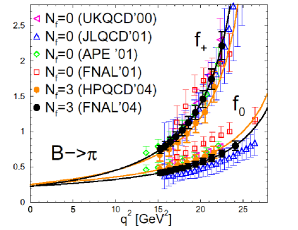
Figure 5: Form factors for $B\rightarrow\pi\ell\nu$ computed by simulations of lattice QCD[9].

4.1.4 $|V_{ub}|$ from exclusive semileptonic decays

As in the case of inclusives the situation for $|V_{ub}|$ is worse than for $|V_{cb}|$. The problem is that HQET does not fix normalization at zero recoil as it does in $B\rightarrow D^{(*)}\ell\nu$. For $B\rightarrow\pi\ell\nu$ two form factors determine the decay amplitude: The determination of $|V_{ub}|$ from exclusive decays requires a priori knowledge of the form factor $f_{+}$ for $B\rightarrow\pi$, defined through

$$\langle\pi(p_{\pi})|\overline{b}\gamma_{\mu}q|B(p_{B})\rangle=\left((p_{B}+p_{\pi})_{\mu}-\frac{m_{B}^{2}-m_{\pi}^{2}}{q^{2}}q_{\mu}\right){F_{+}(q^{2})}+\frac{m_{B}^{2}-m_{\pi}^{2}}{q^{2}}q_{\mu}{F_{0}(q^{2})}\,,$$ (6)

where $q\equiv p_{B}-p_{\pi}$. Analyticity and unitarity do constrain the functional form, which helps, e.g., to interpolate lattice results. A compilation of lattice results is shown in Fig. 5. One can use this to determine $|V_{ub}|$, but the errors are large. Belle finds, from $B\rightarrow\pi\ell\nu$ restricted to $q^{2}>16\text{GeV}^{2}$, $|V_{ub}|=(3.87\pm 0.70\pm 0.22^{+0.85}_{-0.51})\times 10^{-3}$ and $|V_{ub}|=(4.73\pm 0.85\pm 0.27^{+0.74}_{-0.50})\times 10^{-3}$ using lattice results from FNAL’04 and HPQCD, respectively. The theory errors, $\sim\pm 20$%, are not expected to be significantly reduced soon. There has also been some effort to understand the precision with which $|V_{td}|$ can be determined from $B\rightarrow\rho\gamma$ decays[6].

New ideas are needed to reduce the error on $|V_{ub}|$ from exclusive decays to the sub-10% level, hopefully to a few percent. One recent proposal is to use double ratios to eliminate hadronic uncertainties. While the method is promising a detail theoretical error analysis is missing, as are experimental feasibility studies[6].

4.2 Angles

The direct route to measuring angles is through CP violation in interference between decay and mixing in the decay of a neutral $B$ meson to a CP eigenstate $f_{\text{CP}}$. The asymmetry

$$a_{f}=\frac{\Gamma[\overline{B}{}^{0}(t)\rightarrow f]-\Gamma[B^{0}(t)\rightarrow f]}{\Gamma[\overline{B}{}^{0}(t)\rightarrow f]+\Gamma[B^{0}(t)\rightarrow f]}=S_{f}\sin(\Delta mt)-C_{f}\cos(\Delta mt)$$ (7)

is theoretically clean if the final state is a CP eigenstate and only one weak phase contributes (or is dominant), in which case

$$a_{f_{\text{CP}}}=\text{Im}\;\lambda_{f_{\text{CP}}}\sin(\Delta mt).$$ (8)

Here $\lambda_{f_{\text{CP}}}=(q/p)\overline{\mathcal{A}}_{f_{\text{CP}}}/\mathcal{A}_{f_{\text{CP}}}$ depends on the weak mixing angles through the $B^{0}-\overline{B}{}^{0}$ mixing parameters $p$ and $q$, and through the ratio of amplitudes for $\overline{B}{}^{0}$ and $B^{0}$ decays, $\overline{\mathcal{A}}_{f_{\text{CP}}}$ and $\mathcal{A}_{f_{\text{CP}}}$, to the common final state $f_{\text{CP}}$. The coefficient of $\cos(\Delta mt)$ is also often denoted by $A_{f}=-C_{f}$, but this notation may be confusing given the proliferation of A’s (in Wolfenstein’s parametrization, to denote asymmetries and to denote amplitudes).

Figure 6: Standard model fit as reported by CKMfitter[11] (above) and in the BaBar book, circa 1998 (below). The figures are drawn to different scale.

4.2.1 $\sin(2\phi_{1})$ from $b\rightarrow c\overline{c}s$

Great precision has been achieved by both Belle and BaBar in the determination of $\sin(2\phi_{1})$ from $B$ decays to charmonium plus $K^{0}$[10]:

$$\text{BaBar:}\quad\sin(2\phi_{1}) =+0.722\pm 040\pm 023$$

$$\text{Belle:}\quad\sin(2\phi_{1}) =+0.728\pm 056\pm 033$$

We can finally over-constrain the unitarity triangle. Figure 6 shows CKMfitter standard model fit including this $S_{\psi K}$ data. The obvious first remark is that the standard model works remarkably well. Clearly we want to keep piling on observables to this global fit. It should be noted that the determination of $\cos(2\phi_{1})$, while interesting, adds little to this program. It is also quite clear, from the precision achieved, that further progress requires we concentrate on clean observables, for which model dependence does not cloud the issue of interpretation of experimental results.

It is interesting to ponder on what the best next direction may be. From Fig. 6 it is clear that pinning down the apex of the unitarity triangle would be best achieved by measuring the length of the side opposite the origin, that is, $|1-(\overline{\rho}+i\overline{\eta})|$, since this is orthogonal to the direction fixed by $\phi_{1}$. This is tested by $B^{0}-\overline{B}{}^{0}$ oscillations and by $b\rightarrow d$ decays, like $B\rightarrow\rho\gamma$ (for which a branching fraction upper limit of $1.2\times 10^{-6}$ has been established). Alternatively, one may measure $\sin(2\phi_{3})$ with precision.

But if testing consistency of the picture is what we are after, measuring the length $|\overline{\rho}+i\overline{\eta}|$ is best, since this is largely parallel to the direction fixed by $\phi_{1}$. Hence advances in measuring $|V_{ub}|$ are of paramount importance.

It is nice to see how much progress has been made. Figure 6, reproduced from the BaBar book (circa 1998), shows the status in the determination of the unitarity triangle six years ago, allowing a much wider region for the apex of the triangle.

4.2.2 $\sin(2\phi_{1})$ from $b\rightarrow c\overline{c}d$, $b\rightarrow q\overline{q}s$

$\sin(2\phi_{1})$ can also be determined, albeit less cleanly, from $b\rightarrow c\overline{c}d$, $b\rightarrow q\overline{q}s$ decays. Some extensions of the standard model allow for significant deviations in $-\eta_{f}S_{f}$ from $\sin(2\phi_{1})$ in individual processes (here $\eta_{f}$ is the CP parity of the final state $f$). Unfortunately, theoretical predictions for these decays are less clean, with an uncertainty in $-\eta_{f}S_{f}-\sin(2\phi_{1})$ guessed at 0.1 – 0.2.

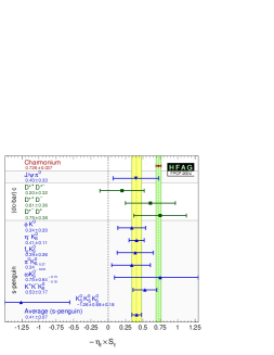
Figure 7: Compilation of results for $-\eta_{f}S_{f}$ from different modes[8]. The $K^{0}_{s}K^{0}_{s}K^{0}_{s}$ was new at this conference.

Figure 7 shows a compilation of results for several processes. The result for $f=K^{0}_{s}K^{0}_{s}K^{0}_{s}$ was first presented at this conference[16, 17] and shows a central value that dramatically deviates from expectation albeit with large errors. While no single observation significantly deviates from expectations, there is a disturbing (welcome, perhaps?) trend in the $b\rightarrow q\overline{q}s$ decays. Averaging results,

$$S_{\psi K}-\langle-\eta_{f}S_{f(b\rightarrow s)}\rangle =0.30\pm 0.08$$

$$S_{\psi K}-\langle-\eta_{f}S_{\eta^{\prime}K_{s},\phi K_{s}}\rangle =0.33\pm 0.11$$

These are $3.5\sigma$ and $3.1\sigma$ effects respectively. It will be interesting to see how this measurements evolve in the future and whether theory provides a more certain prediction of the expected deviation.

These deviations, if they persist, could be accommodated by non-extravagant extensions of the standard model. This would hardly be the case if the deviations were much larger. Take for example SUSY models[12, 13, 14, 15]. While LR insertions are severely constrained by $B\rightarrow X_{s}\gamma$, LL/RR penguins can give significant contributions. These, however, are beginning to be constrained by $\text{Br}(B\rightarrow X_{s}\ell\ell)=(4.5\pm 1.0)\times 10^{-6}$. This is another story whose development is worth watching!

4.2.3 Measurement of $\phi_{2}$ and $\phi_{3}$

Another remarkable recent development is the measurement of the other two unitarity angles, $\phi_{2}$ and $\phi_{3}$[16, 18, 19, 20, 17, 21].

Three methods have been used for the measurement of $\sin(2\phi_{2})$:

• $B\rightarrow\pi\pi$. This requires an isospin analysis. The branching fraction into $\pi^{0}\pi^{0}$ and $C_{\pi^{0}\pi^{0}}$ have been measured making the analysis viable. The results from Belle and BaBar for both $\sin(2\phi_{2}^{\text{eff}})$ and $C_{\pi^{+}\pi^{-}}$ differ significantly but the errors are still large (for a discussion see [23]).

• $B\rightarrow\rho\rho$ benefits from the small neutral branching fraction, $\text{Br}(\rho^{0}\rho^{0})/\text{Br}(\rho^{+}\rho^{-})<0.04$$(90\text{\%~{}CL})$. This implies that $\phi_{2}-\phi_{2}^{\text{eff}}$ is small.

• $B\rightarrow\rho\pi$ Dalitz plot. A clean determination requires a pentagon analysis which needs the branching fractions and CP asymmetries for the $\rho^{+}\pi^{-}$, $\rho^{0}\pi^{0}$ and $\rho^{-}\pi^{0}$ modes. Alternatively, $SU(3)$ flavor symmetry and factorization of the weak decay amplitude assumptions are used.

From the combined $\pi\pi$, $\rho\rho$ and $\rho\pi$ analysis, $\phi_{2}=(100\begin{smallmatrix}+12\\ -11\end{smallmatrix})^{\circ}$. This compares rather well with the CKM indirect constraint fit, $\phi_{2}=(98\pm 16)^{\circ}$.

$\sin(2\phi_{3})$ is determined from the interference between $B^{-}\rightarrow D^{0}K^{-}$ and $B^{-}\rightarrow\overline{D}{}^{0}K^{-}$, achieved with a final state common to $D^{0}$ and $\overline{D}{}^{0}$. A difficulty here is that the CP asymmetry is suppressed when the $D^{0}$ and $\overline{D}{}^{0}$ decay amplitudes to a particular final state differ vastly. Both $D^{0}$ and $\overline{D}{}^{0}$ have Cabibbo allowed decays to $K^{0}_{s}\pi^{+}\pi^{-}$, and the best present determination of $\sin(2\phi_{3})$ is from that analysis,

$$\text{Belle:}\quad\phi_{3} =(68\begin{smallmatrix}+14\\ -15\end{smallmatrix}\pm 13\pm 11)^{\circ}~{},$$

$$\text{BaBar:}\quad\gamma =(88\pm 41\pm 19\pm 10)^{\circ}~{},$$

where the errors are statistical, systematic and from model dependence. The much larger error quoted by BaBar is due to the large correlation in the error in $\gamma$ and the value of $r_{B}\equiv A(B^{-}\rightarrow\overline{D}{}^{0}K^{-})/A(B^{-}\rightarrow D^{0}K^{-})$, which is measured by Belle, $r_{B}=0.26\begin{smallmatrix}+0.11\\ -0.15\end{smallmatrix}\pm 0.03\pm 0.04$, while BaBar only obtains an upper bound $r_{B}<0.18~{}(\text{90\%~{}CL})$.

4.2.4 Direct CP violation: The last nail on the superweak coffin!

The superweak theory has all sources of CP violation in $\Delta B=2$ or $\Delta S=2$ interactions. Direct CP violation in decays of $B$ mesons proceed via $\Delta B=1$ interactions only, so a positive signal rules out the superweak theory. However, the interpretation of a signal does not immediately translate into a measurement of CKM phases. The CP asymmetry from two interfering amplitudes,

$$A_{CP}=\frac{2\sin(\varphi_{1}-\varphi_{2})\sin(\delta_{1}-\delta_{2})}{|A_{1}/A_{2}|+|A_{2}/A_{1}|+\cos(\varphi_{1}-\varphi_{2})\cos(\delta_{1}-\delta_{2})}$$ (9)

depends on unknown strong interaction phases $\delta_{i}$ and amplitudes $A_{i}$, in addition to the sought after weak phases $\varphi_{i}$. The combined analysis of Belle and BaBar gives $A_{CP}(B^{0}\rightarrow K^{+}\pi^{-})=-0.114\pm 0.020$, which is $5.7\sigma$ away from zero[22]. Interestingly, it is also found that $A_{CP}(B^{+}\rightarrow K^{+}\pi^{0})=-0.049\pm 0.040$, which, although compatible with zero, is $3.6\sigma$ away from $A_{CP}(B^{0}\rightarrow K^{+}\pi^{-})$ indicating that color-allowed tree amplitudes do not dominate color-suppressed trees (plus electroweak penguins).

5 Summary of the Summary

We have seen an evolution in flavor physics since the discovery of $D$ and $B$ mesons from a science which established new important qualitative facts, such as the long lifetime of $B$ mesons and the near diagonal structure of the CKM matrix, to what is now a precision science. At the same time we are witnessing the start of what promises to be a similar story in the lepton sector: the PMNS matrix is imprecisely known, much like CKM was 20 years ago. Both camps are tooling up for a next round of precision improvement and the future seems bright[24, 25, 26].

Have we seen a break with the standard paradigm? Certainly the positive result for neutrino masses requires some new physics beyond the standard model, be it new right handed fields or new interactions. And perhaps the hints of anomalies in $b\rightarrow s$ decays are an indication of surprises to come. Important steps toward answering the deep questions!

References

- [1] Eric Prebys, Status of MiniBooNE, talk at ICHEP2004
- [2] Takashi Kobayashi, these proceedings, pp. LABEL:KobayashiStart–LABEL:KobayashiEnd
- [3] Sin Kyu Kang, these proceedings, pp. LABEL:KangStart–LABEL:KangEnd
- [4] Sasha Glazov, these proceedings, pp. LABEL:GlazovStart–LABEL:GlazovEnd
- [5] Elisabetta Barberio, these proceedings, pp. LABEL:BarberioStart–LABEL:BarberioEnd
- [6] Benjamin Grinstein, these proceedings, pp.LABEL:GrinsteinStart–LABEL:GrinsteinEnd
- [7] P. F. Harrison and H. R. Quinn, “The BaBar physics book: Physics at an asymmetric B factory,” SLAC-R-0504
- [8] http://www.slac.stanford.edu/xorg/hfag/semi/summer04/summer04.shtml
- [9] Masataka Okamoto, these proceedings, pp. LABEL:OkamotoStart–LABEL:OkamotoEnd
- [10] Karim Trabelsi, these proceedings, pp. LABEL:TrabelsiStart–LABEL:TrabelsiEnd
- [11] http://www.slac.stanford.edu/xorg/ckmfitter
- [12] Tadashi Yoshikawa, these proceedings, pp.LABEL:YoshikawaStart–LABEL:YoshikawaEnd
- [13] Youngjoon Kwon, these proceedings, pp.LABEL:KwonStart–LABEL:KwonEnd
- [14] Pyungwon Ko, these proceedings, pp.LABEL:KoStart–LABEL:KoEnd
- [15] Alex Lenz, these proceedings pp. LABEL:LenzStart–LABEL:LenzEnd
- [16] Timothy Gershon, these proceedings, pp.LABEL:GershonStart–LABEL:GershonEnd
- [17] Masashi Hazumi, these proceedings, pp.LABEL:HazumiStart–LABEL:HazumiEnd
- [18] Adrian Bevan, these proceedings, pp.LABEL:BevanStart–LABEL:BevanEnd
- [19] Phil Clark, these proceedings, pp.LABEL:ClarkStart–LABEL:ClarkEnd
- [20] Justin Albert, these proceedings, pp.LABEL:AlbertStart–LABEL:AlbertEnd
- [21] Jure Zupan, these proceedings, pp.LABEL:ZupanStart–LABEL:ZupanEnd
- [22] Giacomo Graziani, these proceedings, pp.LABEL:GrazianiStart–LABEL:GrazianiEnd
- [23] A. Ichiro Sanda, these proceedings, pp.LABEL:SandaStart–LABEL:SandaEnd
- [24] Toru Iijima, these proceedings, pp.LABEL:IjimaStart–LABEL:IjimaEnd
- [25] Stephanie Menzemer, these proceedings, pp.LABEL:MenzemerStart–LABEL:MenzemerEnd
- [26] Peter Dornan, these proceedings, pp.LABEL:DornanStart–LABEL:DornanEnd