CKM Sides: Theory

Department of Physics
University of California, San Diego
La Jolla, CA 92093-0319, USA

We review the theory of the determination of the CKM elements $|V_{cb}|$ and $|V_{ub}|$. Particular attention is paid to the determination of $|V_{cb}|$ through inclusive semileptonic $B$ decays to charm using a moment analysis, since this has shown most progress recently. A precise method for the determination of $|V_{ub}|$ via exclusive decays is described.

1 Introduction

The Wolfenstein parametrization of the CKM matrix,

$$V_{\rm CKM}=\begin{pmatrix}V_{ud}&V_{us}&V_{ub}\\ V_{cd}&V_{cs}&V_{cb}\\ V_{td}&V_{ts}&V_{tb}\end{pmatrix}\approx\begin{pmatrix}1-{\textstyle{\frac{1}{2}}}\lambda^{2}&\lambda&A\lambda^{3}(\overline{\rho}-i\overline{\eta})\\ -\lambda(1+iA^{2}\lambda^{4}\overline{\eta}&1-{\textstyle{\frac{1}{2}}}\lambda^{2}&A\lambda^{2}\\ A\lambda^{3}(1-\overline{\rho}-i\overline{\eta})&-A\lambda^{2}(1+i\lambda^{2}\overline{\eta})&1\end{pmatrix}+\mathcal{O}(\lambda^{6})$$ (1)

shows explicitly that it is determined by four parameters. $K\ell 3$ decays determine $\lambda$ to 1% accuracy[1]. The other three parameters are the subject of this talk. As we will see, $|V_{cb}|=A\lambda^{2}$ is now determined to nearly 1% accuracy from $B\rightarrow X_{c}\ell\nu_{\ell}$. The magnitude of the remaining complex parameter, $\overline{\rho}-i\overline{\eta}=V_{ub}/(V_{us}V_{cb})$, is fixed from $B\rightarrow X_{u}\ell\nu_{\ell}$, but is known far less accurately.

Joining the points 0, 1 and $\overline{\rho}+i\overline{\eta}$ in the complex plane yields a unitarity triangle. The sides have length 1, $\sqrt{\overline{\rho}^{2}+\overline{\eta}^{2}}=|V_{ub}|/|V_{us}V_{cb}|$ and $\sqrt{(1-\overline{\rho})^{2}+\overline{\eta}^{2}}=|V_{td}|/|V_{us}V_{cb}|$. To determine the triangle one needs not just the magnitude but also the phase of $\overline{\rho}-i\overline{\eta}$. Alternatively, the length of the third side determines the triangle, up to a two-fold ambiguity. This third side can be obtained from $b\rightarrow d\gamma$ decays (eg, $B\rightarrow\rho\gamma$) or from the $B^{0}-\overline{B^{0}}$ mixing parameter $\Delta M_{d}$. In the standard model, both of these processes are dominated by a virtual top quark exchange and depend directly on $V^{\phantom{*}}_{td}V^{*}_{tb}$. The theory of these processes belongs in a different session in this conference[2, 3].

The bulk of the talk is devoted to the determination of $|V_{cb}|$ from inclusive decays $B\rightarrow X_{c}\ell\nu_{\ell}$, since here is where we have seen tremendous progress in the last year. Next we briefly revisit $|V_{cb}|$ from exclusive decays, $B\rightarrow D^{*}\ell\nu_{\ell}$ and $B\rightarrow D\ell\nu_{\ell}$. We then turn to $|V_{ub}|$ and mirroring the discussion above we first present its determination from inclusive decays, $B\rightarrow X_{u}\ell\nu_{\ell}$. This is followed by a review of the extraction of $|V_{ub}|$ from exclusives $B\rightarrow\pi(\rho)\ell\nu_{\ell}$. The limitted precission in the determination of $|V_{ub}|$ afforded by the standard methods calls for innovation in this area. We describe a new method that uses a combination of radiative and semileptonic $B$ and $D$ decays.

2 $|V_{cb}|$ from Inclusive decays $B\rightarrow X_{c}\ell\nu_{\ell}$

In QCD the differential width for $B\rightarrow X_{c}\ell\nu_{\ell}$ is a function of $|V_{cb}|$, the strong coupling $\alpha_{s}$ and the quark masses $m_{b}$ and $m_{c}$. Only the dependence on $|V_{cb}|$ is trivial:

$$\frac{d\Gamma(B\rightarrow X_{c}\ell\nu_{\ell})}{dx\,dy}={|V_{cb}|^{2}}f(x,y;m_{b,c},\alpha_{s}),$$ (2)

where $x,y$ are kinematic variables. Even if we could compute the function $f$ from first principles, we would still need as input precise values of the three parameters, $m_{b}$, $m_{c}$ and $\alpha_{s}$. While $\alpha_{s}$ is accurately known[4], the quark masses are not. For a determination of $V_{cb}$ one can use the measurement of the doubly differential decay rate to fit also the value of the masses.

Now, $V_{cb}$ enters only the overall normalization, while $m_{b}$ and $m_{c}$ determine the “shape” (i.e., the functional form) of the decay distribution. So one can isolate the determination of the masses by fitting to shape parameters, that is, various moments of the distribution. In all cases the moments are defined with a charged lepton energy cut, an experimental necessity turned into a theoretical tool. From the charged lepton integrals with an energy cut

$$R_{n}({E_{\text{cut}}},M)\equiv\int_{E_{\text{cut}}}\!\!\!(E_{\ell}-M)^{n}\frac{{\rm d}\Gamma}{{\rm d}E_{\ell}}\,{\rm d}E_{\ell}\,,$$ (3)

define moments

$$\langle E^{n}_{\ell}\rangle_{E_{\text{cut}}}\equiv\frac{R_{n}({E_{\text{cut}}},0)}{R_{0}({E_{\text{cut}}},0)}\,.$$ (4)

Central moments are also defined:

$$\langle(E_{\ell}-\langle E_{\ell}\rangle_{E_{\text{cut}}})^{n}\rangle_{E_{\text{cut}}}=\frac{R_{n}({E_{\text{cut}}},\langle E_{\ell}\rangle_{E_{\text{cut}}})}{R_{0}({E_{\text{cut}}},0)}\,.$$ (5)

Also useful are moments of the hadron invariant mass, $m_{X}^{2}\equiv(p_{B}-p_{\ell}-p_{\nu})^{2}=(p_{B}-q)^{2}$, defined by

$$\langle m_{X}^{2n}\rangle_{E_{\text{cut}}}\equiv\frac{\int_{E_{\text{cut}}}\!(m_{X}^{2})^{n}\frac{{\rm d}\Gamma}{{\rm d}m^{2}_{X}}\,{\rm d}m^{2}_{X}}{\int_{E_{\text{cut}}}\!\frac{{\rm d}\Gamma}{{\rm d}m^{2}_{X}}\,{\rm d}m^{2}_{X}}\,.$$ (6)

Central moments $\langle(m_{X}^{2}-{\overline{m}}^{2}_{D})^{n}\rangle$, about ${\overline{m}}^{2}_{D}\equiv\left[({m_{D}+3m_{D^{*}}})/4\right]^{2}$ are also frequently considered. Somewhat orthogonal information can be garnered from moments of the $B\rightarrow X_{s}\gamma$ spectrum, which depend on $m_{b}$ and $\alpha_{s}$, and only very weakly on $m_{c}$. They are defined for the spectrum of the photon energy in the $B$ rest frame, $E_{\gamma}$:

$$\langle E^{n}_{\gamma}\rangle\equiv\frac{\int_{E_{\text{cut}}}\!(E_{\gamma})^{n}\frac{{\rm d}\Gamma}{{\rm d}E_{\gamma}}\,{\rm d}E_{\gamma}}{\int_{E_{\text{cut}}}\!\frac{{\rm d}\Gamma}{{\rm d}E_{\gamma}}\,{\rm d}E_{\gamma}}$$ (7)

The variance, $\langle E_{\gamma}^{2}\rangle-\langle E_{\gamma}\rangle^{2}$, is often used, but higher moments are not, because they are very sensitive to the boost of the $B$ meson and to details of shape function.

2.1 Heavy Quark/Mass Expansion

At present we don’t know how to perform the calculation described above. Instead a systematic approximation to QCD is made by expanding in inverse powers of the heavy mass, $m_{b}$, and performing an operator product expansion[5]. The price we pay is that new dimensionful parameters are introduced. At $n$-th order in the expansion the new parameters are roughly of size $({\mathchar 28931\relax_{\rm QCD}})^{n}$, giving rise to an expansion in powers of $({\mathchar 28931\relax_{\rm QCD}}/m_{b})$. These new parameters account for our ignorance of non-perturbative dynamics in QCD.

There are two approaches to the expansion in the literature:

• The HQET/OPE, in which amplitudes are given in terms of mass independent heavy meson states. If one chooses to treat the $D^{(*)}$-meson as heavy then this approach involves an expansion in $1/m_{c}$ (in addition to $1/m_{b}$). The advantage is that $m_{c}$ can be fixed in terms of $m_{b}$ using the accurately determined $M_{D}-M_{B}$.

• The HME, or Heavy Mass Expansion, in which heavy meson states are not expanded (in neither $m_{c}$ nor $m_{b}$). No $1/m_{c}$ expansion is necessary. However, $m_{c}$ is a parameter determined from the fit.

Three groups have performed a moment analysis. The groups of M. Battaglia et al[6] and of Gambino and Uraltsev[7] use the HME, while C. Bauer et al[8] consider and compare both expansions. In all cases the expansion is up to (and including) terms of $\mathcal{O}({\mathchar 28931\relax_{\rm QCD}})^{3}$, and known perturbative corrections are included. More on this below.

2.2 Parameter Counting

It may come as a surprise that the number of parameters introduced by the two approaches is the same. The naive guess that the HQET/OPE with a $1/m_{c}$ expansion ought to introduce more parameters because it expands in $1/m_{c}$ too is incorrect. The additional expansion gives new information, for example, that to leading order the $B$ and $D$ meson states form heavy flavor symmetry doublets.

Altogether, there are six parameters (in addition to $\alpha_{s}$) that enter the moment analysis in either approach. With a $1/m_{c}$ expansion $m_{c}$ is fixed using $M_{B}-M_{D}$, and the parameters $\lambda_{2}\sim({\mathchar 28931\relax_{\rm QCD}})^{2}$ and $\rho_{2}\sim({\mathchar 28931\relax_{\rm QCD}})^{3}$ are fixed from $M_{B^{*}}-M_{B}$ and $M_{D^{*}}-M_{D}$. One is left with $m_{b}$, $\lambda_{1}\sim({\mathchar 28931\relax_{\rm QCD}})^{2}$, and four parameters of order $({\mathchar 28931\relax_{\rm QCD}})^{3}$, namely $\rho_{1}$ and three linear combinations of four time ordered products, $\mathcal{T}_{1-4}$. Now one has the issue of accuracy of expanding in $1/m_{c}$. The OPE is an expansion in $1/m_{b}$. It is only the computation of $m_{c}$ in terms of meson masses that requires a $1/m_{c}$ expansion. Since this is done to $\mathcal{O}({\mathchar 28931\relax_{\rm QCD}}/m_{c})^{3}$, the fractional error in $m_{c}$ is $\mathcal{O}({\mathchar 28931\relax_{\rm QCD}}/m_{c})^{4}$. But $m_{c}$ first enters the rate at $\mathcal{O}(m_{c}/m_{b})^{2}$, so the error introduced is $\mathcal{O}(\mathchar 28931\relax^{4}_{\text{QCD}}/m_{c}^{2}m_{b}^{2})$.

If the states are not expanded in $1/m$ (so no $1/m_{c}$ expansion is performed) then no time ordered products appear. However, $m_{c}$, $\lambda_{2}$ and $\rho_{2}$ cannot be solved in terms of physical meson masses, and they come in as parameters. Comparing with the counting above, the three combinations of time order products are replaced here by the three parameters $m_{c}$, $\lambda_{2}$ and $\rho_{2}$. Strictly speaking the parameters should be distinguished from the ones above and denoted by different symbols since in the HME the non-perturbative parameters have implicit dependence on the heavy quark mass. Bauer et al suggest that the fit to moments may be better behaved when the $1/m_{c}$ expansion is performed, since more of the parameters are of higher order in ${\mathchar 28931\relax_{\rm QCD}}$.

In either approach one needs to properly define quark masses. A good definition of the quark mass will give better convergence of the perturbatively calculable (in $\alpha_{s}$) Wilson coefficients of the OPE. Many definitions are available[9]. Threshold mass definitions, like the 1S and PS, give better convergence than the pole, $\overline{\text{MS}}$ or kinetic mass schemes. Battaglia et al and Gambino and Uraltsev use the kinetic mass scheme, while Bauer et al use all and compare. This latter group points out a problem with the kinetic mass. Since this scheme requires a rather low hard cut-off $\mu$, when there are two heavy quark masses, $m_{b}$ and $m_{c}$ one introduces two distinct hard cut-offs, $\mu_{b}$ and $\mu_{c}$. While it is customary to use $\mu_{b}=\mu_{c}$, there is nothing in principle which requires one to use equal cut-offs for the two masses. Bauer et al consider the effect of changing $\mu_{b,c}$ so that $\mu_{b}\neq\mu_{c}$, and find rather large variations in the determination of $|V_{cb}|$. The effect is due, presumably, to the next-order corrections in $\alpha_{s}(\mu_{b,c})$, which are rather large given that $\mu_{b,c}$ must be taken to be of the order of the fairly low scale $\sim 1$ GeV.

2.3 Fit results

The BaBar Collaboration has performed a fit to the moments calculated by Gambino and Uraltsev. The electron energy moments are computed to order $\beta_{0}\alpha_{s}^{2}$, $\alpha_{s}({\mathchar 28931\relax_{\rm QCD}})^{2}$ and $({\mathchar 28931\relax_{\rm QCD}})^{3}$, while the hadronic mass moments are computed to order $\alpha_{s}$, $\alpha_{s}({\mathchar 28931\relax_{\rm QCD}})^{2}$ and $({\mathchar 28931\relax_{\rm QCD}})^{3}$. To account for the missing order $\beta_{0}\alpha_{s}^{2}$ effects, the analysis uses a different value of $\alpha_{s}$ for the hadronic mass moments than for the lepton energy moments. This educated guess is somewhat ad hoc and introduces an unknown uncertainty. The result of the fit is presented in this conference elsewhere[10]. The fit includes non-integral moments of $m^{2}_{X}$, which are theoretically less well behaved and have larger uncertainties.

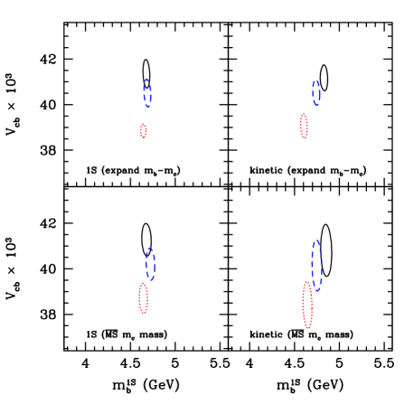
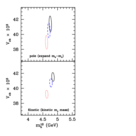
Figure 1: Convergence in $\alpha_{s}$ of the fit, in different schemes. The dotted (red) dashed (blue) and solid (black) ellipses denote the result of the fit when retaining terms of order $\alpha_{s}^{0}$, $\alpha_{s}$ and $\beta_{0}\alpha_{s}^{2}$, respectively.

The group of Bauer et al performs a global fit using data on semileptonic and radiative decays from the BABAR, BELLE, CDF, CLEO, DELPHI collaborations. They compare the two approaches, expanding or not in $m_{c}$, and the different mass schemes. Fig. 1 shows the convergence in $\alpha_{s}$ of the computation in different schemes. The dotted (red) dashed (blue) and solid (black) ellipses denote the result of the fit when retaining terms of order $\alpha_{s}^{0}$, $\alpha_{s}$ and $\beta_{0}\alpha_{s}^{2}$, respectively.

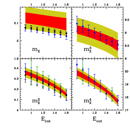
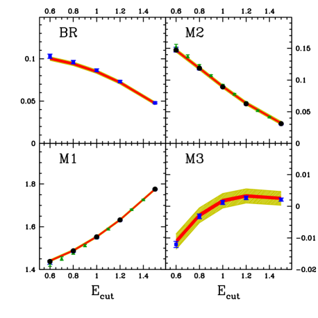
Figure 2: Fit of moments as a function of ${E_{\text{cut}}}$. The data points are from BABAR (squares), CLEO (triangles) and BELLE (circles).

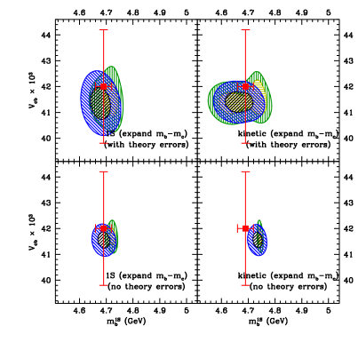
Figure 3: Result of fit for $|V_{cb}|$ and $m_{b}$. The lower graphs do not include theory errors and can be used to see the present theoretical limit of the extraction of parameters. The ellipses denote regions of $\Delta\chi^{2}=1$ (black and yellow), $\Delta\chi^{2}=4$ (blue and green). For the ellipses in black and blue the parameters of order $({\mathchar 28931\relax_{\rm QCD}})^{3}$ are restricted to vary within $\pm(500~{}\text{MeV})^{3}$, while no such restriction is used in the fit shown in yellow/green. The red cross shows the current PDG value of $|V_{cb}|$ and the 1S $m_{b}$ determined from a fit to bottomonium[11].

Figure 2 shows the result of the fit, for several moments as a function of ${E_{\text{cut}}}$. The data points are superimposed: square (blue), triangles (green) and filled circles (black) are from BABAR, CLEO and BELLE, respectively. The half integer hadronic moments are shown, but not used in the fit for $|V_{cb}|$. The shaded region indicates the theory error, which has been estimated from the size of the highest order retained in the double expansion in $\alpha_{s}$ and ${\mathchar 28931\relax_{\rm QCD}}/m_{b}$. The fit shown here is for the HQET/OPE approach (with $1/m_{c}$ expansion) in the 1S mass scheme. The graphs labeled BR and M1 show the branching fraction and the first lepton energy moment, while M2 and M3 show the second and third lepton energy central moments. The remarkable agreement between theory and experiment indicates that the expansion is working very well and, in particular, that local duality works extremely well for these decays. The result of the fit for $|V_{cb}|$ and $m_{b}$ is shown in Fig. 3. It is quite remarkable that the fitted value of $m_{b}$ is comparable to that obtained from masses of bottomonium and with comparable precision[11].

3 $|V_{cb}|$ from Exclusives: $B\rightarrow D^{*}\ell\nu_{\ell}$ and $B\rightarrow D\ell\nu_{\ell}$

The rates are given by the HQET-inspired parametrizations

$$\frac{{\rm d}\Gamma(B\rightarrow D^{*}\ell\overline{\nu})}{{\rm d}w} = \frac{G_{F}^{2}m_{B}^{5}}{48\pi^{3}}\,r_{*}^{3}\,(1-r_{*})^{2}\,\sqrt{w^{2}-1}\,(w+1)^{2}$$

$$\times\left[1+\frac{4w}{1+w}\frac{1-2wr_{*}+r_{*}^{2}}{(1-r_{*})^{2}}\right]|V_{cb}|^{2}\,{{\cal F}_{*}{}^{2}(w)}$$

$$\frac{{\rm d}\Gamma(B\rightarrow D\ell\overline{\nu})}{{\rm d}w} = \frac{G_{F}^{2}m_{B}^{5}}{48\pi^{3}}\,r^{3}\,(1+r)^{2}\,(w^{2}-1)^{3/2}\,|V_{cb}|^{2}\,{{\cal F}^{2}(w)}$$

in terms of ${\cal F}$ and ${\cal F}_{*}$, which are simply combination of form factors of $V-A$ charged currents. Here $w\equiv p_{B}\cdot p_{D}^{(*)}/M_{B}M_{D}^{(*)}$, and $r^{(*)}=M_{D}^{(*)}/M_{B}$. At lowest order in HQET ${{\cal F}(1)}={{\cal F}_{*}(1)}=1$, and Luke’s Theorem insures the corrections are small, ${\cal F}_{*}(1)-1=\mathcal{O}({\mathchar 28931\relax_{\rm QCD}}/m_{c})^{2}$.

In order to determine $|V_{cb}|$ we need an accurate theory of ${\cal F}_{*}(1)$, a measurement of the rate as a function of $w$ and an extrapolation of this measurement to $w=1$. Analyticity and unitarity tightly constrain the functional form of ${{\cal F}_{*}(w)}$[12]. Taylor expanding about $w=1$,

$${\cal F}_{*}(w)={\cal F}_{*}(1)[1+\rho^{2}(w-1)+c(w-1)^{2}+\ldots]$$ (8)

the unitarity constraint gives a relation between the slope, $\rho^{2}$, and curvature, $c$[13]. Sum rules give lower bounds on these parameters[14], but the bounds are not experimentally significant. It is interesting to note that at leading order in HQET the slope and curvature parameters are equal for ${\cal F}(w)$ and ${\cal F}_{*}(w)$. Corrections have been estimated, $\rho_{{\cal F}}^{2}-\rho_{{\cal F}_{*}}^{2}\simeq 0.19$, to be compared with the experimental fit, $\rho_{{\cal F}}^{2}-\rho_{{\cal F}_{*}}^{2}\simeq-0.22\pm 0.20$[17]. A more precise determination of the slopes and curvatures would help (and may tax) the theoretical understanding of sub-leading form factors in HQET.

The main limitation in determining $|V_{cb}|$ comes from theoretical uncertainties in ${\cal F}_{*}(1)-1$. The situation has not changed since the BaBar book was published, ${\cal F}_{*}(1)=0.91\pm 0.04$[15]. The current lattice determination has comparable errors, ${\cal F}_{*}(1)=0.913\begin{smallmatrix}+0.024\\ -0.017\end{smallmatrix}\begin{smallmatrix}+0.017\\ -0.030\end{smallmatrix}$[16]. For a comparison of the determinations of $|V_{cb}|$ from inclusive and exclusive decays see Ref. [10] in these proceedings.

4 $|V_{ub}|$ from inclusive $B\rightarrow X_{u}\ell\nu_{\ell}$

The theory of inclusive $b\rightarrow u\ell\nu$ processes is the same as in $b\rightarrow c\ell\nu$. However, a straightforward application of theory is not possible at the moment since experimentally the full spectrum is not available. The problem is that the signal is swamped by $B\rightarrow X_{c}\ell\nu_{\ell}$. The experimental solution: impose kinematic cuts to suppress the $b\rightarrow c$ background. By imposing either, $m_{X}<m_{D}$, $q^{2}>(m_{B}-m_{D})^{2}$ or $E_{\ell}>(m_{B}^{2}-m_{D}^{2})/2m_{B}$ one restricts the measurement to events which are not kinematically accessible to $b\rightarrow c$ decays. However, the experimental solution is largely incompatible with theory[20]. The endpoint spectra in $B\rightarrow X_{u}\ell\nu_{\ell}$ is given in terms of a non-perturbative “shape function,” $f(x)$. One approach is to measure $f(x)$ in $B\rightarrow X_{s}\gamma$ and use it to eliminate uncertainties in the determination of $|V_{ub}|$ from the $B\rightarrow X_{u}\ell\nu_{\ell}$ analysis[19]. However, the universality of the shape function is violated at order $1/m_{b}$, and the size of these corrections is uncertain[21].

The sensitivity to the shape function is least with the cut on the lepton invariant mass, $q^{2}>(m_{B}-m_{D})^{2}$, but the cut picks up a small region of the Dalitz plot. The hadronic mass cut includes a large fraction of the Dalitz plot, but is more sensitive to $f(x)$. For now, the best results are obtained by combining both cuts, trying to maximize the rate while keeping dependence on $f(x)$ to a minimum. Theoretical estimates of the uncertainty in the determination of $|V_{ub}|$ from this method are in the 10% range[22].

5 $|V_{ub}|$ from Exclusive Decays

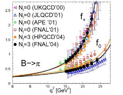
Figure 4: Form factors for $B\rightarrow\pi\ell\nu$ computed by simulations of lattice QCD[16].

The determination of $|V_{ub}|$ from exclusive decays requires a priori knowledge of the form factors for $B\rightarrow\pi$ and/or $B\rightarrow\rho$, e.g.,

$$\langle\pi(p_{\pi})|\overline{b}\gamma_{\mu}q|B(P_{B})\rangle=\left((p_{B}+p_{\pi})_{\mu}-\frac{m_{B}^{2}-m_{\pi}^{2}}{q^{2}}q_{\mu}\right){F_{+}(q^{2})}+\frac{m_{B}^{2}-m_{\pi}^{2}}{q^{2}}q_{\mu}{F_{0}(q^{2})}\,.$$ (9)

HQET does not fix normalization at zero recoil as it does in $B\rightarrow D^{(*)}\ell\nu$. Analyticity and unitarity do constrain the functional form, which helps, e.g., to interpolate lattice results. An interpolation of lattice results is shown in Fig. 4. One can use this to determine $|V_{ub}|$, but the errors are large. Belle finds, from $B\rightarrow\pi\ell\nu$ restricted to $q^{2}>16\text{GeV}^{2}$, $|V_{ub}|=(3.87\pm 0.70\pm 0.22^{+0.85}_{-0.51})\times 10^{-3}$ and $|V_{ub}|=(4.73\pm 0.85\pm 0.27^{+0.74}_{-0.50})\times 10^{-3}$ using lattice results from FNAL’04 and HPQCD, respectively[23]. The theory errors, $\sim\pm 20$%, are not expected to be significantly reduced soon. There has also been some effort to understand the precision with which $|V_{td}|$ can be determined from $B\rightarrow\rho\gamma$ decays[24].

New ideas are needed to reduce the error on $|V_{ub}|$ from exclusive decays to the sub-10% level, hopefuly to a few percent. One recent proposal[25] is to use double ratios[26] to eliminate hadronic uncertainties. A double-ratio is a ratio of ratios of quantities that are fixed by two symmetries. For example,

$$R_{1}={\frac{f_{B_{s}}/f_{B}}{f_{D_{s}}/f_{D}}}={\frac{f_{B_{s}}/f_{D_{s}}}{f_{B}/f_{D}}}=1+{\cal O}\left(m_{s}\left(\frac{1}{m_{c}}-\frac{1}{m_{b}}\right)\right)$$ (10)

The ratios $f_{B_{s}}/f_{B}$ and $f_{D_{s}}/f_{D}$ are unity in the flavor-$SU(3)$ limit, while the ratios $f_{B_{s}}/f_{D_{s}}$ and $f_{B}/f_{D}$ are fixed to $\sqrt{m_{c}/m_{b}}$ by heavy-quark symmetry. Hence $R_{1}-1$ vanishes either as $m_{s}\rightarrow 0$ or as $m_{Q}\rightarrow\infty$, as indicated.

To use a double-ratio in a precise determination of $|V_{ub}/V_{tb}V_{ts}|$, one measures, for $4m_{c}^{2}<q^{2}\lesssim q^{2}_{\rm max}=(m_{B}-m_{\rho,K^{*}})^{2}$

$$\frac{\mbox{d}\Gamma(\overline{B}\rightarrow\rho e\nu)/\mbox{d}q^{2}}{\mbox{d}\Gamma(\overline{B}\rightarrow K^{*}\ell^{+}\ell^{-})/\mbox{d}q^{2}}={\frac{|V_{ub}|^{2}}{|V_{tb}V_{ts}^{*}|^{2}}}\cdot\frac{8\pi^{2}}{\alpha^{2}}\cdot\frac{1}{N_{\rm eff}(q^{2})}\frac{\sum_{\lambda}|H_{\lambda}^{B\rightarrow\rho}(q^{2})|^{2}}{\sum_{\lambda}|H_{\lambda}^{B\rightarrow K^{*}}(q^{2})|^{2}}\,.$$ (11)

Here $H_{\lambda}$ are helicity amplitudes, and $N_{\rm eff}(q^{2})$ is a calculable function that incorporates the effects of penguin diagrams. In addition one must measure decay spectra for $D\rightarrow\rho\ell\nu$ and $D\rightarrow K^{*}\ell\nu$ and express all rates as functions of $y=E_{V}/m_{V}$ ($V=\rho,K^{*}$). Then one uses double-ratio magic. Let

$$R_{B\rightarrow V}(y)\equiv\frac{\sum_{\lambda}|H_{\lambda}^{B\rightarrow\rho}(y)|^{2}}{\sum_{\lambda}|H_{\lambda}^{B\rightarrow K^{*}}(y)|^{2}}\qquad\qquad R_{D\rightarrow V}(y)\equiv\frac{\sum_{\lambda}|H_{\lambda}^{D\rightarrow\rho}(y)|^{2}}{\sum_{\lambda}|H_{\lambda}^{D\rightarrow K^{*}}(y)|^{2}}$$ (12)

then

$$R_{B\rightarrow V}(y)=R_{D\rightarrow V}(y)\Big{(}1+{\cal O}(m_{s}(\frac{1}{m_{c}}-\frac{1}{m_{b}}))\Big{)}$$ (13)

can be used to eliminate the unknown helicity amplitudes from the analysis.

For the calculation of the factor $N_{\rm eff}(q^{2})=|C_{9}^{\rm eff}+\frac{2m_{b}^{2}}{q^{2}}C_{7}^{\rm eff}|^{2}+|C_{10}|^{2}+O(\mathchar 28931\relax/m_{b})$, one may include the effects of penguin diagrams through an OPE. This is indicated above through the superscript “eff” ($C_{7,9}\rightarrow C_{7,9}^{\rm eff}$). In applying the OPE, there is no need to assume that the four quark operators factorize into the product of two currents. However, the OPE is used in the timelike region, so this assumes local duality. The situation is under fairly good control, however, since the penguin contribution is very small compared to the leading contribution from the contact terms. Although the contribution is small, it is crucial to include it in order to minimize the scale dependence of $N_{\rm eff}(q^{2})$. The uncertainty in the scale dependence in $N_{\rm eff}(q^{2})$, which should be an RG-invariant, is only a couple of percent in a NNLO calculation.

Although a comprehensive study of the corrections has not been performed, preliminary estimates indicate that the theoretcial error in the determination of $|V_{ub}|$ could well be bellow 10% with this method. For example, the deviation of $R_{1}$ from 1 is about 2% in model and lattice calculations[27]. Similar results are obtained for the double ratio of form factors for $B/D\rightarrow K^{*}/\rho$[28].

References

• [1] Sasha Glazov, these proceedings pp. LABEL:GlazovStartLABEL:GlazovEnd
• [2] Pyungwon Ko, these proceedings, pp.LABEL:KoStartLABEL:KoEnd
• [3] Alex Lenz, these proceedings pp. LABEL:LenzStartLABEL:LenzEnd
• [4] S. Eidelman et al. [Particle Data Group Collaboration], Phys. Lett. B 592, 1 (2004).
• [5] J. Chay, H. Georgi and B. Grinstein, Phys. Lett. B 247, 399 (1990).
• [6] M. Battaglia et al., Phys. Lett. B 556, 41 (2003)
• [7] P. Gambino and N. Uraltsev, Eur. Phys. J. C 34, 181 (2004)
• [8] C. W. Bauer, Z. Ligeti, M. Luke, A. V. Manohar and M. Trott, arXiv:hep-ph/0408002.
• [9] A. X. El-Khadra and M. Luke, Ann. Rev. Nucl. Part. Sci.  52, 201 (2002)
• [10] Elisabetta Barberio, these proceedings pp. LABEL:BarberioStartLABEL:BarberioEnd
• [11] A. H. Hoang, arXiv:hep-ph/0008102.
• [12] C. G. Boyd, B. Grinstein and R. F. Lebed, Phys. Rev. D 56, 6895 (1997); idem, Nuovo Cim.  109A, 863 (1996); idem, Nucl. Phys. B 461, 493 (1996); idem, Phys. Lett. B 353, 306 (1995)
• [13] I. Caprini and M. Neubert, Phys. Lett. B 380, 376 (1996); I. Caprini, L. Lellouch and M. Neubert, Nucl. Phys. B 530, 153 (1998)
• [14] N. Uraltsev, Phys. Lett. B 501, 86 (2001); A. Le Yaouanc, L. Oliver and J. C. Raynal, Phys. Lett. B 557, 207 (2003); M. P. Dorsten, arXiv:hep-ph/0310025.
• [15] P. F. Harrison and H. R. Quinn, “The BaBar physics book: Physics at an asymmetric B factory,” SLAC-R-0504
• [16] M. Okamoto, these proceedings pp. LABEL:OkamotoStartLABEL:OkamotoEnd
• [17] B. Grinstein and Z. Ligeti, Phys. Lett. B 526, 345 (2002);
• [18] M. P. Dorsten, Phys. Rev. D 70, 096013 (2004)
• [19] A. K. Leibovich, I. Low and I. Z. Rothstein, Phys. Rev. D 61, 053006 (2000); Phys. Lett. B 486, 86 (2000);
• [20] C. W. Bauer, Z. Ligeti and M. E. Luke, arXiv:hep-ph/0101328.
• [21] K. S. M. Lee and I. W. Stewart, arXiv:hep-ph/0409045.
• [22] C. W. Bauer, M. Luke and T. Mannel, Phys. Lett. B 543, 261 (2002); C. W. Bauer, Z. Ligeti and M. E. Luke,Phys. Rev. D 64, 113004 (2001); A. K. Leibovich, Z. Ligeti and M. B. Wise, Phys. Lett. B 539, 242 (2002)
• [23] K. Abe et al. [BELLE Collaboration], arXiv:hep-ex/0408145.
• [24] B. Grinstein and D. Pirjol, Phys. Rev. D 62 (2000) 093002; M. Beneke, T. Feldmann and D. Seidel, Nucl. Phys. B 612 (2001) 25; S. W. Bosch and G. Buchalla, Nucl. Phys. B 621 (2002) 459; A. Ali and A. Y. Parkhomenko, Eur. Phys. J. C 23 (2002) 89
• [25] B. Grinstein and D. Pirjol, arXiv:hep-ph/0404250; Z. Ligeti and M. B. Wise, Phys. Rev. D 53, 4937 (1996)
• [26] B. Grinstein, Phys. Rev. Lett.  71, 3067 (1993)
• [27] G. Cvetic, C. S. Kim, G. L. Wang and W. Namgung, Phys. Lett. B 596, 84 (2004)
• [28] Z. Ligeti, I. W. Stewart and M. B. Wise, Phys. Lett. B 420, 359 (1998) [arXiv:hep-ph/9711248].