Leptonic CP violation in a two parameter model

Abstract

We further study the “complementary” Ansatz, Tr$(M_{\nu})$=0, for a prediagonal light Majorana type neutrino mass matrix. Previously, this was studied for the CP conserving case and the case where the two Majorana type CP violating phases were present but the Dirac type CP violating phase was neglected. Here we employ a simple geometric algorithm which enables us to “solve” the Ansatz including all three CP violating phases. Specifically, given the known neutrino oscillation data and an assumed two parameter (the third neutrino mass $m_{3}$ and the Dirac CP phase $\delta$) family of inputs we predict the neutrino masses and Majorana CP phases. Despite the two parameter ambiguity, interesting statements emerge. There is a characteristic pattern of interconnected masses and CP phases. For large $m_{3}$ the three neutrinos are approximately degenerate. The only possibility for a mass hierarchy is to have $m_{3}$ smaller than the other two. A hierarchy with $m_{3}$ largest is not allowed. Small CP violation is possible only near two special values of $m_{3}$. Also, the neutrinoless double beta decay parameter is approximately bounded as 0.020 eV $<|m_{ee}|<$ 0.185 eV. As a byproduct of looking at physical amplitudes we discuss an alternative parameterization of the lepton mixing matrix which results in simpler formulas. The physical meaning of this parameterization is explained.

I Introduction

The remarkable experimental achievements (for some recent examples see refs. kamland ; sno ; k2k ) relating to neutrino oscillations nos have brought much closer to reality the goal of determining the “light” neutrino masses and the presumed 3 $\times$ 3 lepton mixing matrix. It is possible that more than three light neutrinos are required in order to understand the results of the LSND experiment lsnd . However, we consider it reasonable, before deciding on this, to wait for further supporting evidence as should be supplied soon by the MiniBooNE collaboration mbc . The mixing matrix contains three mixing angles and, if the neutrinos are considered to be Dirac type fermions, a single CP violation phase. That would be completely analogous to the situation prevailing in the quark sector of the electroweak theory. But it seems very interesting to consider the possibility that the three light neutrinos are Majorana type fermions. This involves only half as many fermionic degrees of freedom and would be mandated if neutrinoless double beta decay were to be conclusively established. The Majorana neutrino scenario implies the existence of two additional CP violation phasessv ; bhp ; dknot ; svandgkm . Then nine quantities (beyond the charged lepton masses) would be required for the specification of the lepton sector: three neutrino masses, three mixing angles and three CP violation phases.

According to a recent analysis mstv it is possible to extract from the data to good accuracy, two squared neutrino mass differences: $m_{2}^{2}-m_{1}^{2}$ and $|m_{3}^{2}-m_{2}^{2}|$, and two inter-generational mixing angle squared sines: $s_{12}^{2}$ and $s_{23}^{2}$. Furthermore the inter-generational mixing parameter $s_{13}^{2}$ is found to be very small. Thus 5 out of 9 quantities needed to describe the leptonic sector in the Majorana neutrino scenario can be considered as “known”. For many purposes it is desirable to get an idea of the remaining 4 parameters. As an aid in partially determining the other parameters, a so-called “complementary Ansatz” was proposed bfns ; hz ; ro ; nsm . The name arises from the fact that if CP violation is neglected, the Ansatz determines (up to two different cases) all three neutrino masses, given the two known squared mass differences.

This complementary Ansatz simply reads,

$$Tr(M_{\nu})=0.$$ (1)

Here $M_{\nu}$ is the symmetric, but in general complex, prediagonal Majorana neutrino mass matrix. It is brought to diagonal form by the transformation,

$$U^{T}M_{\nu}U=diag(m_{1},m_{2},m_{3})={\hat{M}_{\nu}},$$ (2)

where $U$ is a unitary matrix and the $m_{i}$ may be chosen as real, positive. We impose the condition in a basis where the charged leptons are diagonal so that U gets identified with the lepton mixing matrix.

Since Eq. (1) comprises two real equations, it gives two conditions on the unknown 4 parameters of the lepton sector. In other words, the lepton sector is described by a two parameter family of solutions. This can be approximately simplified bfns ; ro ; nsm by noting that the effects of one CP violation phase get suppressed when the small quantity $s_{13}$ vanishes. Then there is a one parameter family of solutions describing the lepton sector and it is straightforward to compute physical quantities for parameter choices which span this family. The main purpose of the present paper is to find the general solutions of Eq. (1) without making this approximation. This gives a two parameter family which allows one to study the interplay of all three CP violation phases.

A plausibility argument supporting the complementary Ansatz is concisely presented in sections 2 and 3 of nsm2 . It is based on using the SO(10) grand unification group in the approximation that the non-seesaw neutrino mass term dominates. The Higgs fields which can contribute to fermion masses at tree level are the 10, 120 and the 126. If only a single 126 appears (but any number of the others) one has the relation

$$Tr(M^{D}-rM^{E})\propto Tr(M_{\nu}),$$ (3)

where $M^{D}$ and $M^{E}$ are, respectively, the prediagonal mass matrices of the charge -1/3 quarks and charge -1 leptons, while $r\approx$ 3 takes account of running masses from the grand unified scale to about 1 GeV. Now one of the major surprises generated by the neutrino oscillation experiments is that, unlike the quark mixing matrix which has the form diag (1,1,1) + O$(\epsilon)$, the lepton mixing matrix is not at all close to the unit matrix. This suggests a further approximation in which one takes $M^{D}$ and $M^{E}$ to be diagonal but allows the neutrino mass matrix to be far from the unit matrix. Then the left hand side of Eq. (3) is approximately $(m_{b}-3m_{\tau})$, which is in turn close to zero.

As we will see, the model makes a number of characteristic predictions for the neutrino mass spectrum which should enable it to be readily tested in the near future. A very recent review of many other models is given in ref. metal .

For convenience, our notation (essentially the standard one) for the lepton mixing matrix and the corresponding parameterized Ansatz is given in section II.

In section III the Ansatz is solved in the sense of providing a geometrical algorithm which, given the two input quantities $m_{3}$ (third neutrino mass, taken positive) and $\delta$ (conventional CP violation phase in the lepton mixing matrix), enables one to predict the other two neutrino masses as well as the other two CP violation phases. Of course, the experimental knowledge on the neutrino squared mass differences and CP conserving intergenerational mixing angles are taken to be “known”. We separate the solutions into two types I and II, depending respectively on whether $m_{3}$ is the largest or the smallest of the neutrino masses. In addition, there is a discrete ambiguity corresponding to reflecting a triangle involved in the algorithm. A “panoramic” view of the predictions as functions of $m_{3}$ and $\delta$ are presented in a convenient tabular form. The greatest allowed value of $m_{3}$ is determined by a cosmology bound. As $m_{3}$ decreases, a point is reached at which the type I solutions no longer exist. As $m_{3}$ decreases even further, the type II solutions also cease to exist. The corresponding values of $m_{3}$ at which these solutions become disallowed depend on the assumed value of the input $\delta$. This correlation is studied analytically.

Some physical considerations are discussed in section IV. First, the dependence on the experimentally bounded squared mixing angle, $s_{13}^{2}$ is investigated. We present also a chart showing the dependence of the neutrinoless double beta decay parameter $|m_{ee}|$ on the input parameters $m_{3}$ and $\delta$. Even though the inputs are varying over a fairly large range, the rather restrictive approximate bounded range 0.020 eV $<|m_{ee}|<$ 0.185 eV emerges from the Ansatz.

After calculating observable quantities in the model one observes that they depend more simply on certain linear combinations of the conventional “Dirac” and “Majorana” CP violation phases. In section V we discuss an alternative parameterization of the lepton mixing matrix in which these combinations occur directly. In this parameterization the three phases just correspond to the three possible intergenerational mixings. An “invariant” combination of these three corresponds to the usual “Dirac” phase $\delta$.

We conclude in section VI which contains a brief summary and a discussion of results which emphasize some unique features of the present work.

II Parameterized complementary Ansatz

We define the lepton mixing matrix, $K$ from the charged gauge boson interaction term in the leptonic sector of the electroweak Lagrangian:

$${\cal L}=\frac{ig}{\sqrt{2}}W_{\mu}^{-}{\bar{e}_{L}}\gamma_{\mu}K\nu+H.c..$$ (4)

Note that the “mass diagonal” neutrino fields, $\nu_{i}$ are related to the fields, $\rho_{i}$ in the prediagonal mass basis by the matrix equation,

$$\rho=U\nu.$$ (5)

We adopt essentially what seems to be the most common parameterization:

$$K=K_{exp}\omega_{0}^{-1}(\tau),$$ (6)

where a unimodular diagonal matrix of phases is defined as,

$$\omega_{0}(\tau) = diag(e^{i\tau_{1}},e^{i\tau_{2}},e^{i\tau_{3}}),$$

$$\tau_{1}+ \tau_{2} +\tau_{3}=0.$$ (7)

The remaining factor, $K_{exp}$ which is the only part needed for describing ordinary neutrino oscillations is written as the product of three successive two dimensional unitary transformations,

$$K_{exp}=\omega_{23}(\theta_{23},0)\omega_{13}(\theta_{13},-\delta)\omega_{12}(\theta_{12},0),$$ (8)

with three mixing angles and the CP violation phase $\delta$. For example in the (12) subspace one has:

$$\omega_{12}(\theta_{12},\phi_{12})=\left[\begin{array}[]{c c c}cos\theta_{12}&e^{i\phi_{12}}sin\theta_{12}&0\\ -e^{-i\phi_{12}}sin\theta_{12}&cos\theta_{12}&0\\ 0&0&1\end{array}\right]$$ (9)

with clear generalization to the (23) and (13) transformations. Multiplying out yields:

$$K_{exp}=\left[\begin{array}[]{c c c}c_{12}c_{13}&s_{12}c_{13}&s_{13}e^{-i\delta}\\ -s_{12}c_{23}-c_{12}s_{13}s_{23}e^{i\delta}&c_{12}c_{23}-s_{12}s_{13}s_{23}e^{i\delta}&c_{13}s_{23}\\ s_{12}s_{23}-c_{12}s_{13}c_{23}e^{i\delta}&-c_{12}s_{23}-s_{12}s_{13}c_{23}e^{i\delta}&c_{13}c_{23}\\ \end{array}\right]$$ (10)

where $s_{ij}=sin\theta_{ij}\;and\;c_{ij}=cos\theta_{ij}$.

Identifying $K$ with $U$ in Eq. (2), the Ansatz of Eq. (1) now reads,

$$Tr({\hat{M}_{\nu}}K_{exp}^{-1}K_{exp}^{*}\omega_{0}(2\tau))=0,$$ (11)

where Eqs. (2) and (6) were used. With the parameterized mixing matrix of Eq. (10) the Ansatz finally becomes:

$$m_{1}e^{2i\tau_{1}}\left[1-2i(c_{12}s_{13})^{2}sin{\delta}e^{-i\delta}\right]+$$

$$m_{2}e^{2i\tau_{2}}\left[1-2i(s_{12}s_{13})^{2}sin{\delta}e^{-i\delta}\right]+$$

$$m_{3}e^{2i\tau_{3}}\left[1+2i(s_{13})^{2}sin{\delta}e^{i\delta}\right]=0.$$ (12)

In this equation we can choose the diagonal masses $m_{1},m_{2},m_{3}$ to be real positive. Notice that setting the mixing parameter $s_{13}$ to zero eliminates the dependence on the CP violation phase $\delta$. Then Eq. (12) goes over to the simpler form studied previously nsm .

III Solving the Ansatz in the general case

For definiteness we will use the following best fit values for the differences of squared neutrino masses obtained in ref. mstv :

$$A\equiv m_{2}^{2}-m_{1}^{2} = 6.9\times 10^{-5}eV^{2},$$

$$B\equiv|m_{3}^{2}-m_{2}^{2}| = 2.6\times 10^{-3}eV^{2}.$$ (13)

The uncertainty in these determinations is roughly $25\%$. Similarly for definiteness we will adopt the best fit values for $s_{12}^{2}$ and $s_{23}^{2}$ obtained in the same analysis:

$$s_{12}^{2}=0.30,\quad s_{23}^{2}=0.50.$$ (14)

These mixing angles also have about a $25\%$ uncertainty. The experimental status of $s_{13}^{2}$ is less accurately known. At present only the 3 $\sigma$ bound,

$$s_{13}^{2}\leq 0.047,$$ (15)

is available. For our discussion we will consider $s_{13}^{2}$ to be known at a “typical” value satisfying this bound and examine the sensitivity to changing it. Of course, the experimental determination of $s_{13}$ is a topic of great current interest.

Previouslynsm , the (positive) mass of the third neutrino, $m_{3}$ was considered to be the free parameter. It was varied to obtain, via the simplified Ansatz equation, a “panoramic view” of the two independent Majorana phases (say $\tau_{1}$ and $\tau_{2}$). In the present case, we shall not neglect the CP violation phase $\delta$ and consider it too as a free parameter to be varied. It is necessary to specify a suitable algorithm to treat the full Ansatz. Previously it was noted that the simplified Ansatz could be pictured as a vector triangle in the complex plane having sides equal to corresponding neutrino masses (See Fig. 1 of nsm ). The three internal angles were found by trigonometry and related to the three angles made by the sides with respect to the positive real axis. Those in turn were twice the three (constrained) Majorana phases. The orientation of the triangle got determined (up to a reflection) by the constraint in Eq. (7). In the present case we will also rewrite the Ansatz equation as a vector triangle in the complex plane. However the sides will differ from the neutrino masses. In addition the angles will differ from twice the constrained Majorana phases.

To start, we choose a value for $m_{3}$ and a value for the phase $\delta$. Then we can obtain from Eqs.(13) two different solutions for the other masses $m_{1}$ and $m_{2}$. We call the solution where $m_{3}$ is the largest neutrino mass, the type I case. The case where $m_{3}$ is the smallest neutrino mass is designated type II. $m_{1}$ will be determined from the assumed value of $m_{3}$ as,

$$m_{1}^{2}=m_{3}^{2}-A\mp B,$$ (16)

where the upper and lower sign choices respectively refer to the type I and type II cases. In either case we find $m_{2}$ as,

$$m_{2}^{2}=A+m_{1}^{2}.$$ (17)

.

Next, we redefine variables so that each of the three terms in the Ansatz equation, (12) is characterized by a single magnitude, $m_{i}^{\prime}$ and a single phase, $2\tau_{i}^{\prime}$. Eq. (12) then reads,

$$m_{1}^{\prime}e^{2i\tau_{1}^{\prime}}+m_{2}^{\prime}e^{2i\tau_{2}^{\prime}}+m_{3}^{\prime}e^{2i\tau_{3}^{\prime}}=0.$$ (18)

This equation evidently represents a vector triangle in the complex plane, as illustrated in Fig. 1.

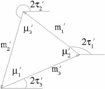
Figure 1: Vector triangle representing Eq. (18).

However the lengths are not the physical neutrino masses and the phases are not twice the physical Majorana CP violation phases. The auxiliary, primed, masses are seen to be related to the (now known) physical masses by,

$$m_{i}^{\prime}=G_{i}m_{i},$$ (19)

where,

$$G_{1} = \left[1-4\left(c_{12}s_{13}\right)^{2}\sin^{2}\delta+4\left(c_{12}s_{13}\right)^{4}\sin^{2}\delta\right]^{1/2},$$

$$G_{2} = \left[1-4\left(s_{12}s_{13}\right)^{2}\sin^{2}\delta+4\left(s_{12}s_{13}\right)^{4}\sin^{2}\delta\right]^{1/2},$$

$$G_{3} = \left[1-4s_{13}^{2}\sin^{2}\delta+4s_{13}^{4}\sin^{2}\delta\right]^{1/2}.$$ (20)

Notice that, since $\delta$ has already been specified, the relations between the $m_{i}^{\prime}$ and the $m_{i}$ are now known. Similarly, the physical phases are related to the primed ones by,

$$\tau_{i}=\tau_{i}^{\prime}+F_{i},$$ (21)

where,

$$F_{1} = \frac{1}{2}\arctan\frac{\left(c_{12}s_{13}\right)^{2}\sin(2\delta)}{1-2\left(c_{12}s_{13}\right)^{2}\sin^{2}\delta},$$

$$F_{2} = \frac{1}{2}\arctan\frac{\left(s_{12}s_{13}\right)^{2}\sin(2\delta)}{1-2\left(s_{12}s_{13}\right)^{2}\sin^{2}\delta},$$

$$F_{3} = -\frac{1}{2}\arctan\frac{s_{13}^{2}\sin(2\delta)}{1+2s_{13}^{2}\sin^{2}\delta}.$$ (22)

Again, note that, since $\delta$ has been specified, the relations between the $\tau_{i}$ and the $\tau_{i}^{\prime}$ are now known. Referring to Fig. 1 we can determine the internal angles, $\mu_{i}^{\prime}$ by using the law of cosines. For example,

$$cos\mu_{1}^{\prime}=\frac{-(m_{1}^{\prime})^{2}+(m_{2}^{\prime})^{2}+(m_{3}^{\prime})^{2}}{2m_{2}^{\prime}m_{3}^{\prime}}.$$ (23)

Next, the auxiliary phases $\tau_{i}^{\prime}$ can be related to the internal angles just obtained as:

$$\tau_{1}^{\prime} = \frac{1}{6}(\pi-\mu_{1}^{\prime}-2\mu_{2}^{\prime})+\rho,$$

$$\tau_{2}^{\prime} = \frac{1}{6}(\pi+2\mu_{1}^{\prime}+\mu_{2}^{\prime})+\rho,$$

$$\tau_{3}^{\prime} = \frac{1}{6}(-2\pi-\mu_{1}^{\prime}+\mu_{2}^{\prime})+\rho.$$ (24)

The remaining still unknown parameter here is $\rho$ which we added to the right hand side of each equation. It represents the effect of an arbitrary rotation of the whole triangle, which should not be determinable from the internal angles. It can be determined, however, by making use of the constraint on the physical phases, $\sum_{i}\tau_{i}=0$. Notice that there is no corresponding constraint for $\sum_{i}\tau_{i}^{\prime}$. Using Eq. (21) we get,

$$\rho=-\frac{1}{3}\sum_{i}F_{i},$$ (25)

where the $F_{i}$ are to be read from Eqs. (22). Now the masses $m_{1},m_{2}$ and the phases $\tau_{1},\tau_{2}$ have been determined by a simple algorithm, upon specification of $m_{3}$ and $\delta$.

As remarked above, the dependence on the CP violation phase $\delta$ is suppressed in the limit that the mixing parameter $s_{13}^{2}$ vanishes. Hence, to illustrate this new feature, we will consider a value $s_{13}^{2}$ =0.04, close to the 3$\sigma$ upper bound of 0.047 mstv . The predictions of the neutrino masses $(m_{1},m_{2})$ and two independent phases $(\tau_{1},\tau_{2})$, from the Ansatz for various assumed values of $m_{3}$ and $\delta$ are given in Table 1. Representative values of $\delta$ were chosen to lie between 0 and $\pi$ since it may be observed from Eqs. (20) and (22) that the solutions will have a periodicity of $\pi$ with respect to $\delta$. Just from the Ansatz there is no upper bound on the value of $m_{3}$. However there is a recent cosmological bound cosmobound which requires,

$$|m_{1}|+|m_{2}|+|m_{3}|<0.7\textrm{ eV}.$$ (26)

Thus values of $m_{3}$ greater than about 0.3 eV are physically disfavored. Table 1 shows that at this value both type I and type II solutions exist. This is true also for higher values of $m_{3}$. The picture remains very similar down to around $m_{3}=0.1$ eV but as one gets closer to roughly $0.06$ eV, there is a marked change. If one further lowers $m_{3}$, it is found that the type I solution no longer exists. On the other hand the type II solution persists and does not change much until $m_{3}$ approaches the neighborhood of 0.001 eV. There are no solutions for $m_{3}$ below this region.

type	$m_{1},m_{2},m_{3}$ in eV	$\tau_{1},\tau_{2}(\delta=0)$	$\tau_{1},\tau_{2}(\delta=0.5)$	$\tau_{1},\tau_{2}(\delta=1.0)$	$\tau_{1},\tau_{2}(\delta=1.5)$	$\tau_{1},\tau_{2}(\delta=2.0)$	$\tau_{1},\tau_{2}(\delta=2.5)$
I	0.2955, 0.2956, 0.3	0.0043,1.0428	0.0126, 1.0495	0.0058, 1.0536	-0.0108, 1.0510	-0.0210, 1.0440	-0.0153, 1.0394
II	0.3042, 0.3043, 0.3	-0.0041,1.0512	0.0043,1.0577	-0.0023, 1.0615	-0.0189, 1.0587	-0.0291,1.0518	-0.0235,1.0476
I	0.0856, 0.0860, 0.1	0.0486, 0.9975	0.0566, 1.0049	0.0489, 1.0106	0.0318, 1.0091	0.0219,1.0015	0.0285,0.9953
II	0.1119, 0.1123, 0.1	-0.0311, 1.0774	-0.0226, 1.0835	-0.0289, 1.0863	-0.0453, 1.0828	-0.0556,1.0763	-0.0503,1.0731
I	0.0305, 0.0316, 0.06	0.3913, 0.6543	0.3873, 0.6748	0.3578, 0.7048	0.3288, 0.7167	0.3258,0.7013	0.3530,0.6720
II	0.0783, 0.0787, 0.06	-0.0669, 1.1119	-0.0583, 1.1174	-0.0644,1.1188	-0.0806, 1.1145	-0.0911,1.1085	-0.0860,1.1066
II	0.0643, 0.0648, 0.04	-0.1064, 1.1494	-0.0978, 1.1541	-0.1040, 1.1538	-0.1203, 1.1483	-0.1307,1.1430	-0.1255,1.1428
II	0.0541, 0.0548, 0.02	-0.1747, 1.2115	-0.1669, 1.2142	-0.1751, 1.2095	-0.1928, 1.2012	-0.2024,1.1976	-0.1951,1.2019
II	0.0506, 0.0512, 0.005	-0.2601, 1.2620	-0.2603, 1.2611	-0.2914, 1.2276	-0.3251, 1.2035	-0.3250,1.2094	-0.2950,1.2369
II	0.0503, 0.0510, 0.001	-0.3830, 1.1805

Table 1: Panorama of solutions as $m_{3}$ is lowered from about the highest value which is experimentally reasonable to about the lowest value imposed by the model. For each value of $m_{3}$, predictions are given for $(m_{1},m_{2})$ and for $(\tau_{1},\tau_{2})$ in the cases where $\delta=0,0.5,1.0,1.5,2.0,2.5$. All phases are measured in radians. Here the value $s_{13}^{2}$ =0.04 was adopted. In the type I solutions $m_{3}$ is the largest mass while in the type II solutions $m_{3}$ is the smallest mass.

Note that the columns in Table 1 with $\delta=0$ correspond to the previous case, discussed in some detail in section IV of nsm . In this case, $m_{i}^{\prime}$ and $\tau_{i}^{\prime}$ respectively coincide with $m_{i}$ and $\tau_{i}$ so we can identify the vectors of the triangle with the physical masses and phases. As one decreases the value of $m_{3}$ the type I triangle goes from being close to equilateral to the degenerate situation with three collinear vectors. In this limiting case the vectors representing neutrino one and neutrino two are approximately equal and add up to exactly cancel the vector representing neutrino 3. The precise orientation of the straight line is due to imposing the constraint in Eq. (7). This is actually a CP conserving case realcase . Then one can find the $m_{3}$ value (a little below 0.06 eV) for this situation by looking for a real solution of $m_{1}+m_{2}+m_{3}=0$ together with Eqs. (13) (See Eq. (4.4) of bfns ). Clearly there can be no type I solutions below this value of $m_{3}$. The type II solutions can exist below this value but similarly end (a little below $m_{3}$ =0.001 eV) when the triangle becomes degenerate in a different way. For the type II degenerate triangle, the neutrino 1 and neutrino 2 vectors are collinear but oppositely directed and the small neutrino 3 vector adds to the neutrino 1 vector to cancel the neutrino 2 vector. This is also a CP conserving case.

When the effects of $\delta$ not equal to zero are included, it is not possible to make a triangle out of the physical neutrino masses and phases. The relevant auxiliary triangle is made, as illustrated, using the primed masses and phases. Thus the limiting values of $m_{3}$, where the type I and type II cases each end, correspond to this primed triangle becoming degenerate. We can get the limiting value by looking for real solutions of $\sum_{i}G_{i}m_{i}$=0, together with Eqs. (13). The limiting value, $(m_{3})_{min}$ is found to be:

$$(m_{3})_{min}^{2}=\frac{1}{2\alpha}[-\beta-(\beta^{2}-4\alpha\gamma)^{1/2}],$$ (27)

where,

$$\alpha = (G_{1}^{2}+G_{2}^{2}-G_{3}^{2})^{2}-4G_{1}^{2}G_{2}^{2},$$

$$\beta = -2(G_{1}^{2}+G_{2}^{2}-G_{3}^{2})(AG_{1}^{2}\pm B(G_{1}^{2}+G_{2}^{2}))+4G_{1}^{2}G_{2}^{2}(A\pm 2B),$$

$$\gamma = (AG_{1}^{2}\pm B(G_{1}^{2}+G_{2}^{2}))^{2}\mp 4G_{1}^{2}G_{2}^{2}B(A\pm B).$$ (28)

Here the upper and lower sign choices respectively refer to the type I and type II cases.

The computed values of $(m_{3})_{min}$ as a function of $\delta$ are shown in Table 2. Looking at this table, one can see why the entries in Table 1 for $m_{3}$ =0.001 eV and non-zero values of $\delta$ are missing. Simply, for those cases, $(m_{3})_{min}>$ 0.001 eV. Clearly, this correlation of the allowed input values of $m_{3}$ with the input values of $\delta$ must be respected in studying the present model. This correlation is imposed by the Ansatz itself. For large values of $m_{3}$ there is no constraint from the Ansatz but Eq. (26) gives an experimental constraint. It should be remarked that the collinear auxiliary triangles with non-zero $\delta$ correspond to CP violation. In these cases the CP violation arises from non trivial phases, $\tau_{i}$ in addition to the assumed non-zero $\delta$. Actually, a better measure of CP violation involves the (two independent) phase differences $\tau_{i}-\tau_{j}$. These are the objects essentially related to the internal angles in Fig. 1.

type	$(m_{3})_{min}$ $(\delta=0)$ in eV	$(m_{3})_{min}$ $(\delta=0.5)$	$(m_{3})_{min}$ $(\delta=1.0)$	$(m_{3})_{min}$ $(\delta=1.5)$	$(m_{3})_{min}$ $(\delta=2.0)$	$(m_{3})_{min}$ $(\delta=2.5)$
I	0.0592716	0.0590967	0.0587178	0.0584799	0.0586203	0.0589971
II	0.0006811	0.00105461	0.0019024	0.0024636	0.0021294	0.0012723

Table 2: Minimum allowed value of the input mass, $m_{3}$ as a function of the input CP violation phase, $\delta$. These correspond to the cases where the triangle in Fig. 1 becomes degenerate. Here, the choice $s_{13}^{2}=$ 0.04 has been made.

As noted in ref nsm , the possibility of reflecting the triangle about any line in the plane gives another set of solutions corresponding to reversing the signs of all the phase differences $\tau_{i}-\tau_{j}$. In the present case, where $\delta$ is not zero, reflecting the “unphysical” triangle about any line in the plane will give an alternate solution in which the $\tau_{i}^{\prime}-\tau_{j}^{\prime}$ are reversed in sign. More specifically, one should reverse the signs of the first terms on the right hand sides in Eqs. (24). The physical phases, $\tau_{i}$ for this alternate solution will then depend on $\delta$ as illustrated in Table 3.

type	$m_{3}$ in eV	$\tau_{1},\tau_{2}(\delta=0)$	$\tau_{1},\tau_{2}(\delta=0.5)$	$\tau_{1},\tau_{2}(\delta=1.0)$	$\tau_{1},\tau_{2}(\delta=1.5)$	$\tau_{1},\tau_{2}(\delta=2.0)$	$\tau_{1},\tau_{2}(\delta=2.5)$
I	0.3	-0.0043,-1.0428	0.0113,-1.0393	0.0210, -1.0422	0.0151, -1.0492	-0.0015, -1.0536	-0.0123, -1.0512
II	0.3	0.0041,-1.0512	0.0196, -1.0475	0.0291, -1.0500	0.0232, -1.0569	0.0066, -1.0614	-0.0040, -1.0593
I	0.1	-0.0486, -0.9975	-0.0326, -0.9947	-0.0221, -0.9992	-0.0275, -1.0073	-0.0444, -1.0111	-0.0560, -1.0070
II	0.1	0.0311, -1.0774	0.0465, -1.0732	0.0557, -1.0748	0.0495, -1.0810	0.0331, -1.0859	0.0228, -1.0848
I	0.06	-0.3913, -0.6543	-0.3634, -0.6645	-0.3310, -0.6934	-0.3246, -0.7149	-0.3483, -0.7109	-0.3806,-0.6837
II	0.06	0.0669, -1.1119	0.0822, -1.1071	0.0912, -1.1073	0.0849, -1.1127	0.0685, -1.1180	0.0584, -1.1183
II	0.04	0.1064, -1.1494	0.1217, -1.1438	0.1308, -1.1423	0.1246, -1.1465	0.1082, -1.1526	0.0979, -1.1506
II	0.02	0.1747, -1.2115	0.1909, -1.2040	0.2019, -1.1981	0.1971, -1.1994	0.1799, -1.2072	0.1676, -1.2136
II	0.005	0.2601, -1.2620	0.2853, -1.2447	0.3182, -1.2162	0.3294, -1.2017	0.3024, -1.2190	0.2694, -1.2486
II	0.001	0.3830, -1.1805

Table 3: Panorama of solutions, using the reflected triangle, as $m_{3}$ is lowered from about the highest value which is experimentally reasonable to about the lowest value imposed by the model. Notice that the predicted masses, $m_{1}$ and $m_{2}$ have not been given since they are the same as in Table 1.

Unlike the $\delta$ = 0 case, the phase differences for the reflected triangle solution, are now only approximately the negatives of those for the original solution. For example, in the case of a type I triangle with $m_{3}$ =0.3 and $\delta$ =1.0, Table 1 shows $\tau_{1}-\tau_{2}$=-1.0478 for the original solution while Table 3 shows $\tau_{1}-\tau_{2}$=+1.0632 for the reflected triangle solution.

It should be remarked that the number of decimal places to which we are calculating is chosen in order to be able to compare various solutions of the Ansatz with each other for precisely fixed values of the input mass differences and mixing angles. The experimental accuracy of the inputs must, of course, be kept in mind.

IV Physical Applications

It is very interesting to note the dependence of our results on the value of the necessarily small quantity $s_{13}^{2}$, which can be seen from the Ansatz Eq. (12) to modulate the $\delta$ dependence. For this purpose let us consider, instead of the value 0.04, the value 0.01. The resulting analog of Table 1 is presented in Table 4.

type	$m_{3}$ in eV	$\tau_{1},\tau_{2}(\delta=0)$	$\tau_{1},\tau_{2}(\delta=0.5)$	$\tau_{1},\tau_{2}(\delta=1.0)$	$\tau_{1},\tau_{2}(\delta=1.5)$	$\tau_{1},\tau_{2}(\delta=2.0)$	$\tau_{1},\tau_{2}(\delta=2.5)$
I	0.3	-0.0043,-1.0428	0.0063, 1.0445	0.0046, 1.0455	0.0007, 1.0448	-0.0018, 1.0432	-0.0006, 1.0420
II	0.3	0.0041,-1.0512	-0.0020, 1.0528	-0.0037, 1.0537	-0.0076, 1.0530	-0.0101, 1.0514	-0.0089, 1.0503
I	0.1	-0.0486, -0.9975	0.0505, 0.9994	0.0486, 1.0008	0.0446, 1.0004	0.0421, 0.9985	0.0436, 0.9970
II	0.1	0.0311, -1.0774	-0.0290, 1.0789	-0.0306, 1.0796	-0.0345, 1.0787	-0.0370, 1.0772	-0.0358, 1.0763
I	0.06	-0.3913, -0.6543	0.3900, 0.6597	0.3816, 0.6681	0.3738, 0.6718	0.3736, 0.6676	0.3813, 0.6592
II	0.06	0.0669, -1.1119	-0.0608, 1.1132	-0.0634, 1.1136	-0.0702, 1.1125	-0.0727, 1.1111	-0.0716, 1.1106
II	0.04	0.1064, -1.1494	-0.1043, 1.1505	-0.1058, 1.1504	-0.1097, 1.1492	-0.1122, 1.1479	-0.1111, 1.1478
II	0.02	0.1747, -1.2115	-0.1728, 1.2122	-0.1748, 1.2110	-0.1789, 1.2091	-0.1813, 1.2082	-0.1797, 1.2091
II	0.005	0.2601, -1.2620	-0.2605, 1.2602	-0.2673, 1.2538	-0.2744, 1.2486	-0.2750, 1.2496	-0.2687, 1.2558
II	0.001	0.3830, -1.1805	0.4036, 1.1593	-0.4828, 1.0840			-0.4252, 1.1420

Table 4: Panorama of solutions as in Table 1 but with $s_{13}^{2}$ =0.01. Notice that the predicted masses, $m_{1}$ and $m_{2}$ have not been given since they are the same as in Table 1.

Notice that Table 4 has fewer missing solutions for the case $m_{3}$ =0.001 than does Table 1. This is because decreasing $s_{13}^{2}$ brings the $G_{i}$ in Eq. (19) closer to unity, which in turn brings the physical neutrino masses closer to the auxiliary $m_{i}^{\prime}$. The modified lower limits for $m_{3}$ are illustrated in Table 5.

type	$(m_{3})_{min}$ $(\delta=0)$ in eV	$(m_{3})_{min}$ $(\delta=0.5)$	$(m_{3})_{min}$ $(\delta=1.0)$	$(m_{3})_{min}$ $(\delta=1.5)$	$(m_{3})_{min}$ $(\delta=2.0)$	$(m_{3})_{min}$ $(\delta=2.5)$
I	0.0592716	0.0592263	0.0591312	0.0590735	0.0591074	0.0592009
II	0.0006811	0.0007755	0.0009761	0.0010993	0.0010268	0.0008287

Table 5: Minimum allowed value of the input mass, $m_{3}$ as a function of the input CP violation phase, $\delta$ as in Table 2 but with $s_{13}^{2}$ =0.01.

The implications of this model are relevant to experiments which are designed to search for evidence of neutrinoless double beta decay. The amplitudes for these processes contain a factor, $m_{ee}$, which is independent of the nuclear wave functions. Its magnitude is given by,

$$|m_{ee}|=|m_{1}(K_{exp11})^{2}e^{-2i\tau_{1}}+m_{2}(K_{exp12})^{2}e^{-2i\tau_{2}}+m_{3}(K_{exp13})^{2}e^{-2i\tau_{3}}|,$$ (29)

which appears to require, for its evaluation, a full knowledge of the neutrino masses, mixing angles and CP violation phases. The present experimental bound ndbdexpt on this quantity is

$$|m_{ee}|<(0.35\rightarrow 1.30)\textrm{ eV},$$ (30)

A very recent review of neutrinoless double beta decay is given in ref. aetal . Using the general parameterization of Eq. (6) one finds.

$$m_{ee}=\sqrt{~{}C^{2}+D^{2}},$$ (31)

wherein,

$$C = m_{1}\left(c_{12}c_{13}\right)^{2}+m_{2}\left(s_{12}c_{13}\right)^{2}\cos\left[2\left(\tau_{2}-\tau_{1}\right)\right]+m_{3}\left(s_{13}\right)^{2}\cos\left[2\left(\tau_{3}-\tau_{1}+\delta\right)\right],$$

$$D = m_{2}\left(s_{12}c_{13}\right)^{2}\sin\left[2\left(\tau_{2}-\tau_{1}\right)\right]+m_{3}\left(s_{13}\right)^{2}\sin\left[2\left(\tau_{3}-\tau_{1}+\delta\right)\right].$$ (32)

The dependence of $|m_{ee}|$ on the input values of $m_{3}$ and $\delta$, obtained by using the Ansatz of present interest, is displayed in Table. 6 for the same choices as in Table 1. There is noticeable dependence on the input CP phase $\delta$ for the larger values of $m_{3}$.

type	$m_{1},m_{2},m_{3}$ in eV	$|m_{ee}|(\delta=0)$	$|m_{ee}|(\delta=0.5)$	$|m_{ee}|(\delta=1.0)$	$|m_{ee}|(\delta=1.5)$	$|m_{ee}|(\delta=2.0)$	$|m_{ee}|(\delta=2.5)$
I	0.2955, 0.2956, 0.3	0.164	0.174	0.183	0.181	0.170	0.162
II	0.3042, 0.3043, 0.3	0.167	0.177	0.185	0.183	0.172	0.164
I	0.0856, 0.0860, 0.1	0.051	0.055	0.057	0.057	0.054	0.051
II	0.1119, 0.1123, 0.1	0.058	0.062	0.065	0.064	0.060	0.057
I	0.0305, 0.0316, 0.06	0.026	0.028	0.029	0.030	0.029	0.027
II	0.0783, 0.0787, 0.06	0.038	0.040	0.042	0.041	0.039	0.037
II	0.0643, 0.0648, 0.04	0.029	0.031	0.032	0.031	0.029	0.028
II	0.0541, 0.0548, 0.02	0.022	0.023	0.023	0.023	0.022	0.021
II	0.0506, 0.0512, 0.005	0.019	0.020	0.020	0.019	0.019	0.019
II	0.0503, 0.0510, 0.001	0.019

Table 6: The neutrinoless double beta decay amplitude factor, $|m_{ee}|$ in eV as a function of the input CP violation phase, $\delta$. Here, the choice $s_{13}^{2}=$ 0.04 has been made.

For the reflected triangle solutions discussed above, the predictions of $|m_{ee}|$ are given below in Table 7. Again there is a noticeable dependence on $\delta$ for the larger values of $m_{3}$. However, the peak values occur at different values of $\delta$ compared to Table VI.

type	$m_{3}$ in eV	$|m_{ee}|(\delta=0)$	$|m_{ee}|(\delta=0.5)$	$|m_{ee}|(\delta=1.0)$	$|m_{ee}|(\delta=1.5)$	$|m_{ee}|(\delta=2.0)$	$|m_{ee}|(\delta=2.5)$
I	0.3	0.164	0.161	0.167	0.178	0.183	0.177
II	0.3	0.167	0.163	0.169	0.180	0.186	0.180
I	0.1	0.051	0.051	0.053	0.056	0.058	0.056
II	0.1	0.058	0.057	0.059	0.063	0.065	0.063
I	0.06	0.026	0.027	0.029	0.030	0.030	0.028
II	0.06	0.038	0.037	0.038	0.040	0.042	0.041
II	0.04	0.029	0.028	0.029	0.030	0.032	0.031
II	0.02	0.022	0.021	0.022	0.022	0.023	0.023
II	0.005	0.019	0.019	0.019	0.019	0.019	0.020
II	0.001	0.019

Table 7: The neutrinoless double beta decay amplitude factor $|m_{ee}|$ in eV as a function of the input CP violation phase, $\delta$, using the reflected triangle. Notice that the predicted masses, $m_{1}$ and $m_{2}$ have not been given since they are the same as in Table 6.

The effects of lowering $s_{13}^{2}$ to 0.01 are finally illustrated below, for the non-reflected triangle case, in Table 8.

type	$m_{3}$ in eV	$|m_{ee}|(\delta=0)$	$|m_{ee}|(\delta=0.5)$	$|m_{ee}|(\delta=1.0)$	$|m_{ee}|(\delta=1.5)$	$|m_{ee}|(\delta=2.0)$	$|m_{ee}|(\delta=2.5)$
I	0.3	0.177	0.180	0.181	0.182	0.179	0.176
II	0.3	0.179	0.182	0.184	0.183	0.181	0.179
I	0.1	0.056	0.057	0.057	0.057	0.056	0.056
II	0.1	0.063	0.064	0.064	0.064	0.063	0.062
I	0.06	0.029	0.029	0.030	0.030	0.030	0.029
II	0.06	0.041	0.041	0.042	0.041	0.041	0.040
II	0.04	0.031	0.031	0.031	0.031	0.031	0.031
II	0.02	0.023	0.023	0.023	0.023	0.023	0.023
II	0.005	0.020	0.020	0.020	0.020	0.020	0.020
II	0.001	0.020	0.020	0.020			0.020

Table 8: The neutrinoless double beta decay amplitude factor $|m_{ee}|$ in eV as a function of the input CP violation phase, $\delta$, as in Table 6 but with $s_{13}^{2}$ = 0.01. Notice that the predicted masses, $m_{1}$ and $m_{2}$ have not been given since they are the same as in Table 6.

The main conclusion of this model for neutrinoless double beta decay, obtained by looking at all three tables above and noting the smooth dependence of $|m_{ee}|$ on the inputs $m_{3}$ and $\delta$ for each of the type I and type II solutions, is that $|m_{ee}|$ should satisfy the restrictive approximate bounds:

$$0.020eV<|m_{ee}|<0.185eV.$$ (33)

Here, the lower bound is intrinsic to the model but the upper bound reflects the experimental bound on the sum of neutrino masses quoted in Eq. (26) and might be improved upon. We also note that, when both type I and type II solutions exist for a given value of $m_{3}$, the type II solution gives somewhat larger $|m_{ee}|$. The main dependence of $|m_{ee}|$ is, of course, on the input parameter $m_{3}$.

We plan to discuss elsewhere other physical applications including beta decay end point spectra fps and leptogenesis fy using the approach of ref. nsm .

V symmetrical parameterization

In the parameterization of the leptonic mixing matrix given by Eq.(6), which is similar to the one usually adopted, there appears to be an important distinction between the phase $\delta$ and the phases $\tau_{i}$ in the sense that only $\delta$ survives when one considers the ordinary (overall lepton number conserving) neutrino oscillation experiments. However, this distinction may be preserved in a different way while using a more symmetrical parameterization. Thus consider,

$$K_{S}=\omega_{23}(\theta_{23},\phi_{23})\omega_{13}(\theta_{13},\phi_{13})\omega_{12}(\theta_{12},\phi_{12}),$$ (34)

which contains the same mixing angles, $\theta_{ij}$ as before but now has the three associated CP violation phases, $\phi_{ij}$. The $\omega_{ij}(\theta_{ij},\phi_{ij})$ were defined as in Eq. (9). Writing out the whole matrix yields,

$$K_{S}=\left[\begin{array}[]{c c c}c_{12}c_{13}&s_{12}c_{13}e^{i{\phi_{12}}}&s_{13}e^{i{\phi_{13}}}\\ -s_{12}c_{23}e^{-i{\phi_{12}}}-c_{12}s_{13}s_{23}e^{i({\phi_{23}}-{\phi_{13}})}&c_{12}c_{23}-s_{12}s_{13}s_{23}e^{i({\phi_{12}}+{\phi_{23}}-{\phi_{13}})}&c_{13}s_{23}e^{i{\phi_{23}}}\\ s_{12}s_{23}e^{-i({\phi_{12}}+{\phi_{23}})}-c_{12}s_{13}c_{23}e^{-i{\phi_{13}}}&-c_{12}s_{23}e^{-i{\phi_{23}}}-s_{12}s_{13}c_{23}e^{i({\phi_{12}}-{\phi_{13}})}&c_{13}c_{23}\\ \end{array}\right].$$ (35)

To relate this form to the previous one, we can use the identity sv ,

$$\omega^{-1}_{0}(\tau)K_{S}\omega_{0}(\tau)=\omega_{23}(\theta_{23},-\tau_{2}+\phi_{23}+\tau_{3})\omega_{13}(\theta_{13},-\tau_{1}+\phi_{13}+\tau_{3})\omega_{12}(\theta_{12},-\tau_{1}+\phi_{12}+\tau_{2}),$$ (36)

where the diagonal matrix of phases, $\omega_{0}(\tau)$ was defined in Eq. (7). Now choose the $\tau_{i}$’s (two are independent) so that the transformed (12) and (23) phases vanish. Then, with the identifications,

$$\phi_{12} = \tau_{1}-\tau_{2},$$

$$\phi_{23} = \tau_{2}-\tau_{3},$$

$$\phi_{13} = \tau_{1}-\tau_{3}-\delta,$$ (37)

we notice that $K_{S}$ is related to $K$ of Eq. (6) as

$$K_{S}=\omega_{0}(\tau)K.$$ (38)

Since $K$ sits in the weak interaction Lagrangian, Eq. (4) with the charged lepton field row vector on its left, all physical results will be unchanged if $K$ is multiplied by a diagonal matrix of phases on its left. Thus $K$ and $K_{S}$ are equivalent and the relations between the CP violation phases of the two parameterizatons are given by Eq. (37). By construction, $\delta$ is the only CP violation phase which can appear in the description of ordinary neutrino oscillations. Solving the Eqs. (37) for $\delta$ in terms of the three $\phi_{ij}$’s gives,

$$\delta=\phi_{12}+\phi_{23}-\phi_{13},$$ (39)

which shows that in the symmetrical parameterization, the “invariant phase” gs combination $I_{123}=\phi_{12}+\phi_{23}-\phi_{13}$ is the object which measures CP violation for ordinary neutrino oscillations. It has the desired property of intrinsically spanning three generations, as needed for CP violation in ordinary neutrino oscillation or in the quark mixing analog. Furthermore, it can be seen gjs to have an interesting mathematical structure and to be useful for extension to the case where there are more than three generations of fermions

The convenience of the symmetrical parameterization can already be seen in Eqs. (32) needed for obtaining $|m_{ee}|$. These equations simplify when one observes that the combinations of phases occurring within them are simply $\phi_{12}$ and $\phi_{13}$. These are evidently the two phases which describe the coupling of the first lepton generation. Similarly, the estimates of CP violation needed for the treatment of leptogenesis made in section V of nsm also simplify when expressed in terms of the $\phi_{ij}$.

VI Summary and discussion

Assuming that the squared neutrino mass differences and the three (CP conserving) lepton mixing angles are known, the mass of one neutrino and three CP violation phases remain to be determined. The complementary Ansatz, $Tr(M_{\nu})$ =0, provides two real conditions on the parameters of the lepton system. Here, we took $m_{3}$ and $\delta$ as input parameters and then determined the other two masses and the other two CP violation phases according to this Ansatz. A geometric algorithm was presented based on a modification of an earlier treatment nsm in which the Dirac CP violation phase $\delta$ was neglected, but the other two Majorana type CP violation phases were retained. That is a reasonable first approximation because the effect of delta is always suppressed by $s_{13}$ which is known experimentally to be small. However, there is great interest in the determination of $\delta$ so it should not be ignored. Additionally in ref. nsm it was suggested that small CP violation scenarios might be close to the physical case. The present algorithm is exact and does not require the assumption that any parameters are small.

The Ansatz yields a characteristic pattern for the neutrino masses and the CP violation phases. Because $s_{13}^{2}$ is small, the main cause of change is the assumed value of the input parameter $m_{3}$. First one notes that the small experimental value of A in Eq. (13) always forces the neutrino 1 and neutrino 2 masses to be almost degenerate (See table 1). For the largest allowed (from the cosmological bound Eq. (26)) value of $m_{3}$, around 0.3 eV, there is an approximate three-fold degeneracy of all the neutrino masses. This is understandable since when the mass scale becomes large, both A and B can be considered negligible. Then the triangle of Fig. 1 becomes approximately equilateral. The internal angles of the triangle approximately measure the strength of the CP phases $\tau_{i}-\tau_{j}$ and are clearly large in this situation. As $m_{3}$ decreases, a point around 0.06 eV is reached at which the type I solutions ($m_{3}$ largest) no longer exist. At this point the CP violation vanishes for the $\delta$ =0 case and becomes small when $\delta\neq$0. Also at this point the almost degenerate neutrino 1 and neutrino 2 masses decrease to about half the neutrino 3 mass in the type I case. In the present model neutrinos 1 and 2 never go below about half the mass of neutrino 3. The situation is a little different for the type II cases ($m_{3}$ smallest). The type II solutions exist from a maximum of $m_{3}$ about 0.3 eV to a minimum of about 0.001 eV. At the minimum the CP violation ceases for $\delta$ = 0 and has small effects when $\delta\neq$ 0. Furthermore, at the minimum neutrinos 1 and 2 are about 50 times heavier than neutrino 3. Thus a possible hierarchy of neutrino masses can only exist in one way for the present model, with $m_{3}$ considerably smaller than the other two.

Some further technical details of the model were displayed in Tables II -IV. These describe the $\delta$ dependence of the limiting values of the input parameter $m_{3}$ just mentioned, the solution corrresponding to a reflected triangle and the effect of varying $s_{13}^{2}$.

The model might be handy for getting an idea about the range of predictions for various leptonic phenomena, since it gives a plausible two parameter complete set of neutrino masses, mixing angles and CP violation phases. For example, in section V an application is made to the quantity $|m_{ee}|$ which characterizes neutrinoless double beta decay. The results for about the largest allowed $s_{13}^{2}$, the reflected solution and a smaller $s_{13}^{2}$ choice are shown in Tables VI, VII and VIII. It may be noted that the solutions vary rather smoothly with $m_{3}$ and $\delta$ for a solution of given type. Thus, even though one might initially expect the result of allowing a two parameter family choice to be rather weak, it turns out that one gets fairly restrictive upper and lower bounds on $|m_{ee}|$ as expressed in Eq. (33). These approximate bounds may be considered also as a test of the present model. Of course, any direct determination of a neutrino mass, say from a beta decay endpoint experiment, will also provide a test of the model.

In section V we took up a question which is independent of the present Ansatz. How should one parameterize the lepton mixing matrix? Of course, this is fundamentally a question of choice. However, we notice in the present work that the physical quantities we calculate, depend in the simplest way not on the conventional phases $\delta$ and $\tau_{i}$ (where $\sum\tau_{i}=0$) but on the quantities $\phi_{ij}$ given in Eq. (37). Such a dependence arises naturally if one uses the alternative mixing matrix parameterization given by $K_{S}$ in Eq. (34). This may be understood physically in the following way. The $\phi_{ij}$’s by definition (see Eq.(9) for example) span two generations. It is known svandgkm that CP violation begins at the two generation level for Majorana neutrinos. Thus it seems appropriate that the $\phi_{ij}$’s should appear. However if $\delta$ = 0, the three $\phi_{ij}$’s are not linearly independent according to Eq. (39). This takes care of the two Majorana phases. When $\delta\neq 0$ the three $\phi_{ij}$’s are of course independent and the “invariant phase” combination $I_{123}$ discussed some time ago gs ; gjs intrinsically spans three generations, as expected for ”Dirac” type CP violation.

References

- (1) KamLAND collaboration, K. Eguchi et al, Phys. Rev. Lett. 90, 021802 (2003).
- (2) SNO collaboration, Q. R. Ahmad et al, arXiv:nucl-ex/ 0309004.
- (3) K2K collaboration, M. H. Ahn et al, Phys. Rev. Lett. 90, 041801 (2003).
- (4) For recent reviews see, for examples, S. Pakvasa and J. W. F. Valle, special issue on neutrino, Proc. Indian Natl. Sci. Acad. Part A 70, 189 (2004); arXiv:hep-ph/0301061 and V. Barger, D. Marfatia and K. Whisnant, Int. J. Mod. Phys. E 12, 569 (2003); arXiv:hep-ph/0308123.
- (5) LSND collaboration, C. Athanassopoulos et al, Phys. Rev. Lett. 81, 1774 (1998).
- (6) Recent summaries of the status of this experiment are given by H. Ray, arXiv:hep-ex/0411022 and A. Aguilar-Arevalo, arXiv:hep-ex/0408074. See also R. Tayloe [MiniBooNE Collaboration], Nucl. Phys. Proc. Suppl. 118, 157 (2003).
- (7) J. Schechter and J. W. F. Valle, Phys. Rev. D 22, 2227 (1980).
- (8) S. M. Bilenky, J. Hosek and S. T. Petcov, Phys. Lett. 94B, 495 (1980).
- (9) M. Doi, T. Kotani, H. Nishiura, K. Okuda and E. Takasugi, Phys. Lett. 102B, 323 (1981).
- (10) J. Schechter and J. W. F. Valle, Phys. Rev. D23, 1666 (1981); A. de Gouvea, B. Kayser and R. N. Mohapatra, Phys. Rev. D67, 053004 (2002).
- (11) M. Maltoni, T. Schwetz, M. A. Tortola and J. W. F. Valle, Phys. Rev. D 68, 113010 (2003). For the choice see A. de Gouvea, A. Friedland and H. Murayama, Phys. Lett. B490, 125 (2000).
- (12) D. Black, A. H. Fariborz, S. Nasri and J. Schechter, Phys. Rev. D62, 073015 (2000).
- (13) X.-G. He and A. Zee, Phys. Rev. D68, 037302, (2003).
- (14) W. Rodejohann, Phys. Lett. B579, 127 (2004).
- (15) S. Nasri, J. Schechter and S. Moussa, Phys. Rev. D70, 053005 (2004).
- (16) S. Nasri, J. Schechter and S. Moussa, arXiv: hep-ph/0406243, to be published in the Proceedings of MRST 2004, Concordia University, Montreal, May 2004.
- (17) R. N. Mohapatra et al, arXiv:hep-ph/0412099.
- (18) D. N. Spergel et al, Astrophys. J. Suppl. 148: 175 (2003); S. Hannestad, JCAP 0305: 004 (2003).
- (19) See the discussion in section IV of bfns above and L. Wolfenstein, Phys. Lett. 107B, 77 (1981).
- (20) H. V. Klapdor-Kleingrothaus et al, Eur. Phys. J. A 12, 147 (2001).
- (21) C. Aalseth et al, arXiv:hep-ph/0412300.
- (22) Y. Farzan, O. L. G. Peres and A. Yu. Smirnov, Nucl. Phys. B 612 (2001).
- (23) M. Fukugita and T. Yanagida, Phys. Lett. B174, 45 (1986). The original baryogenesis mechanism is given in A. D. Sakharov, Pis’ma Zh. Eksp. Teor. Fiz. 5, 24 (1967) (JETP Lett. 5, 24 (1967)).
- (24) M. Gronau and J. Schechter, Phys. Rev. Lett. 54, 385 (1985); erratum 54, 1209 (1985).
- (25) M. Gronau, R. Johnson and J. Schechter, Phys. Rev. D32, 3062 (1985). The sense in which is entitled to be called an invariant phase for the quark mixing matrix or equivalently for the ordinary neutrino oscillations is discussed in Eqs. (), (), (13a) and (13b) of this reference.