PITHA 04/19

SI-HEP-2004-13

hep-ph/0412400

20 December 2004

Exclusive radiative and electroweak $b\to d$ and
$b\to s$ penguin decays at NLO
M. Beneke^a,  Th. Feldmann^b  and  D. Seidel^a

^aInstitut für Theoretische Physik E, RWTH Aachen
D–52056 Aachen, Germany
^bTheoretische Physik 1, Fachbereich Physik, Universität Siegen
D-57068 Siegen, Germany

We provide Standard Model expectations for the rare radiative decays $B\to K^{*}\gamma$, $B\to\rho\gamma$ and $B\to\omega\gamma$, and the electroweak penguin decays $B\to K^{*}\ell^{+}\ell^{-}$ and $B\to\rho\,\ell^{+}\ell^{-}$ at the next-to-leading order (NLO), extending our previous results to $b\to d$ transitions. We consider branching fractions, isospin asymmetries and direct CP asymmetries. For the electroweak penguin decays, the lepton-invariant mass spectrum and forward-backward asymmetry is also included. Radiative and electroweak penguin transitions in $b\to d$ are mainly interesting in the search for new flavour-changing neutral current interactions, but in addition the $B\to\rho\gamma$ decays provide constraints on the CKM parameters $(\bar{\rho},\bar{\eta})$. The potential impact of these constraints is discussed.

1 Introduction

The radiative and electroweak penguin transitions $b\to D\gamma$ and $b\to D\ell^{+}\ell^{-}$ ($D=d,s$) provide valuable insight into the nature of flavour-changing neutral currents. Induced through quantum fluctuations in the Standard Model, they may be strongly influenced by new heavy particles. This has been studied extensively for inclusive $b\to s\gamma$ decays over the past decade. Some years ago the QCD factorization approach to exclusive $B$ decays [1, 2] was extended to exclusive radiative [3, 4, 5] and electroweak penguin decays [3], thus opening the possibility to perform detailed studies of isospin breaking and CP asymmetries in these decays, as well as to obtain more precise predictions for branching fractions and forward-backward asymmetries.

At the time when these papers were written, only the exclusive $B\to K^{*}\gamma$ decays had been observed, and a next-to-leading order (NLO) analysis could be done only for $B\to K^{*}\gamma,\,\rho\gamma$ and $B\to K^{*}\ell^{+}\ell^{-}$, the case of $B\to\rho\,\ell^{+}\ell^{-}$ being excluded by the absence of the NLO (2-loop) virtual correction to the $b\to d\ell^{+}\ell^{-}$ transition. This missing piece of input has recently been computed [6, 7], while the formal justification of the QCD factorization method in radiative decays has been pursued in [8, 9]. Moreover, the $B$ factories have now put limits on the $B\to\rho\gamma$ and $B\to\omega\gamma$ branching fractions [10, 11], and have performed first measurements of $B\to K^{*}\ell^{+}\ell^{-}$ [12, 13] including the lepton invariant mass spectrum and forward-backward asymmetry [14]. These theoretical and experimental advances motivate the following study of the observables of interest with a complete next-to-leading order calculation (except for weak annihilation).

The paper is organized as follows: In Section 2 we give a brief introduction to the theoretical formalism. We specify the input parameters to the analysis and give the various contributions to the decay amplitudes in numerical form. The theoretical expectations for the relevant observables are summarized in Section 3. For both, $B\to V\gamma$ and $B\to V\ell^{+}\ell^{-}$ decays ($V=K^{*},\rho,\omega$), we discuss branching fractions (lepton invariant mass spectrum and partially integrated branching fractions for $B\to V\ell^{+}\ell^{-}$), isospin asymmetries (difference between charged and neutral $B$ meson decay) and direct CP asymmetries. For $B\to V\ell^{+}\ell^{-}$ the forward-backward asymmetry is also included. In Section 3.5 we collect the constraints on the CKM unitarity triangle that can be obtained from the branching fractions, isospin and CP asymmetries in $B\to\rho\gamma$ decays. The analysis of the radiative decays overlaps with recent work of Ali et al. [15] and Bosch and Buchalla [16], and we compare our results to theirs in the appropriate places. We conclude in Section 4. The technical Appendix A contains the new decay amplitudes for $B\to\rho\,\ell^{+}\ell^{-}$ related to the up-quark sector of the effective weak Hamiltonian.

2 Theoretical input

2.1 Formalism

The formalism is described in some detail for $b\to s$ transitions in [3], and the extension to $b\to d$ is straightforward. In the Standard Model the effective Hamiltonian for $b\to d$ transitions can be written as

$$H_{\rm eff}=-\frac{G_{F}}{\sqrt{2}}\left(\lambda_{t}^{(d)}H_{\rm eff}^{(t)}+\lambda_{u}^{(d)}H_{\rm eff}^{(u)}\right)\,+\mbox{h.c.},$$ (1)

with $\lambda_{q}^{(d)}=V_{qd}^{*}V_{qb}$, and

$$H_{\rm eff}^{(t)} = C_{1}\,{\cal O}_{1}^{c}+C_{2}\,{\cal O}_{2}^{c}+\sum_{i=3}^{10}C_{i}\,{\cal O}_{i},$$

$$H_{\rm eff}^{(u)} = C_{1}\,({\cal O}_{1}^{c}-{\cal O}_{1}^{u})+C_{2}\,({\cal O}_{2}^{c}-{\cal O}_{2}^{u}).$$ (2)

For $b\to s$ transitions $\lambda_{t,u}^{(d)}$ is replaced by $\lambda_{t,u}^{(s)}$, so that the term $\lambda_{u}^{(s)}H_{\rm eff}^{(u)}$ is CKM-suppressed and can be neglected in practice. The main technical point of the present paper is to add the decay amplitudes from $H_{\rm eff}^{(u)}$, which are relevant to the $b\to d$ case. We have written the effective Hamiltonian in a form such that $H_{\rm eff}^{(u)}$ involves the differences of “tree” operators $(\bar{c}b)(\bar{D}c)$ and $(\bar{u}b)(\bar{D}u)$ for $b\to D$ ($D=d,s$) transitions. We use the operator basis as given in [3]. The numerical values for the Wilson coefficients at $\mu=m_{b}$ at leading-logarithmic (LL) and NLL order are collected in Table 1. The next-to-next-to-leading logarithmic (NNLL) results for $C_{9,10}$ were obtained from the solution to the renormalization group equations given in [3], including the recent computations of the 3-loop mixing of the four-quark operators into $C_{9}$ [17] and among themselves [18]. The coefficient $C_{9}$ is now complete at NNLL as formally required by our analysis.

Table 1: Wilson coefficients at the scale $\mu=4.6\,$GeV in leading-logarithmic (LL) and next-to-leading-logarithmic order (NLL). Input parameters are $\Lambda^{(5)}_{\overline{\rm MS}}=0.220$ GeV, $\hat{m}_{t}(\hat{m}_{t})=170$ GeV, $M_{W}=80.4$ GeV and $\sin^{2}\!\theta_{W}=0.23$. 3-loop running is used for $\alpha_{s}$.

	${C}_{1}$	${C}_{2}$	${C}_{3}$	${C}_{4}$	${C}_{5}$	${C}_{6}$
LL	$-0.5135$	$1.0260$	$-0.0051$	$-0.0693$	$0.0005$	$0.0010$
NLL	$-0.3026$	$1.0081$	$-0.0048$	$-0.0836$	$0.0003$	$0.0009$
	$C_{7}^{\rm eff}$	$C_{8}^{\rm eff}$	$C_{9}$	$C_{10}$	$C_{9}^{\rm NNLL}$	$C_{10}^{\rm NNLL}$
LL	$-0.3150$	$-0.1495$	$2.0072$	$0$
NLL	$-0.3094$	$-0.1695$	$4.1802$	$-4.3810$	$4.2978$	$-4.4300$

In the QCD factorization formalism the hadronic matrix elements are computed in terms of $B$ meson form factors and hadron light-cone distribution amplitudes at leading power in a $1/m_{b}$ expansion. Since the semi-leptonic operators ${\cal O}_{9,10}$ are bilinear in the quark fields, their matrix elements can be expressed directly through $B\to V$ form factors. The other operators contribute to the decay amplitude only through the coupling to a virtual photon, which then decays into the lepton pair. We therefore introduce

$$\langle\gamma^{*}(q,\mu)V(p^{\prime},\varepsilon^{*})|H^{(i)}_{\rm eff}|\bar{B}(p)\rangle = \frac{ig_{\rm em}m_{b}}{4\pi^{2}}\Bigg{\{}2\,{\cal T}_{\perp}^{(i)}(q^{2})\,\epsilon^{\mu\nu\rho\sigma}\varepsilon^{\ast}_{\nu}\,p_{\rho}p^{\prime}_{\sigma}$$ (3)

$$-2i\,{\cal T}_{\perp}^{(i)}(q^{2})\left[EM_{B}\,\varepsilon^{\ast\mu}-(\varepsilon^{\ast}\cdot q)\,p^{\prime\,\mu}\right]$$

$$-i\,{\cal T}_{\parallel}^{(i)}(q^{2})\,(\varepsilon^{\ast}\cdot q)\left[q^{\mu}-\frac{q^{2}}{M_{B}^{2}}\,(p^{\mu}+p^{\prime\,\mu})\right]\Bigg{\}},$$

where $|{V}\rangle$ denotes $|\rho^{-}\rangle$ ($|K^{*-}\rangle$) for $B^{-}$ meson decay, and $-\sqrt{2}|\rho^{0}\rangle$ or $\sqrt{2}|\omega^{0}\rangle$ ($|\bar{K}^{*0}\rangle$) for $\bar{B}^{0}$ decay. In the heavy quark limit this matrix element depends on only two independent functions ${\cal T}_{a}^{(i)}$ corresponding to a transversely ($a=\perp$) and longitudinally ($a=\parallel$) polarized $V$. Most of the functions ${\cal T}_{a}^{(t)}$ can be directly inferred from the calculation for the case $B\to K^{*}\ell^{+}\ell^{-}$ [3] with obvious replacements for $K^{*}\to\rho(\omega)$. In Appendix A we give the new functions ${\cal T}_{a}^{(u)}$ and point out the differences in ${\cal T}_{a}^{(t)}$ for the $\rho$ $(\omega)$ meson compared to $K^{*}$. The decay amplitudes can be further expressed as

$${\cal T}_{a}^{(i)} = \xi_{a}\,C_{a}^{(i)}+\frac{\pi^{2}}{N_{c}}\,\frac{f_{B}f_{a}}{M_{B}}\,\Xi_{a}\sum_{\pm}\int\frac{d\omega}{\omega}\,\Phi_{B,\,\pm}(\omega)\int_{0}^{1}\!du\,\,\phi_{a}(u)\,T_{a,\,\pm}^{(i)}(u,\omega).$$ (4)

The second term incorporates hard scattering of the spectator quark. $f_{B}$ and $\Phi_{B,\pm}$ refer to the $B$ meson decay constant and light-cone distribution amplitudes, $f_{\parallel}\equiv f$, $f_{\perp}$ and $\phi_{a}$ to the corresponding quantities for light mesons. Furthermore $\Xi_{\perp}=1$, $\Xi_{\parallel}=m_{V}/E$. The first “form factor” term is expressed in terms of the transverse and longitudinal “soft” form factors $\xi_{\perp}$ and $\xi_{\parallel}$, and $C_{a}$, $T_{a,\pm}$ denote perturbative hard scattering kernels. The significance of these terms will be discussed subsequently, but we mention here that in this work we use a definition of $\xi_{\parallel}$ that differs slightly from [3, 19] as explained below. In the description of $B\to V\gamma$, there is no advantage in using the “soft” form factors. In this case we write ${\cal T}_{\perp}^{(i)}=T_{1}(0)\,C_{\perp}^{(i)\prime}+\ldots$. The coefficients $C_{\perp}^{(i)\prime}$ and $T_{\perp,+}^{(i)\prime}$ are related to the unprimed coefficients by (8) given below.

2.2 Input parameters

Table 2: Summary of input parameters and estimated uncertainties.

$\!\!M_{W}$	$80.4$ GeV	$\lambda_{B,+}(1.5{\rm GeV})$	$0.485\pm 0.115\,{\rm GeV}$
$\hat{m}_{t}(\hat{m}_{t})$	$170\pm 5$ GeV	$\tau_{B^{0}},\,\tau_{B^{\pm}}$	$1.54\,{\rm ps},\,1.67\,{\rm ps}$
$\alpha_{\rm em}$	$1/137$	$\lambda$	$0.2265^{+0.0025}_{-0.0023}$
$\Lambda_{\rm QCD}^{(n_{f}=5)}$	$220\pm 40$ MeV	$A$	$0.801^{+0.029}_{-0.020}$
$m_{b,\rm PS}(2\,\mbox{GeV})$	$4.6\pm 0.1$ GeV	$\bar{\rho}$	$0.189^{+0.088}_{-0.070}$
$m_{c}$	$1.5\pm 0.2$ GeV	$\bar{\eta}$	$0.358^{+0.046}_{-0.042}$
$f_{B}$	$200\pm 30$ MeV
$\!\!f_{K^{*},\perp}$	$175\pm 25$ MeV	$f_{\rho(\omega),\perp}$	$150\pm 25$ MeV
$f_{K^{*},\parallel}$	$218\pm 4$ MeV	$f_{\rho,\parallel}$, $f_{\omega,\parallel}$	$209\pm 1$ MeV, $187\pm 3$ MeV
$a_{1}(\bar{K}^{*})_{\perp,\,\parallel}$	$0.2\pm 0.2$	$a_{1}(\rho,\omega)_{\perp,\,\parallel}$	$0$
$a_{2}(\bar{K}^{*})_{\perp,\,\parallel}$	$0.1\pm 0.3$	$a_{2}(\rho)_{\perp,\,\parallel}$, $a_{2}(\omega)_{\perp,\,\parallel}\!\!$	$0.1\pm 0.3$, $0.0\pm 0.3$
$\!\!M_{B}\,\xi_{K^{*},\parallel}(0)/(2m_{K^{*}})\!\!$	$0.47\pm 0.09$	$M_{B}\,\xi_{\rho,\parallel}(0)/(2m_{\rho})$	$0.37\pm 0.06$
$\xi_{K^{*},\perp}(0)^{\P}$	$0.36\pm 0.07$	$\xi_{\rho,\perp}(0)$	$0.27\pm 0.05$
${}^{\P}\,$In Section 3.1 we determine $\xi_{K^{*},\perp}(0)=0.26$ from experimental data. This value rather than the
${}^{\P}\,$one in the Table is then used in the subsequent analysis.

A detailed discussion of the input parameters can be found in [3]. A summary is given in Table 2, where we have taken the CKM parameters from [20]. Unless stated otherwise, $m_{b}$ denotes the potential-subtracted (PS) heavy quark mass [21] (see also the appendix). For the top quark mass we use the $\overline{\rm MS}$ definition.

The numerical value of $\lambda_{B,+}$, related to the first inverse moment of the $B$ meson light-cone distribution, is taken from the QCD sum rule calculation [22]. The decay constants and Gegenbauer moments of the light meson distribution amplitudes follow the values given in Table 1 of [23]. We assume large uncertainties for these parameters, which cover in particular the recent evaluations of the first Gegenbauer moment of the kaon [24, 25] (renormalization-scale dependent quantities are evaluated at scale $2$ GeV).

We find it convenient to slightly change the convention for the longitudinal “soft” form factor compared to [3, 19]. Denoting by a tilde the form factors in the old convention, the “soft” form factors are defined by the relations

$$\xi_{\perp}(q^{2}) = \tilde{\xi}_{\perp}(q^{2})=\frac{M_{B}}{M_{B}+m_{V}}\,V(q^{2}),$$

$$\xi_{\parallel}(q^{2}) = \Delta_{\parallel}(q^{2})\,\tilde{\xi}_{\parallel}(q^{2})=\frac{M_{B}+m_{V}}{2E}\,A_{1}(q^{2})-\frac{M_{B}-m_{V}}{M_{B}}\,A_{2}(q^{2}),$$ (5)

where $\Delta_{\parallel}(q^{2})$, given by Eq. (66) of [3], determines the perturbative correction to the form factor relations between $A_{0}$, $A_{1}$ and $A_{2}$. Since $\Delta_{\parallel}(0)=1$ and $\Delta_{\parallel}(q^{2})=1$ at tree level, the only difference is a change in the $q^{2}$-dependence of $\xi_{\parallel}(q^{2})$ versus $\tilde{\xi}_{\parallel}(q^{2})$.

The $q^{2}$-dependence of the QCD form factors $V$, $A_{1}$ and $A_{2}$ has been parameterized in the form [26]

$$F(q^{2})=\frac{F(0)}{(1-a_{F}\,q^{2}/M_{B}^{2}+b_{F}\,q^{4}/M_{B}^{4})}.$$ (6)

We use the definitions (5) and this equation with parameters given in Table 3 to determine the $q^{2}$-dependence of $\xi_{\perp}$ and $\xi_{\parallel}$. The normalization of the longitudinal form factor at $q^{2}=0$ is

$$\xi_{\parallel}(0)=\frac{2m_{V}}{M_{B}}\,A_{0}(0)=\frac{M_{B}+m_{V}}{M_{B}}\,A_{1}(0)-\frac{M_{B}-m_{V}}{M_{B}}\,A_{2}(0),$$ (7)

but we do not use $V(0)$ to obtain $\xi_{\perp}(0)$. We use instead the relation between $V(0)$ and $T_{1}(0)$ (at scale $\mu=m_{b}$) [19] to write

$$T_{1}(0)=\xi_{\perp}(0)\left(1-\frac{\alpha_{s}C_{F}}{4\pi}\right)+\frac{\alpha_{s}(\mu_{f})C_{F}}{4\pi}\,\frac{4\pi^{2}f_{B}f_{\perp}}{N_{c}M_{B}}\,\lambda_{B,+}^{-1}\,\langle\bar{u}^{-1}\rangle_{\perp}$$ (8)

with $\mu_{f}\approx 1.5\,$GeV, and obtain $\xi_{\perp}(0)$ from the value of $T_{1}(0)$ given in [26]. This ensures that, since the radiative decays $B\to V\gamma$ involve only the tensor form factor $T_{1}$ or, alternatively, $\xi_{\perp}$, we obtain identical results for these decays independent of whether we express the decay amplitude in terms of the QCD form factor $T_{1}$ or the “soft” form factor.

Except for the longitudinal decay constant and second Gegenbauer moment, the hadronic parameters of the $\omega$-meson are assumed to be identical to those of the $\rho$-meson for lack of more information. As a consequence we do not have meaningful estimates of the difference between the $\rho^{0}$ and $\omega$ decay rates.

Table 3: Form factor parameters from QCD sum rules [26]. The value $V(0)$ is calculated from $T_{1}(0)$ via (8) and (5).

meson	$V(0)$	$a_{V}$	$b_{V}$	$A_{1}(0)$	$a_{1}$	$b_{1}$	$A_{2}(0)$	$a_{2}$	$b_{2}$	$T_{1}(0)$
$\rho$	$0.313$	$1.37$	$0.315$	$0.261$	$0.29$	$-0.415$	$0.223$	$0.93$	$-0.092$	$0.285$
$K^{*}$	$0.424$	$1.55$	$0.575$	$0.337$	$0.60$	$-0.023$	$0.283$	$1.18$	$\phantom{-}0.281$	$0.379$

2.3 Decay rates and distributions

The decay amplitudes for $B\to V\gamma$ and $B\to V\ell^{+}\ell^{-}$ can be written in terms of [3]

$${\cal C}_{7}^{(i)} \equiv \frac{{\cal T}_{\perp}^{(i)}(0)}{T_{1}(0)}=\delta^{it}\,C_{7}^{\rm eff}+\ldots,$$

$${\cal C}_{9,\,\perp}^{(i)}(q^{2}) \equiv \delta^{it}\,C_{9}+\frac{2m_{b}M_{B}}{q^{2}}\,\frac{{\cal T}_{\perp}^{(i)}(q^{2})}{\xi_{\perp}(q^{2})},$$

$${\cal C}_{9,\,\parallel}^{(i)}(q^{2}) \equiv \delta^{it}\,C_{9}-\frac{2m_{b}}{M_{B}}\,\frac{{\cal T}_{\parallel}^{(i)}(q^{2})}{\xi_{\parallel}(q^{2})},$$ (9)

where $i=t,u$ refers to the two different CKM factors.

With these definitions, we obtain the decay rate for $\bar{B}\to\rho(\omega)\gamma$ in the form

$$\Gamma(\bar{B}\to\rho(\omega)\gamma) = \frac{G_{F}^{2}}{8\pi^{3}}\,M_{B}^{3}\,S\left(1-\frac{m_{V}^{2}}{M_{B}^{2}}\right)^{\!3}\frac{\alpha_{\rm em}}{4\pi}\,m_{b}^{2}\,T_{1}(0)^{2}$$ (10)

$$\times\left\{|\lambda_{t}^{(d)}{\cal C}_{7}^{(t)}|^{2}+|\lambda_{u}^{(d)}{\cal C}_{7}^{(u)}|^{2}-2|\lambda_{u}^{(d)}\lambda_{t}^{(d)}|{\mbox{R}e}\left(e^{i\alpha}{\cal C}_{7}^{(u)}{\cal C}_{7}^{(t)*}\right)\right\},$$

with $S=1$ for $\rho^{-}$, and $S=1/2$ for $\rho^{0}$ and $\omega$. $m_{V}$ denotes the mass of the light meson, which we include in the phase space factor, while in general $m_{V}^{2}$ terms are neglected. The dominant term is $|\lambda_{t}^{(d)}{\cal C}_{7}^{(t)}|^{\,2}\sim|V_{td}|^{2}$, but the interference term is non-negligible and can be the source of interesting CP-violating and isospin-breaking effects. The CP-conjugate $B$ decay follows from (10) by the replacement $\alpha\to-\alpha$.

The decay $\bar{B}\to\rho(\omega)\ell^{+}\ell^{-}$ has a richer kinematic structure. Defining $q^{2}$, the invariant mass of the lepton pair, and $\theta$, the angle between the positively charged lepton and the $\bar{B}$ meson in the center-of-mass frame of the lepton pair, and summing over final state polarizations, the decay information is contained in the double differential distributions

$$\frac{d^{2}\Gamma}{dq^{2}d\!\cos\theta} = \frac{G_{F}^{2}}{128\pi^{3}}\,M_{B}^{3}\,S\,\lambda(q^{2},m_{V}^{2})^{3}\left(\frac{\alpha_{\rm em}}{4\pi}\right)^{\!2}\times\Bigg{\{}$$

$$(1+\cos^{2}\theta)\,\frac{2q^{2}}{M_{B}^{2}}\,\xi_{\perp}(q^{2})^{2}\Bigg{[}\sum_{q=u,t}|\lambda_{q}^{(d)}|^{2}\left(|{\cal C}_{9,\,\perp}^{(q)}(q^{2})|^{2}+\delta_{qt}\,C_{10}^{2}\right)$$

$$\hskip 110.00017pt-2|\lambda_{u}^{(d)}\lambda_{t}^{(d)}|\,{\mbox{R}e}\left(e^{i\alpha}\,{\cal C}_{9,\,\perp}^{(u)}(q^{2})\,{\cal C}_{9,\,\perp}^{(t)*}(q^{2})\right)\Bigg{]}$$

$$+\,(1-\cos^{2}\theta)\,\left(\frac{E\,\xi_{\parallel}(q^{2})}{m_{V}}\right)^{\!2}\,\Bigg{[}\sum_{q=u,t}|\lambda_{q}^{(d)}|^{2}\left(\,|{\cal C}_{9,\,\parallel}^{(q)}(q^{2})|^{2}+\delta_{qt}\,C_{10}^{2}\right)$$

$$\hskip 110.00017pt-2|\lambda_{u}^{(d)}\lambda_{t}^{(d)}|\,{\mbox{R}e}\left(e^{i\alpha}\,{\cal C}_{9,\,\parallel}^{(u)}(q^{2})\,{\cal C}_{9,\,\parallel}^{(t)*}(q^{2})\right)\Bigg{]}$$

$$-\cos\theta\,\frac{8q^{2}}{M_{B}^{2}}\,\xi_{\perp}(q^{2})^{2}\,C_{10}\left[|\lambda_{t}^{(d)}|^{2}\,\mbox{Re}\left({\cal C}_{9,\,\perp}^{(t)}(q^{2})\right)-|\lambda_{u}^{(d)}\lambda_{t}^{(d)}|\,{\mbox{R}e}\left(e^{i\alpha}\,{\cal C}_{9,\,\perp}^{(u)}(q^{2})\right)\right]\Bigg{\}},$$

where

$$\lambda(q^{2},m_{V}^{2})=\Bigg{[}\left(1-\frac{q^{2}}{M_{B}^{2}}\right)^{2}-\frac{2m_{V}^{2}}{M_{B}^{2}}\left(1+\frac{q^{2}}{M_{B}^{2}}\right)+\frac{m_{V}^{4}}{M_{B}^{4}}\Bigg{]}^{\!1/2},$$ (12)

The lepton mass is set to zero, so this result applies to $\ell=e,\mu$. The CP-conjugate $B$ decay follows from (2.3) by the replacement $\alpha\to-\alpha$. The terms with angular dependence $(1\pm\cos^{2}\theta)$ correspond to the decay into transversely and longitudinally polarized $\rho(\omega)$’s, respectively. The term proportional to $\cos\theta$ generates a forward-backward asymmetry with respect to the plane perpendicular to the lepton momentum in the center-of-mass frame of the lepton pair.

2.4 Overview of amplitudes

Table 4: Breakdown of the decay amplitudes ${\cal C}_{7}^{(i)}$ for $B\to\rho\gamma$ and $\omega\gamma$.

	${\cal C}_{7}^{(t)}$	${\cal C}_{7}^{(u)}$
$C_{7}^{\rm eff}$	$-0.309$	0
$C^{(1)\prime}$	$-0.060-0.013i$	$\phantom{+}0.063+0.055i$
$T^{(0)}$ (annih.)	0	0
$T^{(1)\prime}\,\begin{array}[]{l}\;\>(\rho)\\ \;\>(\omega)\\ \end{array}$	$\begin{array}[]{r}-0.009-0.012i\\ -0.009-0.013i\end{array}$	$\begin{array}[]{r}-0.031-0.012i\\ -0.029-0.013i\end{array}$
$\alpha_{s}^{0}/m_{b}$ (annih.)	$\begin{array}[]{rl}\phantom{+}0.009&\;\;(\rho^{-})\\ -0.005&\;\;(\rho^{0})\\ -0.004&\;\;(\omega)\end{array}$	$\begin{array}[]{rl}-0.125&\;\;(\rho^{-})\\ -0.012&\;\;(\rho^{0})\\ \phantom{+}0.011&\;\;(\omega)\end{array}$
$\begin{array}[]{rl}&\;\;(\rho^{-})\\ \alpha_{s}^{1}/m_{b}&\;\;(\rho^{0})\\ &\;\;(\omega)\end{array}$	$\begin{array}[]{r}\phantom{+}0.001+0.000i\\ \phantom{+}0.000-0.001i\\ \phantom{+}0.001-0.001i\end{array}$	$\begin{array}[]{r}\phantom{-}0.000-0.004i\\ \phantom{+}0.000+0.002i\\ \phantom{-}0.000+0.002i\end{array}$
$\begin{array}[]{rl}&\;\;(\rho^{-})\\ \mbox{sum}&\;\;(\rho^{0})\\ &\;\;(\omega)\end{array}$	$\begin{array}[]{r}-0.369-0.024i\\ -0.383-0.026i\\ -0.383-0.027i\end{array}$	$\begin{array}[]{r}-0.093+0.039i\\ \phantom{+}0.019+0.045i\\ \phantom{-}0.045+0.042i\end{array}$

We briefly discuss the qualitative features of the decay amplitudes from which the main characteristics of the observables that we analyze in the following section can be deduced. Beginning with $B\to V\gamma$ we see from Table 4 that the process is dominated by the short-distance electromagnetic penguin amplitude proportional to $C_{7}^{\rm eff}$. However, there is an important radiative correction $C^{(1)\prime}$ to the quark matrix element $\langle\gamma d|H_{\rm eff}^{(t,u)}|b\rangle$ [27], as well as a sizeable correction from spectator scattering [3, 4] specific to the exclusive decays. It is worth noting that these two corrections add constructively in the top-sector of the effective Hamiltonian (${\cal C}_{7}^{(t)}$), but tend to cancel in the up-sector. The most distinctive feature of exclusive $b\to d\gamma$ transitions is the large weak annihilation contribution to $B^{\pm}\to\rho^{\pm}\gamma$, which has been discussed extensively [4, 5, 28, 29, 30]. Although formally suppressed by a factor of $1/m_{b}$, the annihilation amplitude is the largest contribution to ${\cal C}_{7}^{(u)}$ for $B^{\pm}\to\rho^{\pm}\gamma$, because it is enhanced by a Wilson coefficient ten times larger than $C_{7}^{\rm eff}$. The leading annihilation amplitude is short-distance dominated and can be computed in the heavy quark limit. However, as discussed in the Appendix, there is a large theoretical uncertainty associated with this computation due to both parameter uncertainties ($f_{B},\lambda_{B+}$) and power corrections. The remaining power-suppressed amplitudes listed in Table 4 are small effects and relevant only to the extent that they provide the leading source of difference between $\rho^{0}$ and $\omega$, or, in the case of $b\to s$ transitions $K^{*+}$ and $K^{*0}$ [31]. The Table shows that the difference of $\rho^{0}$ and $\omega$ is negligible, but it should be remembered that the hadronic parameters of the $\omega$ have been set equal to those of $\rho^{0}$ in the absence of better information.

From a phenomenological point of view, the complete information about the four different $B\to\rho\gamma$ decays is encoded in the parameters $|({\cal C}^{(t)}_{7})^{\rho^{0}}|\simeq 0.38$,

$$\frac{({\cal C}_{7}^{(t)})^{\rho^{+}}}{({\cal C}_{7}^{(t)})^{\rho^{0}}}-1\equiv\frac{\delta_{+}+i\eta_{+}}{2}\simeq-0.04+0.00i,$$ (13)

and

$$\frac{({\cal C}_{7}^{(u)})^{\rho^{0}}}{({\cal C}_{7}^{(t)})^{\rho^{0}}}\equiv\epsilon_{0}\,e^{i\theta_{0}}\simeq-0.06-0.11i,\qquad\frac{({\cal C}_{7}^{(u)})^{\rho^{+}}}{({\cal C}_{7}^{(t)})^{\rho^{+}}}\equiv\epsilon_{+}\,e^{i\theta_{+}}\simeq 0.24-0.12i.$$ (14)

The discussion of the theoretical errors of these parameters is deferred to the following sections. The decay amplitudes are then proportional to $1-R_{ut}\epsilon_{i}e^{i(\theta_{i}\pm\alpha)}$ ($i=0,+$), where

$$\lambda_{u}^{(d)}/\lambda_{t}^{(d)}=-R_{ut}\,e^{i\alpha}$$ (15)

with $R_{ut}\simeq 0.46$, and $\alpha\simeq 94^{\circ}$ in the Standard Model, and the upper (lower) sign refers to the decay of a $\bar{B}$ ($B$) meson.

The amplitude structure of $B\to V\ell^{+}\ell^{-}$ is somewhat more complicated due to the presence of the axial-vector short-distance contribution proportional to $C_{10}$, the duplication of amplitudes for transverse and longitudinal polarization of the vector meson, and the $q^{2}$-dependence of these amplitudes. For very small $q^{2}$ the amplitude is dominated by the photon pole and exhibits a behaviour qualitatively very similar to that discussed above for a real photon. In most of the region, in which our theoretical treatment is applicable ($q^{2}<7\,\mbox{GeV}^{2}$), $C_{10}$ and the longitudinal amplitude determine the decay characteristics with the exception of the forward-backward asymmetry. The latter is directly proportional to the expression in square brackets in the last line of (2.3), and is therefore sensitive to the real part of ${\cal C}_{9,\perp}^{(t)}$ and $e^{\pm i\alpha}\,{\cal C}_{9,\perp}^{(u)}$, which is expected to go through zero in the $q^{2}$-range of interest. Table 5 gives the values for ${\cal C}_{9,a}^{(t,u)}$ ($a=\perp,\parallel$) at $q^{2}=5\,\mbox{GeV}^{2}$ for the decays to the $\rho$ meson. We note again that the two-loop correction $C^{(1)}$ to the quark matrix element $\langle\gamma^{*}d|H_{\rm eff}^{(t,u)}|b\rangle$ is rather large, in fact as large as the contributions from four-quark operators at leading order in $\alpha_{s}$ contained in the functions $Y^{(i)}(q^{2})$. This is true in particular for the amplitude in the up-sector, which was calculated only recently [6] (see also [7]). Similarly to the radiative decay the power-suppressed weak annihilation amplitude is the largest remaining term in the transverse amplitude of the decay to $\rho^{\pm}$. Turning to the longitudinal amplitudes ${\cal C}_{9,\parallel}^{(t,u)}$, we should recall that we do not include $1/m_{b}$-corrections in this case. The reason for this is that the important isospin-breaking effects exist already at leading power as is evident from the entry for $T^{(0)}$ (annih.) in Table 5. This comes from a weak annihilation contribution to $B\to\rho\,\ell^{+}\ell^{-}$, which is not suppressed by factors of $\alpha_{s}$ or $1/m_{b}$ relative to the short-distance amplitude [3], and which now also has a non-vanishing (and rather uncertain) absorptive part. This leads to a large difference of the longitudinal amplitude in the up-sector between the charged and neutral $\rho$ final state similar to the situation for ${\cal C}_{7}^{(u)}$ (now including the absorptive part). The amplitude in the up-sector is correspondingly uncertain (see the discussion in the appendix).

Table 5: Breakdown of the decay amplitudes ${\cal C}_{9,a}^{(t,u)}(q^{2}~{}=~{}5~{}{\rm GeV}^{2})$ for $B\to\rho\,\ell^{+}\ell^{-}$. We define $aC_{7}^{\rm eff}\equiv(2m_{b}M_{B}/q^{2})\,C_{7}^{\rm eff}$ for ${\cal C}_{9,\perp}^{(t)}$ and $aC_{7}^{\rm eff}\equiv(2m_{b}/M_{B})\,C_{7}^{\rm eff}$ for ${\cal C}_{9,\parallel}^{(t)}$.

	${\cal C}_{9,\perp}^{(t)}$	${\cal C}_{9,\perp}^{(u)}$	${\cal C}_{9,\parallel}^{(t)}$	${\cal C}_{9,\parallel}^{(u)}$
$C_{9}$	$\phantom{+}4.30$	0	$\phantom{+}4.30$	0
$Y(q^{2})$	$\phantom{+}0.51+0.06i$	$-0.07-0.84i$	$\phantom{+}0.51+0.06i$	$-0.07-0.84i$
$aC_{7}^{\rm eff}$	$-3.01$	0	$-0.54$	0
$C^{(1)}$	$-0.82-0.14i$	$\phantom{+}0.23+1.27i$	$-0.39-0.01i$	$-0.07+0.72i$
$\begin{array}[]{ll}T^{(0)}&\;(\rho^{-})\\ (\mbox{annih.})&\;(\rho^{0})\\ \end{array}$	0	0	$\begin{array}[]{r}\phantom{+}0.04-0.03i\\ -0.02+0.01i\end{array}$	$\begin{array}[]{r}\phantom{+}1.31-0.86i\\ \phantom{+}0.13-0.09i\end{array}$
$\begin{array}[]{ll}T^{(1)}&\;(\rho^{-})\\ \phantom{(\mbox{annih.})}&\;(\rho^{0})\\ \end{array}$	$-0.21-0.15i$	$-0.09-0.15i$	$\begin{array}[]{r}\phantom{-}0.05-0.04i\\ \phantom{-}0.02-0.05i\end{array}$	$\begin{array}[]{r}-0.08-0.07i\\ -0.09-0.04i\end{array}$
$\alpha_{s}^{0}/m_{b}\,\begin{array}[]{l}\;\>(\rho^{-})\\ \;\>(\rho^{0})\\ \end{array}$	$\begin{array}[]{r}\phantom{+}0.07-0.03i\\ -0.04+0.02i\end{array}$	$\begin{array}[]{r}\phantom{+}0.39-1.06i\\ \phantom{+}0.04-0.11i\end{array}$	—	—
$\alpha_{s}^{1}/m_{b}\,\begin{array}[]{l}\;\;(\rho^{-})\\ \;\;(\rho^{0})\\ \end{array}$	$\begin{array}[]{r}\phantom{-}0.03+0.00i\\ -0.02+0.00i\end{array}$	$\begin{array}[]{r}\phantom{+}0.00-0.03i\\ \phantom{+}0.00+0.02i\end{array}$	—	—
$\mbox{sum}\,\begin{array}[]{l}\;\;(\rho^{-})\\ \;\;(\rho^{0})\\ \end{array}$	$\begin{array}[]{r}\phantom{-}0.87-0.25i\\ \phantom{+}0.72-0.21i\end{array}$	$\begin{array}[]{r}\phantom{+}0.46-0.81i\\ \phantom{+}0.10+0.20i\end{array}$	$\begin{array}[]{r}\phantom{-}3.97-0.00i\\ \phantom{+}3.88+0.02i\end{array}$	$\begin{array}[]{r}\phantom{+}1.08-1.05i\\ -0.11-0.25i\end{array}$

In the following sections we perform a detailed analysis of the observables of interest, including theoretical error estimates not represented in Tables 4 and 5. The tables should provide useful information to understand the numerics and parameter dependences of the various observables.

3 Phenomenological analysis

In this section we discuss several observables related to rare radiative $B$ decays which are currently studied at $B$ factories, or will be measured at future high-luminosity experiments. The $B\to V\gamma$ decays have been recently studied within the QCD factorization framework by Ali et al. [15], and by Bosch and Buchalla [16], and in most aspects our analysis leads to similar results. In the case of $B\to K^{*}\ell^{+}\ell\textasciimacron$ decays we perform an update of our previous work [3]. Finally, we extend the discussion to $B\to\rho(\omega)\ell^{+}\ell^{-}$ decays. Here the inclusion of the recently calculated two-loop correction to the $b\to d\gamma^{*}$ vertex from light-quark loops [6, 7] turns out to have a significant numerical impact on the various decay asymmetries. In the following discussion we focus on the sensitivity of the radiative decays to the theoretical input parameters, including the CKM elements, short-distance Wilson coefficients, and hadronic parameters.

3.1 $B\to V\gamma$ branching fractions

Table 6: Experimental results for the CP-averaged $B\to V\gamma$ branching ratios (in units of $10^{-6}$).

	BABAR [10, 32]	BELLE [11, 33]	CLEO [34]	Average
Br($B^{0}\to K^{*0}\gamma$)	$39.2\pm 2.0\pm 2.4$	$40.1\pm 2.1\pm 1.7$	$45.5^{+7.2}_{-6.8}\pm 3.4$	$40.1\pm 2.0$
Br($B^{+}\to K^{*+}\gamma$)	$38.7\pm 2.8\pm 2.6$	$42.5\pm 3.1\pm 2.4$	$37.6^{+8.9}_{-8.3}\pm 2.8$	$40.3\pm 2.6$
Br($B^{0}\to\omega\gamma$)	$<1.0$	$<0.8$	$<9.2$	$<0.8$
Br($B^{0}\to\rho^{0}\gamma$)	$<0.4$	$<0.8$	$<17$	$<0.4$
Br($B^{+}\to\rho^{+}\gamma$)	$<1.8$	$<2.2$	$<13$	$<1.8$

We first consider the $B\to K^{*}\gamma$ decays. Using the central values and theoretical uncertainties for the input parameters in Table 2, we obtain for the branching fractions

$${\rm Br}(B^{0}\to K^{*0}\gamma) = \left(\frac{T_{1}^{K^{*}}(0)}{0.38}\right)^{\!2}\ (7.4\,{}^{+0.6}_{-0.5}\big{|}_{V_{ts}}{}^{+0.7}_{-0.7}\big{|}_{\rm had})\cdot 10^{-5},$$ (16)

$${\rm Br}(B^{+}\to K^{*+}\gamma) = \left(\frac{T_{1}^{K^{*}}(0)}{0.38}\right)^{\!2}\ (7.4\,{}^{+0.6}_{-0.5}\big{|}_{V_{ts}}{}^{+0.6}_{-0.7}\big{|}_{\rm had})\cdot 10^{-5}.$$ (17)

The main theoretical uncertainty comes from the $B\to K^{*}$ tensor form factor, the other hadronic and CKM parameter uncertainties being small as indicated. Comparison with Table 6 shows that with the form factor from light-cone sum rules, the theoretical value is too high compared to data. Since the short-distance physics explored in inclusive $b\to s\gamma$ decays is well in line with the standard model expectation, we must conclude that either there are large power corrections not included in the computation, or the tensor form factor is smaller than 0.38. The existence of large power corrections beyond the known annihilation terms would invalidate the basic assumption of the factorization approach that the heavy quark expansion provides a sensible approximation. In the absence of any direct determinations of the form factor, we consider the reduction of the form factor a viable option, and use the branching fraction data to obtain [3]

$$T_{1}^{K^{*}}(0)\big{|}_{\rm exp}=0.28\pm 0.02.$$ (18)

This number will be taken as a reference value in the following.

The uncertainty in the form factors is also a major obstruction to a clean interpretation of the $B\to\rho\gamma$ decays. The situation for $K^{*}$ may suggest that the $B\to\rho$ tensor form factor should be reduced in equal proportion, in which case we obtain for the branching fractions averaged over $B$ decay and the corresponding CP-conjugate $\bar{B}$ decay

$${\rm Br}(B^{0}\to\rho^{0}\gamma) = \left(\frac{|V_{td}|}{8.25\cdot 10^{-3}}\right)^{\!2}\left(\frac{T_{1}^{\rho}(0)}{0.21}\right)^{\!2}\,(5.0{}^{+0.5}_{-0.5})\cdot 10^{-7},$$ (19)

$${\rm Br}(B^{+}\to\rho^{+}\gamma) = \left(\frac{|V_{td}|}{8.25\cdot 10^{-3}}\right)^{\!2}\left(\frac{T_{1}^{\rho}(0)}{0.21}\right)^{\!2}\,(10.3{}^{+1.5}_{-1.2})\cdot 10^{-7}.$$ (20)

On the other hand, if the origin of the large $B\to K^{*}$ form factor in QCD sum rules is a misestimate of SU(3) breaking effects, $T_{1}^{\rho}(0)\simeq 0.29$ is not excluded and the central values of the branching fractions are rescaled by almost a factor of 2. The branching fraction for $B^{0}\to\omega\gamma$ equals ${\rm Br}(B^{0}\to\rho^{0}\gamma)$ within the given accuracy, and under the assumption that the form factors are the same. Comparison with the experimental limits on exclusive $b\to d\gamma$ transitions in Table 6 favours the scenario with a small form factor when the standard range of $|V_{td}|$ is assumed. In the following, however, we continue to use the default value $T_{1}^{\rho}(0)=0.29\pm 0.04$.

It is often stated that the ratios of $B\to\rho\gamma$ to $B\to K^{*}\gamma$ branching fractions are better suited for a determination of $|V_{td}|$. This is based on the assumption that the ratio $F=T_{1}^{\rho}(0)/T_{1}^{K^{*}}(0)$ is better known than the form factors themselves. Unfortunately, given that we do not know for certain whether the current estimates of the form factors are affected by a normalization or SU(3) breaking problem, we must assume $0.75<F<1.05$ at least. The ratios of CP-averaged branching fractions are determined by

$$\frac{{\rm Br}(B^{0}\to\rho^{0}\gamma)}{{\rm Br}(B^{0}\to K^{*0}\gamma)} = \frac{1}{2}F^{2}\left|\frac{V_{td}}{V_{ts}}\right|^{2}\left\{1-2R_{ut}\,\epsilon_{0}\cos\alpha\,\cos\theta_{0}+R_{ut}^{2}\,\epsilon_{0}^{2}\right\}$$ (21)

$$=\,\frac{1}{2}F^{2}\left|\frac{V_{td}}{V_{ts}}\right|^{2}\left\{1-2R_{ut}\cos\alpha\,[-0.06^{+0.06}_{-0.06}]+R_{ut}^{2}\,[0.02^{+0.02}_{-0.01}]\right\}$$

and

$$\frac{{\rm Br}(B^{+}\to\rho^{+}\gamma)}{{\rm Br}(B^{+}\to K^{*+}\gamma)} = F^{2}\left|\frac{V_{td}}{V_{ts}}\right|^{2}\left\{1-2R_{ut}\,\epsilon_{+}\cos\alpha\,\cos\theta_{+}+R_{ut}^{2}\,\epsilon_{+}^{2}\right\}$$ (22)

$$=\,F^{2}\left|\frac{V_{td}}{V_{ts}}\right|^{2}\left\{1-2R_{ut}\cos\alpha\,[0.24^{+0.18}_{-0.18}]+R_{ut}^{2}\,[0.07^{+0.12}_{-0.07}]\right\},$$

where a small phase space correction $(M_{B}^{2}-m_{\rho}^{2})^{3}/(M_{B}^{2}-m_{K^{*}}^{2})^{3}\simeq 1.02$, and a SU(3) breaking correction from $|{\cal C}_{7}^{t}|^{\rho}/|{\cal C}_{7}^{t}|^{K^{*}}-1=\pm 0.02$ can be safely neglected. The global CKM fit [20] returns $R_{ut}=0.46\pm 0.06$ and $\cos\alpha=-0.07\pm 0.20$, so the interference term is expected to be suppressed. Since the value of $\epsilon_{0}\cos\theta_{0}$ is rather small due to a partial cancellation of the perturbative corrections $C^{(1)}$ and $T^{(1)}$ (see Table 4), the $B^{0}\to\rho^{0}\gamma$ (and to a slightly lesser extent also $B^{0}\to\omega\gamma$) decay is rather insensitive to $R_{ut}$ and $\alpha$. The neutral ratio thus provides a direct constraint on $|V_{td}/V_{ts}|$ for a given value of the ratio of tensor form factors $F=T_{1}^{\rho}(0)/T_{1}^{K^{*}}(0)$. For the charged ratio $\epsilon_{+}\cos\theta_{+}$ is dominated by the weak annihilation contribution, to which we assign a 50% error (see the discussion in the appendix). This error is by far the largest uncertainty in $B^{+}\to\rho^{+}\gamma$, and makes the charged ratio somewhat less useful to constrain $|V_{td}/V_{ts}|$.

At this point it is appropriate to compare our results $\epsilon_{0}\cos\theta_{0}=-0.06\pm 0.06$ and $\epsilon_{+}\cos\theta_{+}=0.24\pm 0.18$ to [15, 16]. Bosch and Buchalla employ a formalism identical to ours and give $0.0\pm 0.1$ and $0.4\pm 0.4$ for these parameters. We find agreement with their central values, when we adjust the parameter $\lambda_{B,+}$ to the smaller value 350 MeV used by them. Ali et al. do not give $\epsilon_{0}\cos\theta_{0}$ and $\epsilon_{+}\cos\theta_{+}$ explicitly, but the curly brackets in (21,22) for which we obtain $1.00\pm 0.01$ and $1.03\pm 0.06$ correspond to their $1+\Delta R=1.09\pm 0.07$ and $1.12\pm 0.10$.

3.2 $B\to V\ell^{+}\ell^{-}$ branching fractions

The differential branching fractions for $B\to K^{*}\ell^{+}\ell^{-}$ decays have been discussed in detail in our previous analysis [3]. The present work includes changes of input parameters (see Table 2), the now available NNLO anomalous dimensions relevant for the Wilson coefficient $C_{9}$ [17, 18], as well as a modification of the treatment of form factors. In particular, the transverse form factor is now taken from data via (18), and we no longer use the simple $1/E^{n}$ ($n=2,3$) model for the $q^{2}$-dependence of the form factors. The combined effect of these changes is to decrease the branching fraction by about 30% relative to [3], almost exclusively due to the change in the form factor input.

The $q^{2}$-spectrum rises sharply for small $q^{2}$, where it is dominated by the photon pole and possibly “contaminated” by hadronic resonances. On the other hand the factorization approach is valid only for $q^{2}\leq 7$ GeV², away from the charm threshold. We therefore advocate that measurements of exclusive branching fractions be compared to the integral

$$\int\limits_{1\,{\rm GeV}^{2}}^{6\,{\rm GeV}^{2}}\!\!dq^{2}\,\frac{d{\rm Br}(B^{+}\to K^{*+}\ell^{+}\ell^{-})}{dq^{2}} = \left(\frac{A_{0}^{K^{*}}(4\,\mbox{GeV}^{2})}{0.66}\right)^{\!2}\,(3.33^{+0.40}_{-0.31})\cdot 10^{-7}.$$ (23)

of the CP-averaged spectrum. The corresponding integral for the neutral $B$ meson decay is about 10% smaller. The largest hadronic uncertainty arises from the longitudinal form factor, which has therefore been scaled out, such that only the residual $A_{0}$-dependence is included in the error.

Recently the $B$ factories have presented their first results for (partially) integrated $B\to K^{*}\ell^{+}\ell^{-}$ decay rates [12, 13]. Of particular interest to us is the second bin of the Belle measurement [14], which translates into

$$\int\limits_{4\,{\rm GeV}^{2}}^{8\,{\rm GeV}^{2}}\!\!dq^{2}\,\frac{d{\rm Br}(B\to K^{*}\ell^{+}\ell^{-})}{dq^{2}} = (4.8\,{}^{+1.4}_{-1.2}|_{\rm stat.}\,\pm 0.3|_{\rm syst.}\,\pm 0.3|_{\rm model})\cdot 10^{-7},$$ (24)

which we interpret as an average of the charged and neutral decay. The spectrum is nearly flat in this range, so we may compare one half of this number to our theoretical result integrated from $q^{2}=4\,\mbox{GeV}^{2}$ to $6\,\mbox{GeV}^{2}$. We obtain $(1.2\pm 0.4)\cdot 10^{-7}$ (now including the uncertainty in $A_{0}^{K^{*}}(0)$), which is only about one half of the central value of the experimental result. It will be interesting to see whether this difference is due to a detection bias, or rather points to a problem with the theoretical input.

A new result of the present work is the NNLL (next-to-next-to-leading logarithmic) prediction for the $B\to\rho\,\ell^{+}\ell^{-}$ decay rate below the charm threshold. Integrating the spectrum of the CP-averaged decay as above, we obtain

$$\int\limits_{1\,{\rm GeV}^{2}}^{6\,{\rm GeV}^{2}}\!\!dq^{2}\,\frac{d{\rm Br}(B^{0}\to\rho^{0}\ell^{+}\ell^{-})}{dq^{2}} = \left(\frac{|V_{td}|}{8.25\cdot 10^{-3}}\,\frac{A_{0}^{\rho}(4\,\mbox{GeV}^{2})}{0.50}\right)^{\!2}\,(4.2_{-0.4}^{+0.6})\cdot 10^{-9},$$ (25)

$$\int\limits_{1\,{\rm GeV}^{2}}^{6\,{\rm GeV}^{2}}\!\!dq^{2}\,\frac{d{\rm Br}(B^{+}\to\rho^{+}\ell^{+}\ell^{-})}{dq^{2}} = \left(\frac{|V_{td}|}{8.25\cdot 10^{-3}}\,\frac{A_{0}^{\rho}(4\,\mbox{GeV}^{2})}{0.50}\right)^{\!2}\,(9.6_{-1.1}^{+1.5})\cdot 10^{-9}.$$ (26)

In Figure 1 we show the spectrum $d{\rm Br}(B^{0}\to\rho^{0}\ell^{+}\ell^{-})/dq^{2}$. The qualitative features are similar to $B\to K^{*}\ell^{+}\ell^{-}$, namely the NLO correction is very important at small $q^{2}$, where the transverse amplitude is large, but at large $q^{2}$ the spectrum is flat, and the NLO corrections from different sources cancel to produce a negligible net effect.

Figure 1: CP-averaged differential branching ratio for $B^{0}\to\rho^{0}\ell^{+}\ell^{-}$ at NLO as a function of $q^{2}$ (solid line, in units of $10^{-9}\,\mbox{GeV}^{-2}$). The light (yellow) band shows the total theoretical uncertainty. In the dark (green) band, the uncertainties related to the CKM parameters and the form factor $A_{0}^{\rho}(0)$ are excluded. The dashed line shows the LO result.

By the time the $B\to\rho\,\ell^{+}\ell^{-}$ decays can be measured, the CKM elements, as well as the short-distance Wilson coefficients $C_{9}$ and $C_{10}$ for $b\to s\ell^{+}\ell^{-}$ transitions, will be known with high accuracy. The $B\to\rho\,\ell^{+}\ell^{-}$ decays can provide additional insight into the structure of flavour-changing neutral current interactions in the context of new-physics scenarios with non-minimal flavour violation, where $C_{9}^{d}$ and $C_{10}^{d}$ can differ both, in magnitude and in phase, from their counterparts in the $b\to s$ sector. To achieve the necessary theoretical accuracy, it is crucial to control the hadronic uncertainties. We may expect the form factors at small $q^{2}$ to be known with much better accuracy than today, presumably from lattice simulations. In this situation the factorization formalism should allow us to obtain stringent constraints on $C_{9}^{d}$ and $C_{10}^{d}$ from the neutral decay mode. On the other hand, the theoretical control of charged decays remains more challenging because of the leading-power annihilation effects whose $q^{2}$ behaviour strongly depends on the model for the $B$-meson wave function.

3.3 Isospin asymmetries

The isospin asymmetry in $B\to K^{*}\gamma$ has been discussed in [31]. Our calculation gives (all rates averaged over the CP-conjugate decay)

$$\Delta(K^{*}\gamma)=\frac{\Gamma(B^{0}\to K^{*0}\gamma)-\Gamma(B^{+}\to K^{*+}\gamma)}{\Gamma(B^{0}\to K^{*0}\gamma)+\Gamma(B^{+}\to K^{*+}\gamma)}=\frac{0.28}{T_{1}^{K^{*}}(0)}\,(5.8^{+3.3}_{-2.9})\%,$$ (27)

which is consistent with the experimental number $(3.6\pm 3.8)\%$ deduced from Table 6. As already discussed, isospin breaking in radiative decays is a power-suppressed effect. Although the calculation is believed to capture the dominant effect, its theoretical status is less certain than the calculation of branching fractions and CP asymmetries. Our result is smaller than the result of the original calculation [31], because we evaluate the Wilson coefficients at a scale of order $m_{b}$ rather than $(m_{b}\Lambda_{\rm QCD})^{1/2}$. The motivation for this choice is that the four-quark operators factorize below the scale $\mu\simeq m_{b}$, and the gluon exchange between all quark lines responsible for the renormalization group running of the Wilson coefficients is no longer relevant at smaller scales. Our result is larger than the one given in [16], partially because in this paper the isospin-breaking hard-scattering corrections (denoted by “$\alpha_{s}^{1}/m_{b}$” in Table 4) are not included, but primarily because the larger QCD sum rule value of the $K^{*}$ tensor form factor is used there.

The extension of the isospin analysis to $B\to K^{*}\ell^{+}\ell^{-}$ has been discussed in [35]. We refrain from giving an updated discussion here, but only mention that with the different choice of scale described above, we expect an even smaller isospin asymmetry than the estimate in [35], which implies a larger sensitivity to isospin-violating new physics effects.

While the isospin asymmetry in $B\to K^{*}\gamma$ decays mainly probes the magnitude of penguin Wilson coefficients in weak annihilation, the isospin asymmetry for $\rho\gamma$ decays is sensitive to CKM parameters through the interference with a large tree annihilation amplitude with a different CP phase. We obtain for the isospin asymmetry (again an average over the CP-conjugate decay is understood)

$$\Delta(\rho\gamma)=\frac{\Gamma(B^{+}\to\rho^{+}\gamma)}{2\Gamma(B^{0}\to\rho^{0}\gamma)}-1=(-4.6\,{}^{+5.4}_{-4.2}\big{|}_{\rm CKM}{}^{+5.8}_{-5.6}\big{|}_{\rm had})\%.$$ (28)

The largest hadronic error ($4\%$) comes from the weak annihilation contribution to which we assign a $50\%$ error. The uncertainty labeled “CKM” illustrates the sensitivity to the CKM parameters. Using the abbreviations (13,14), and neglecting terms quadratic in $\delta_{+},\epsilon_{0}\simeq 0.1$ and $\eta$, we can approximate the exact result for the isospin asymmetry by

$$\Delta(\rho\gamma) \simeq \delta_{+}-2\,R_{ut}\cos\alpha\,(\epsilon_{+}\cos\theta_{+}-\epsilon_{0}\cos\theta_{0})+R_{ut}^{2}\,\epsilon_{+}^{2}$$ (29)

$$= -0.076^{+0.042}_{-0.049}-2R_{ut}\cos\alpha\,[0.30^{+0.16}_{-0.16}]+R_{ut}^{2}\,[0.07^{+0.12}_{-0.06}]$$

with a relative error of less than $10\%$. For $\alpha$ near $90^{\circ}$ the isospin asymmetry is predicted to be small, and the numerical result is dominated by the isospin asymmetry in the top quark sector, $\delta_{+}$. Our result (28) therefore differs from [15], where the term $\delta_{+}$ is neglected. Eq. (29) also shows that there is a large sensitivity to $\cos\alpha$, although with a large uncertainty related to the weak annihilation amplitude. This dependence is shown in Figure 2.

Figure 2: Isospin asymmetry $\Delta(\rho\gamma)$ as a function of the CKM angle $\alpha$. The band displays the total theoretical uncertainty which is mainly due to weak annihilation. The vertical dashed lines limit the range of $\alpha$ obtained from the CKM unitarity triangle fit.

The isospin asymmetry in the differential decay spectrum for $B\to\rho\,\ell^{+}\ell^{-}$ is defined in analogy to (28). In the limit $q^{2}\to 0$ its numerical value approaches (29). For invariant lepton-pair masses well above the photon pole at $q^{2}=0$ the decay spectrum is dominated by the longitudinal rate, and therefore the isospin asymmetry mainly comes from the amplitudes ${\cal C}_{9,\parallel}^{(i)}$ with $i=t,u$. It can be seen from Table 5 that the dominant effect comes from the leading-power weak annihilation contribution [3] to the charged decay mode $B^{+}\to\rho^{+}\ell^{+}\ell^{-}$ which, as already explained, has a large uncertainty. When $\cos\alpha$ is not near zero, the asymmetry is generated mainly by ${\cal C}_{9,\parallel}^{(u)}$ and the sign of the asymmetry is determined by $-\cos\alpha$ just as for $B\to\rho\gamma$. On the other hand, for small $\cos\alpha$ (expected in the Standard Model), the asymmetry is small, comes mainly from the top quark sector, and its sign is opposite to (28). In any case, the effect is diluted compared to $B\to\rho\gamma$ because of the isospin-symmetric contribution of the Wilson coefficient $C_{10}$ to the longitudinal amplitude. This situation is illustrated in Figure 3, where we show the predicted asymmetry for $\alpha=24^{\circ}$, $164^{\circ}$ and $94^{\circ}$ (default). For the last value of $\alpha$ the theoretical uncertainty is also shown. The maximum of the isospin asymmetry around $q^{2}\simeq 1\,\mbox{GeV}^{2}$ can be explained by the observation that the longitudinal amplitude for the charged decay becomes dominated by the leading-power weak annihilation contribution for $q^{2}\to 0$, since $\lambda_{B,-}(q^{2})^{-1}$ increases logarithmically. Hence the isospin asymmetry increases (coming from larger $q^{2}$) until the transverse decay amplitude wins over and the isospin asymmetry turns to the negative value (29) for $q^{2}=0$. A reliable prediction is currently possible only in the larger $q^{2}$ region shown in the Figure.

Figure 3: Isospin asymmetry $\Delta(\rho\,\ell^{+}\ell^{-})$ as a function of $q^{2}$. The solid (long-dashed) line shows the next-to-leading (leading) order result for $\alpha=94^{\circ}$. The band represents the hadronic uncertainty. The two dashed lines give $\Delta(\rho\,\ell^{+}\ell^{-})$ for $\alpha=24^{\circ}$ (lower curve) and $\alpha=164^{\circ}$ (upper curve).

As mentioned above the $B\to\rho\,\ell^{+}\ell^{-}$ decays are mainly of interest in the context of scenarios where physics beyond the standard model modifies the electroweak penguin coefficients $C_{9}$, $C_{10}$ in $b\to d$ transitions. If $\theta$ denotes the extra CP-phase of $C_{9}$, the isospin asymmetry depends, roughly speaking, on $\alpha_{\rm eff}=\alpha-\theta$. Since $\alpha$ will be known, the sensitivity of the isospin asymmetry to $\alpha$ shown in Figure 3 translates into a sensitivity to $\theta$. The theoretical uncertainty of the Standard Model reference value due to weak annihilation implies that only a significant new phase could be unambiguously detected. In this case a significant modification of the absolute value of $C_{9}$ and $C_{10}$ is also probable and might be directly observable in the lepton invariant mass spectra.

3.4 Direct CP asymmetries

Figure 4: Direct CP asymmetry in $B\to\rho^{0}\gamma$ (solid), $B^{+}\to\rho^{+}\gamma$ (long-dashed) and $B\to\omega\gamma$ (short-dashed) decay as a function of the CKM angle $\alpha$. The band shows the theoretical uncertainty for the case of $B\to\rho^{0}\gamma$. Note that we display minus the CP asymmetry.

The direct CP asymmetries for $B\to\rho\gamma$ decays are given by

$$A_{\rm CP}(\rho^{0}\gamma)=\frac{\Gamma[\bar{B}^{0}\to\rho^{0}\gamma]-\Gamma[B^{0}\to\rho^{0}\gamma]}{\Gamma[\bar{B}^{0}\to\rho^{0}\gamma]+\Gamma[B^{0}\to\rho^{0}\gamma]}=\frac{2R_{ut}\epsilon_{0}\sin\theta_{0}\sin\alpha}{1-2R_{ut}\epsilon_{0}\cos\theta_{0}\cos\alpha+R_{ut}^{2}\epsilon_{0}^{2}},$$ (30)

and an analogous equation for the charged $B$ decay with $(\epsilon_{0},\theta_{0})\to(\epsilon_{+},\theta_{+})$. The values of $\epsilon_{i}\cos\theta_{i}$ and $\epsilon_{i}^{2}$ have already been given in (21,22). Here we also need

$$\epsilon_{0}\sin\theta_{0}=-0.11^{+0.03}_{-0.04},\qquad\epsilon_{+}\sin\theta_{+}=-0.12^{+0.03}_{-0.04}.$$ (31)

The largest theoretical uncertainties are from the residual renormalization scale dependence ($\pm 0.03$) and the charm quark mass ($\pm 0.02$). This reflects the fact that a next-to-leading order calculation of the branching fractions results in leading-order predictions of direct CP asymmetries, which are therefore more sensitive to unknown higher-order and power corrections. It is worth noting that the product $\epsilon_{+}\sin\theta_{+}$ is less dependent on the weak annihilation contribution than the individual factors $\epsilon_{+}$ and $\sin\theta_{+}$, since the annihilation amplitude has no strong phase relative to the leading electromagnetic penguin amplitude. It follows from (31) that, within uncertainties, the CP asymmetries in neutral and charged $B\to\rho\gamma$ decays are of similar size

$$A_{\rm CP}(\rho^{0}\gamma) = (-10.4\,{}^{+1.6}_{-2.4}\big{|}_{\rm CKM}{}^{+3.0}_{-3.6}\big{|}_{\rm had})\,\%,$$

$$A_{\rm CP}(\rho^{+}\gamma) = (-10.7\,{}^{+1.5}_{-2.0}\big{|}_{\rm CKM}{}^{+2.6}_{-3.7}\big{|}_{\rm had})\,\%.$$ (32)

The dominant dependence of the CP asymmetries on the CKM parameters is through $R_{ut}\sin\alpha$. The corresponding constraint in the $(\bar{\rho},\bar{\eta})$ plane is discussed in Section 3.5. In Figure 4 we show the dependence of the direct CP asymmetries on the CKM angle $\alpha$. The asymmetries for $B\to\rho^{0}\gamma$ and $B\to\omega\gamma$ are indistinguishable within uncertainties. Our result is in agreement with [4, 15] within theoretical uncertainties, though [15] displays a slightly larger difference between the neutral and charged CP asymmetries.

The direct CP asymmetry arises in $B\to\rho\,\ell^{+}\ell^{-}$ decays from the interference between the ${\cal C}_{9,a}^{(u)}(q^{2})$ and ${\cal C}_{9,a}^{(t)}(q^{2})$ amplitudes with different strong phases. From Table 5 we deduce that the largest contributions to strong phases come from the one-loop function $Y(q^{2})$, from the coefficient function $C^{(1)}$, and, in the case of the charged decay, from annihilation topologies which involve the $B\to\gamma^{*}$ form factors $\xi_{\perp,\parallel}^{B\gamma^{*}}(q^{2})$ (see appendix). The two-loop virtual correction $C^{(1)}$ calculated in [6, 7] plays an essential role here, since it cancels a large part of the imaginary part of $Y^{(u)}(q^{2})$ in ${\cal C}_{9,\perp}^{(u)}$ and ${\cal C}_{9,\parallel}^{(u)}$. For the charged decay $B^{\pm}\to\rho^{\pm}\ell^{+}\ell^{-}$ the residual relative strong phase is then dominated by the rather uncertain annihilation effects. For the neutral decay $B^{0}\to\rho^{0}\ell^{+}\ell^{-}$, on the contrary, the strong phases are expected to be rather small, leading to a small CP asymmetry within the Standard Model. Our numerical prediction for the two decay modes is shown in Figure 5. The increase of $-A_{\rm CP}(\rho^{+}\ell^{+}\ell^{-})$ near $q^{2}\simeq 1\,\mbox{GeV}^{2}$ occurs for the same reason as discussed for the isospin asymmetry and is correspondingly uncertain. In extensions of the Standard Model $\alpha$ is again replaced by $\alpha_{\rm eff}$, but given the theoretical errors and given that the CP asymmetry is expected to be nearly maximal in the Standard Model, it will be difficult to disentangle a new phase unless the CP asymmetry in the charged decay mode is strongly suppressed.

Figure 5: Direct CP asymmetries in $B^{0}\to\rho^{0}\ell^{+}\ell^{-}$ (lower set of curves) and $B^{+}\to\rho^{+}\ell^{+}\ell^{-}$ as a function of $q^{2}$. The solid (dashed) curves show the next-to-leading order (leading order) result. The widths of the bands represent the hadronic uncertainty. Note that we display minus the CP asymmetry.

3.5 CKM constraints

As seen in previous sections, measurements of the branching ratios, isospin- and CP-asymmetries in $B\to\rho\gamma$ decays are sensitive to the CKM elements and thus provide interesting constraints on the parameters $\bar{\rho}$ and $\bar{\eta}$, which define the apex of the unitarity triangle. In this section we summarize these constraints.

At present, there exists only an upper experimental limit for the $B\to\rho\gamma$ branching fractions. Interestingly, our theoretical result (19) already saturates the experimental bound, and therefore detection of this decay is expected in the very near future. The existing upper limit on $B\to\rho^{0}\gamma$ translates into a useful bound on $|V_{td}|$, which is complementary to the bound from the non-observation of $B_{s}\bar{B}_{s}$-mixing. The key point is that the curly bracket in (21) is constrained to be close to 1. Adding the dominant parameter dependencies linearly and doubling the error on the input values of $(\bar{\rho},\bar{\eta})$ we find

$$0.94<1-2R_{ut}\,\epsilon_{0}\cos\alpha\,\cos\theta_{0}+R_{ut}^{2}\,\epsilon_{0}^{2}<1.05.$$ (33)

Using the data from Table 6 this translates into the bound

$$\left|\frac{V_{td}}{V_{ts}}\right|=\frac{1\pm 0.03}{F}\left(\frac{2{\rm Br}(B^{0}\to\rho^{0}\gamma)}{{\rm Br}(B^{0}\to K^{*0}\gamma)}\right)^{1/2}<0.21,$$ (34)

where we used the conservative range $F>0.7$, which gives the weakest bound. A similar bound has been obtained in [16]. This limit already cuts into the range $\left|V_{td}/V_{ts}\right|=0.204^{+0.029}_{-0.046}$ (CL=0.05) obtained from the standard fit [20]. This is displayed in Figure 6, where the area to the left of the solid black curve is excluded by (34), and the standard values of $(\bar{\rho},\bar{\eta})$ are shown as a point together with their errors as in Table 2.

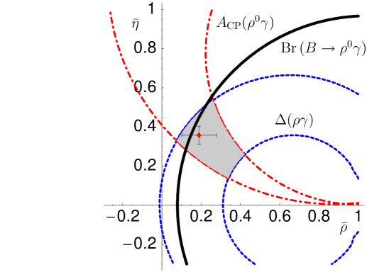
Figure 6: Constraints on the unitarity triangle from the ratio of the CP-averaged $B^{0}\to\rho^{0}\gamma$ and $B^{0}\to K^{*0}\gamma$ branching fractions (solid black), the isospin asymmetry in $B\to\rho\gamma$ (dashed) and the direct CP asymmetry in $B^{0}\to\rho^{0}\gamma$ (dash-dotted). The area to the left of the black line is excluded by the experimental limit on $B^{0}\to\rho^{0}\gamma$. See text for explanations.

No data currently exists for the isospin and direct CP asymmetries. To illustrate the possible constraints we assume that they are observed with a value that corresponds to our theoretical expectations (29,32) without experimental error. The theoretical uncertainty from the input parameters (excluding CKM parameters) then translates into the dashed (isospin asymmetry) and dash-dotted (direct CP asymmetry in $B\to\rho^{0}\gamma$) bands in the Figure. The constraint from the CP asymmetry in the charged decay $B^{\pm}\to\rho^{\pm}\gamma$ is very similar to the neutral one in the vicinity of the standard $(\bar{\rho},\bar{\eta})$ range and not shown. The shape of these constraints can be understood from the relations

$$R_{ut}\sin\alpha=\frac{\bar{\eta}}{(1-\bar{\rho})^{2}+\bar{\eta}^{2}},\qquad R_{ut}\cos\alpha=1-\frac{1-\bar{\rho}}{(1-\bar{\rho})^{2}+\bar{\eta}^{2}}.$$ (35)

They imply to good approximation that the direct CP asymmetry requires $(\bar{\rho},\bar{\eta})$ to lie on a circle of radius $1/(2a)$ with center $(1,1/(2a))$ where

$$a=\frac{A_{\rm CP}(\rho^{0}\gamma)}{2\epsilon_{0}\sin\theta_{0}},$$ (36)

which always passes through $(1,0)$. Similarly, the isospin asymmetry constrains $(\bar{\rho},\bar{\eta})$ to lie on a circle whose center is always at $\bar{\eta}=0$ and whose radius is determined from (29). We see from Figure 6 that the two asymmetry constraints intersect nearly orthogonally, the intersection region being shaded in grey. This area is further constrained by the limit on the $B\to\rho\gamma$ branching fraction. The three observables together (and a similar constraint from the direct asymmetry in $B^{\pm}\to\rho^{\pm}\gamma$) demonstrate that the $B\to\rho\gamma$ decays alone provide valuable independent information on CKM parameters. Furthermore, if inconsistencies with the standard CKM fit appeared, this would point towards anomalous effects in $b\to d\gamma$ transitions.

3.6 Forward-backward asymmetries

The forward-backward asymmetry in $B\to V\ell^{+}\ell^{-}$ decays is defined by

$$A_{\rm FB}(q^{2}) \equiv \frac{1}{d\Gamma/dq^{2}}\left(\,\int_{0}^{1}d(\cos\theta)\,\frac{d^{2}\Gamma}{dq^{2}d\cos\theta}-\int_{-1}^{0}d(\cos\theta)\,\frac{d^{2}\Gamma}{dq^{2}d\cos\theta}\right)$$ (37)

$$\propto \mbox{Re}\left({\cal C}_{9,\,\perp}^{(t)}(q^{2})-R_{ut}\,e^{\pm i\alpha}\,{\cal C}_{9,\,\perp}^{(u)}(q^{2})\right),$$

where the second line follows from (2.3). Note that we have not performed an average over CP-conjugate decays for the forward-backward asymmetry. The exponential reads $e^{-i\alpha}$ for $B$ decay, and $e^{i\alpha}$ for $\bar{B}$ decay.

The next-to-leading order prediction of the forward-backward asymmetry for the $B\to K^{*}\ell^{+}\ell^{-}$ decay has been discussed in detail in our previous paper [3]. For the $b\to s$ transitions the term ${\cal C}_{9,\,\perp}^{(u)}(q^{2})$ is negligible, because the corresponding $R_{ut}$ is very small. Hence there is no difference between $B$ and $\bar{B}$ decay, and the asymmetry zero is determined by the zero of the real part of ${\cal C}_{9,\,\perp}^{(t)}(q^{2})$. In [3] we found that the next-to-leading order correction shifts the zero by $30\%$, but once this correction is included, a precise measurement of the location of the zero translates into a determination of the Wilson coefficient $C_{9}$ with an accuracy of about $10\%$. Our updated result for the position of the forward-backward asymmetry zero reads

$$q_{0}^{2}[K^{*0}]=4.36^{+0.33}_{-0.31}\,\mbox{GeV}^{2},\qquad q_{0}^{2}[K^{*+}]=4.15^{+0.27}_{-0.27}\,\mbox{GeV}^{2}.\qquad$$ (38)

The small difference compared to [3] is due to the different treatment of form factors and the inclusion of isospin breaking power corrections in the present analysis.

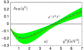
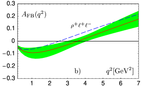
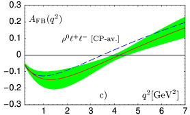
Figure 7: The forward-backward asymmetry in a) $B^{+}\to\rho^{+}\ell^{+}\ell^{-}$, b) $B^{-}\to\rho^{-}\ell^{+}\ell^{-}$, and c) the CP-averaged $B\to\rho^{0}\ell^{+}\ell^{-}$ decay. The solid (dashed) line shows the next-to-leading (leading) order result. The band represents the theoretical error due to hadronic uncertainties.

In case of $B\to\rho\,\ell^{+}\ell^{-}$ decays there exists an important new contribution from ${\cal C}_{9,\,\perp}^{(u)}(q^{2})$. As a consequence, the decays of $B$ or $\bar{B}$, neutral or charged $B$ mesons to $\rho\,\ell^{+}\ell^{-}$ may show significantly different forward-backward asymmetries. When $\alpha$ is near $90^{\circ}$ as expected in the Standard Model, we may approximate $e^{i\alpha}\simeq i\sin\alpha$, and therefore the additional contribution to the forward-backward asymmetry involves approximately

$$R_{ut}\sin\alpha\,{\rm Im}\,\Big{(}{\cal C}_{9\perp}^{(u)}(q^{2})\Big{)},$$ (39)

i.e. the absorptive part of the amplitude from the up-sector. We see from Table 5 that large contributions to the absorptive part arise from the virtual corrections to the $b\to d\ell^{+}\ell^{-}$ transition, $Y^{(u)}(q^{2})$ and $C^{(1)}$, and that, in particular, the two-loop correction $C^{(1)}$ calculated in [6, 7] is as large as the one-loop term $Y^{(u)}(q^{2})$. The other large contribution comes from weak annihilation and exists only for charged $B$ decays. In Figure 7 we show the expected forward-backward asymmetries for $B^{\pm}\to\rho^{\pm}\,\ell^{+}\ell^{-}$ and the asymmetry for the CP-averaged $B\to\rho^{0}\,\ell^{+}\ell^{-}$ decay rate. The locations of the asymmetry zeros are determined as

$$\begin{array}[]{cccc}&B^{0}\to\rho^{0}\,\ell^{+}\ell^{-}&\phantom{b}&\bar{B}^{0}\to\rho^{0}\,\ell^{+}\ell^{-}\\[5.69046pt] &4.34\,{}^{+0.02}_{-0.02}\big{|}_{\rm CKM}{}^{+0.45}_{-0.39}\big{|}_{\rm had}&&4.11\,{}^{+0.02}_{-0.02}\big{|}_{\rm CKM}{}^{+0.26}_{-0.22}\big{|}_{\rm had}\\[2.84544pt] q_{0}^{2}[\mbox{GeV}^{2}]\hskip 14.22636pt&&\\[-2.84544pt] &B^{+}\to\rho^{+}\,\ell^{+}\ell^{-}&&B^{-}\to\rho^{-}\,\ell^{+}\ell^{-}\\[5.69046pt] &3.56\,{}^{+0.09}_{-0.12}\big{|}_{\rm CKM}{}^{+0.48}_{-0.57}\big{|}_{\rm had}&&4.48\,{}^{+0.07}_{-0.06}\big{|}_{\rm CKM}{}^{+0.36}_{-0.34}\big{|}_{\rm had}\end{array}$$ (40)

As in the case of $B\to K^{*}\ell^{+}\ell^{-}$, the location of the asymmetry zero is a measure of $C_{9}$ (now in the $b\to d$ sector), but in addition information about the phase can be obtained through the interference with the tree-dominated amplitude in the up-sector.

4 Conclusions

Our analysis provides Standard Model expectations for the exclusive, radiative and electroweak penguin decays $B\to V\gamma$ and $B\to V\ell^{+}\ell^{-}$ ($V=K^{*},\rho,\omega$), extending our previous work [3] to $b\to d\gamma$ and $b\to d\ell^{+}\ell^{-}$ transitions. The theoretical framework is complete at next-to-leading order in the strong coupling (except for weak annihilation which is included only in leading order), and leading power in the heavy-quark expansion. We have also included $1/m_{b}$ power corrections, mainly from weak annihilation, which are important for the isospin asymmetries.

The observables related to $B\to\rho\gamma$ decays can provide interesting constraints on the CKM triangle as was also recently discussed in [15, 16]. The accuracy of these constraints is limited by hadronic uncertainties, mainly from the hadronic form factors describing the $B\to\rho$ transition (for branching fractions), $B\to\gamma$ transitions/weak annihilation (for the isospin asymmetry), and from the scale and charm quark mass uncertainty (for direct CP asymmetries). Nevertheless, the simultaneous measurement of branching fractions, isospin- and CP asymmetries can be used for an independent determination of the apex $(\bar{\rho},\bar{\eta})$ of the CKM triangle, which is complementary to the standard fit. In particular, if $B^{0}\to\rho^{0}\gamma$ is not observed with a branching fraction near the current upper limit $4\cdot 10^{-6}$, a tension with the standard fit arises.

We compared our calculations for $B\to K^{*}\ell^{+}\ell^{-}$ with the first experimental results on these decays. The central value of the Belle data on the partially integrated lepton invariant mass spectrum is about a factor of 2 larger than the theoretical prediction. Although the discrepancy is not significant within current uncertainties, it will be interesting to see how it develops. If the problem is theoretical, this may result in the curious situation that the comparison with data seems to favour a larger form factor $A_{0}$, but a smaller tensor form factor $T_{1}$. The present experimental accuracy for the measurement of the forward-backward lepton asymmetry in this decay mode is not yet competitive with the theoretical one. In the future, however, we expect significant constraints on the Wilson coefficient $C_{9}$ in $b\to s\ell^{+}\ell^{-}$ transitions as already discussed in [3].

We performed the first next-to-leading order calculation of exclusive $b\to d\ell^{+}\ell^{-}$ transitions. In the long run when detailed experimental information on these transitions will become available, the CKM matrix can be assumed to be known. Hence the various observables related to $B\to\rho\,\ell^{+}\ell^{-}$ decays provide information on the modulus and phase of the Wilson coefficient $C_{9}$ in $b\to d\ell^{+}\ell^{-}$ transitions or related coefficients in extended flavour models, which is of interest in the context of new-physics scenarios with non-minimal flavour violation. The theoretical uncertainty related to hadronic input is currently sizeable, but we may look forward to improved determinations of $B\to\rho$ form factors, and perhaps, the mechanism of weak annihilation, on the time scales of interest. These improvements will add $B\to\rho\,\ell^{+}\ell^{-}$ to the list of rare processes that play an essential role in the program to uncover the origin of flavour violation.

Acknowledgements

We would like to thank Patrick Koppenburg for helpful discussions, and Stefan Bosch for reading the manuscript. This work was supported by the DFG Sonderforschungsbereich/Transregio 9 “Computergestützte Theoretische Teilchenphysik”. M.B. would like to thank the INT, Seattle for its generous hospitality while part of the work was being done. D.S. acknowledges support of the DFG Graduiertenkolleg “Elementarteilchenphysik an der TeV-Skala” and would like to thank the CERN Theory group for hospitality.

Appendix A The amplitudes ${\cal T}_{a}^{(u,t)}$

In this appendix we present the generalization of the amplitudes ${\cal T}_{a}^{(t)}$ ($a=\perp,\parallel$) given in [3] for $B\to K^{*}\ell^{+}\ell^{-}$ to the case of $\rho$ or $\omega$ in the final state, and the new amplitudes ${\cal T}_{a}^{(u)}$ as defined in (3). In [3] we used a set of Wilson coefficients denoted by $\bar{C}_{i}$. The exact relation between the $\bar{C}_{i}$ and the $C_{i}$ given in Table 1 can be found in the appendix of [3].

The coefficient functions $C_{a}^{(i)}$ and $T^{(i)}_{a,\,\pm}$ defined in (4) have the expansions

$$C_{a}^{(i)} = C_{a}^{(0,i)}+\frac{\alpha_{s}C_{F}}{4\pi}\,C_{a}^{(1,i)}+\ldots,$$ (41)

$$T^{(i)}_{a,\,\pm}(u,\omega) = T^{(0,i)}_{a,\,\pm}(u,\omega)+\frac{\alpha_{s}C_{F}}{4\pi}\,T^{(1,i)}_{a,\,\pm}(u,\omega)+\ldots.$$ (42)

In the following we give the expressions for the coefficients $C_{a}^{(i)}$ and $T^{(i)}_{a,\,\pm}$. The strong coupling is evaluated at the scale $\mu\simeq m_{b}$ in (41) and at $\mu_{f}=(0.5\,\mbox{GeV}\mu)^{1/2}\simeq(m_{b}\Lambda_{\rm QCD})^{1/2}$ in (42), which corresponds to the typical virtualities in the two terms. In contrast to our earlier analysis, we always evaluate the Wilson coefficients at $\mu\simeq m_{b}$, since the running of the four-quark operators ends at this scale.

A.1 Form-factor term

The coefficients $C_{a}^{(0,t)}$ follow from Eqs. (12,14) in [3]. The corresponding expressions for $C_{a}^{(0,u)}$ are obtained by the replacements $C_{7}^{\rm eff}\to 0$ and

$$Y(s)\to Y^{(u)}(s)\equiv\left(\frac{4}{3}C_{1}+C_{2}\right)\left[h(s,m_{c})-h(s,0)\right],$$ (43)

where $h(s,m_{q})$ is given in Eq. (11) of [3].

The first-order corrections $C_{a}^{(1,i)}$ are divided into a “factorizable” and a “non-factorizable” term according to $C_{a}^{(1,i)}=C_{a}^{(f,i)}+C_{a}^{(nf,i)}$. The factorizable correction reads

$$C_{\perp}^{(f,t)} = C_{7}^{\rm eff}\left(\ln\frac{m_{b}^{2}}{\mu^{2}}-L+\Delta M\right),$$ (44)

$$C_{\parallel}^{(f,t)} = -C_{7}^{\rm eff}\left(\ln\frac{m_{b}^{2}}{\mu^{2}}+2L+\Delta M\right)$$ (45)

with $L$ defined in Eq. (36) of [3]. $\Delta M$ depends on the mass renormalization convention for the overall factor $m_{b}$ in (3), such that $\Delta M=0$ in the $\overline{\rm MS}$ scheme, $\Delta M=3\ln(m_{b}^{2}/\mu^{2})-4(1-\mu_{f}/m_{b})$ in the PS scheme (our choice) and $\Delta M=3\ln(m_{b}^{2}/\mu^{2})-4$ in the pole mass scheme. Note that the expression for $C_{\parallel}^{(f,t)}$ differs from Eq. (35) of [3] due to the different convention for the longitudinal “soft” form factor (5). Furthermore, when ${\cal T}^{(t)}_{\perp}$ is defined with $T_{1}$ rather than $\xi_{\perp}$, the corresponding $C_{\perp}^{(f,t)\prime}$ is given by (44) with the term $-L$ omitted. The factorizable corrections from $H_{\rm eff}^{(u)}$ follow again from $C_{7}^{\rm eff}\to 0$, which leads to $C_{\perp}^{(f,u)}=C_{\parallel}^{(f,u)}=0$.

The non-factorizable corrections $C_{a}^{(nf,t)}$ are given in Eqs. (37,38) of [3], and make use of the result from [36]. The corresponding expressions for $C_{a}^{(nf,u)}$ are obtained by the replacements $F_{8}^{(7,9)}\to 0$ and $F_{1,2}^{(7,9)}\to F_{1,2}^{(7,9)}+F_{1,2,u}^{(7,9)}$ with $F_{1,2,u}^{(7,9)}$ given in [6].

A.2 Spectator scattering

The longitudinal amplitude receives a leading-order contribution from a weak annihilation topology, where the photon couples to the spectator quark in the $B$ meson [3]. It is given by ($e_{q}$ denotes the charge of the spectator quark)

$$T_{\parallel,-}^{(0,t)}(u,\omega)=-e_{q}\,\frac{M_{B}\omega}{M_{B}\omega-q^{2}-i\epsilon}\,\frac{4M_{B}}{m_{b}}\,C_{q}^{34},$$ (46)

where

$$C_{q}^{34}\equiv C_{3}+\frac{4}{3}(C_{4}+12C_{5}+16C_{6})+6\,[1+(-1)^{I}]\,\delta_{qd}\,(C_{3}+10C_{5})$$ (47)

with $I=0,1$ for $\omega$ and $\rho$ mesons, respectively. The corresponding expression for $T_{\parallel,-}^{(0,u)}$ is obtained by the replacement $C_{q}^{34}\to-C_{q}^{12}$ with

$$C_{q}^{12}\equiv 3\,\delta_{qu}\,C_{2}+(-1)^{I}\,\delta_{qd}\,\left(\frac{4}{3}\,C_{1}+C_{2}\right).$$ (48)

The terms proportional to $\delta_{qd}$ in the previous two equations do not appear in $B\to K^{*}\ell^{+}\ell^{-}$ transitions. (Analogous terms with $\delta_{qd}\to\delta_{qs}$ would appear in $B_{s}\to\phi\ell^{+}\ell^{-}$.) There is no leading-order contribution from spectator scattering to $T_{\parallel,+}^{(0,i)}$ and the transverse amplitudes.

The first-order corrections are again divided into a “factorizable” and a “non-factorizable” term, $T_{a,\pm}^{(1,i)}=T_{a,\pm}^{(f,i)}+T_{a,\pm}^{(nf,i)}$. There is also a first-order correction to the annihilation mechanism discussed above, which is not yet known. $T_{\perp,\pm}^{(f,t)}$ and $T_{\parallel,-}^{(f,t)}$ are given in Eqs. (20,22) of [3], while now

$$T_{\parallel,+}^{(f,t)}=C_{7}^{\rm eff}\,\frac{4M_{B}}{\bar{u}E},$$ (49)

because of the different convention pertaining to the longitudinal “soft” form factor. The corresponding terms from $H_{\rm eff}^{(u)}$ all vanish, $T_{a,\pm}^{(f,u)}=0$. Furthermore, when ${\cal T}^{(t)}_{\perp}$ is defined with $T_{1}$ rather than $\xi_{\perp}$, the corresponding $T_{\perp,+}^{(f,t)\prime}$ is zero.

The non-factorizable amplitudes $T_{a,\pm}^{(nf,t)}$ are given in Eqs. (23-26) of [3]. The new amplitudes read

$$T_{\perp,+}^{(nf,u)}(u,\omega) = e_{u}\,\frac{M_{B}}{2m_{b}}\,\left(C_{2}-\frac{1}{6}C_{1}\right)\left(t_{\perp}(u,m_{c})-t_{\perp}(u,0)\right),$$

$$T_{\parallel,+}^{(nf,u)}(u,\omega) = e_{u}\,\frac{M_{B}}{m_{b}}\,\left(C_{2}-\frac{1}{6}C_{1}\right)\left(t_{\parallel}(u,m_{c})-t_{\parallel}(u,0)\right),$$

$$T_{\parallel,-}^{(nf,u)}(u,\omega) = e_{q}\,\frac{M_{B}\omega}{M_{B}\omega-q^{2}-i\epsilon}\,\frac{6M_{B}}{m_{b}}$$ (50)

$$\times\left(C_{2}-\frac{1}{6}C_{1}\right)\left(h(\bar{u}M_{B}^{2}+uq^{2},m_{c})-h(\bar{u}M_{B}^{2}+uq^{2},0)\right),$$

$T_{\perp,-}^{(nf,u)}(u,\omega)=0$, where the functions $t_{\perp,\parallel}(u,m)$ are defined in Eqs. (27,28) of [3].

A.3 Power-suppressed amplitudes

Some $1/m_{b}$-suppressed weak annihilation contributions play an important role in decays to charged $\rho$ mesons, because they are enhanced by the large Wilson coefficient $C_{2}$. In addition, power corrections may provide the dominant source of isospin breaking, since, as can be seen from the above formulae, the transverse amplitude is independent of the charge of the spectator quark in the leading order of the heavy quark expansion. On the contrary, all these effects are present in the longitudinal amplitude already at leading power. We therefore neglect power corrections to the longitudinal amplitude and summarize here the relevant expressions for isospin-breaking power corrections to the transverse amplitude.

Weak annihilation. Denoting the power-suppressed contributions to ${\cal T}_{\perp}^{(i)}$ defined in (4) by $\Delta{\cal T}_{\perp}^{(i)}$, we find for the annihilation terms at order $\alpha_{s}^{0}$ ($\hat{s}=q^{2}/M_{B}^{2}$)

$$\Delta{\cal T}_{\perp}^{(t)}\Big{|}_{\rm ann} = -e_{q}\,\frac{4\pi^{2}}{3}\,\frac{f_{B}f_{\perp}}{m_{b}M_{B}}\,\left(C_{3}+\frac{4}{3}(C_{4}+3C_{5}+4C_{6})\right)\,\int_{0}^{1}du\,\frac{\phi_{\perp}(u)}{\bar{u}+u\hat{s}}$$

$$+\,e_{q}\,\frac{2\pi^{2}}{3}\,\frac{f_{B}f_{\parallel}}{m_{b}M_{B}}\,\frac{m_{V}}{(1-\hat{s})\,\lambda_{B,+}(q^{2})}\,C_{q}^{34},$$

$$\Delta{\cal T}_{\perp}^{(u)}\Big{|}_{\rm ann} = -e_{q}\,\frac{2\pi^{2}}{3}\,\frac{f_{B}f_{\parallel}}{m_{b}M_{B}}\,\frac{m_{V}}{(1-\hat{s})\,\lambda_{B,+}(q^{2})}\,C_{q}^{12},$$ (51)

which generalizes the corresponding results in [31, 35]. The inverse moments of the $B$ meson distribution amplitudes, $\lambda_{B,\pm}(q^{2})$, are defined in Eq. (49,50) of [3].

Hard spectator scattering. The power-suppressed hard scattering terms at order $\alpha_{s}$ read [31, 35]

$$\Delta{\cal T}_{\perp}^{(t)}\Big{|}_{\rm hsa} = e_{q}\,\frac{\alpha_{s}C_{F}}{4\pi}\,\frac{\pi^{2}f_{B}}{N_{c}m_{b}M_{B}}\Bigg{\{}12C_{8}^{\rm eff}\,\frac{m_{b}}{M_{B}}\,f_{\perp}X_{\perp}(q^{2}/M_{B}^{2})$$ (52)

$$+\,8f_{\perp}\int_{0}^{1}du\,\frac{\phi_{\perp}(u)}{\bar{u}+u\hat{s}}\,F_{V}^{(t)}(\bar{u}M_{B}^{2}+uq^{2})$$

$$-\,\frac{4m_{V}f_{\parallel}}{(1-\hat{s})\,\lambda_{B,+}(q^{2})}\int_{0}^{1}du\int_{0}^{u}dv\,\frac{\phi_{\parallel}(v)}{\bar{v}}\,F_{V}^{(t)}(\bar{u}M_{B}^{2}+uq^{2})\Bigg{\}}.$$

The quark-loop function $F_{V}^{(t)}(s)$ is denoted $F_{V}(s)$ in [35], where also the integral $X_{\perp}(\hat{s})$ can be found. For $q^{2}=0$ this integral suffers from a logarithmic endpoint singularity as $u\to 1$. We treat this singularity, which signals a breakdown of factorization for the power corrections, with the same ad hoc cutoff as in [35]. The corresponding expression for $\Delta{\cal T}_{\perp}^{(u)}\Big{|}_{\rm hsa}$ is obtained by the replacements $C_{8}^{\rm eff}\to 0$ and $F_{V}^{(t)}(s)\to F_{V}^{(u)}(s)$, where

$$F_{V}^{(u)}(s)=\frac{3}{4}\left(C_{2}-\frac{1}{6}C_{1}\right)\,\big{[}h(s,m_{c})-h(s,0)\big{]}.$$ (53)

The numerically largest power correction is $\Delta{\cal T}_{\perp}^{(u)}\Big{|}_{\rm ann}$, because it comes with a large combination of Wilson coefficients $C_{q}^{12}\approx 3$ (when $q=u$, i.e. for $B^{\pm}$ decay). In this weak annihilation effect the photon is emitted from the spectator quark. Therefore the matrix element of ${\cal O}_{2}^{u}$ factorizes at leading order in $\alpha_{s}$ into

$$\langle\gamma^{*}(q,\mu)\rho^{-}(p^{\prime},\varepsilon^{*})|{\cal O}_{2}^{u}|B^{-}(p)\rangle=-if_{\rho}m_{\rho}\varepsilon^{*}_{\nu}\,\langle\gamma^{*}(q,\mu)|\bar{u}\gamma^{\nu}(1-\gamma_{5})b|B^{-}(p)\rangle$$ (54)

assuming the decay is $B^{-}\to\rho^{-}\ell^{+}\ell^{-}$, for which the effect is most important. The $B\to\gamma^{*}$ transition matrix element is dominated by hard scattering in the heavy quark limit, but power corrections (to weak annihilation, which is itself a power correction to the process of interest) may be significant, especially for $q^{2}\simeq 0$ [28, 29], where the hadronic structure of the photon may be resolved. To keep the discussion general, we parameterize the matrix element by

$$\langle\gamma^{*}(q,\mu)|\bar{u}\gamma^{\nu}(1-\gamma_{5})b|B^{-}(p)\rangle = ig_{\rm em}e_{q}\,\frac{M_{B}}{2}\bigg{\{}\xi_{\perp}^{(B\gamma^{*})}(q^{2})\left[i\,\epsilon^{\mu\nu\rho\sigma}n_{+\rho}n_{-\sigma}+2g_{\perp}^{\mu\nu}\right]$$ (55)

$$-\,2\,\xi_{\parallel}^{(B\gamma^{*})}(q^{2})\,n_{+}^{\mu}n_{+}^{\nu}\bigg{\}}+\mbox{corrections},$$

where the vectors $n_{\pm}$ are given by $p^{\prime}=En_{-}$ ($E$ the energy of the $\rho$ meson) and $p=M_{B}(n_{-}+n_{+})/2$. The form factors defined by this parameterization describe the transition of a $B$ meson into a virtual photon of mass $\sqrt{q^{2}}$ at zero momentum transfer $p^{\prime\,2}=(p-q)^{2}=0$. In the heavy quark limit we find

$$\xi_{\perp}^{(B\gamma^{*})}(q^{2})=\frac{f_{B}}{2\lambda_{B+}(q^{2})},\qquad\xi_{\parallel}^{(B\gamma^{*})}(q^{2})=\frac{f_{B}}{2\lambda_{B-}(q^{2})}.$$ (56)

The “corrections” stand for additional Lorentz structures that vanish in the heavy quark limit, and also when the leading corrections from the hadronic structure of the photon are included. We may therefore adopt a more conservative treatment of the leading weak annihilation effects by expressing (46) (and, accordingly, $T_{\parallel,-}^{(0,u)}$) in terms of $\xi_{\parallel}^{(B\gamma^{*})}(q^{2})$ and (51) in terms of $\xi_{\perp}^{(B\gamma^{*})}(q^{2})$. The transverse form factor at $q^{2}=0$ has been estimated with QCD sum rules [28, 29], leading to a result not too different from the heavy quark limit (56). In our numerical analysis we use (56) to compute the central value of these form factors, but we assign a 50% theoretical error to this estimate.

References

- [1] M. Beneke, G. Buchalla, M. Neubert and C. T. Sachrajda, Phys. Rev. Lett. 83 (1999) 1914 [hep-ph/9905312].
- [2] M. Beneke, G. Buchalla, M. Neubert and C. T. Sachrajda, Nucl. Phys. B 591 (2000) 313 [hep-ph/0006124].
- [3] M. Beneke, T. Feldmann and D. Seidel, Nucl. Phys. B 612 (2001) 25 [hep-ph/0106067].
- [4] S. W. Bosch and G. Buchalla, Nucl. Phys. B 621 (2002) 459 [hep-ph/0106081].
- [5] A. Ali and A. Y. Parkhomenko, Eur. Phys. J. C 23 (2002) 89 [hep-ph/0105302].
- [6] D. Seidel, Phys. Rev. D 70 (2004) 094038 [hep-ph/0403185].
- [7] H. M. Asatrian, K. Bieri, C. Greub and M. Walker, Phys. Rev. D 69 (2004) 074007 [hep-ph/0312063].
- [8] J. g. Chay and C. Kim, Phys. Rev. D 68 (2003) 034013 [hep-ph/0305033].
- [9] S. Descotes-Genon and C. T. Sachrajda, Nucl. Phys. B 693 (2004) 103 [hep-ph/0403277].
- [10] B. Aubert et al. [BABAR Collaboration], [hep-ex/0408034].
- [11] K. Abe et al. [BELLE Collaboration], [hep-ex/0408137].
- [12] B. Aubert et al. [BABAR Collaboration], Phys. Rev. Lett. 91 (2003) 221802 [hep-ex/0308042].
- [13] A. Ishikawa et al. [Belle Collaboration], Phys. Rev. Lett. 91 (2003) 261601 [hep-ex/0308044].
- [14] K. Abe et al. [Belle Collaboration], [hep-ex/0410006].
- [15] A. Ali, E. Lunghi and A. Y. Parkhomenko, [hep-ph/0405075].
- [16] S. W. Bosch and G. Buchalla, [hep-ph/0408231].
- [17] P. Gambino, M. Gorbahn and U. Haisch, Nucl. Phys. B 673 (2003) 238 [hep-ph/0306079].
- [18] M. Gorbahn and U. Haisch, [hep-ph/0411071].
- [19] M. Beneke and T. Feldmann, Nucl. Phys. B 592 (2001) 3 [hep-ph/0008255].
- [20] J. Charles et al., [hep-ph/0406184].
- [21] M. Beneke, Phys. Lett. B 434 (1998) 115 [hep-ph/9804241].
- [22] V. M. Braun, D. Y. Ivanov and G. P. Korchemsky, Phys. Rev. D 69 (2004) 034014 [hep-ph/0309330].
- [23] M. Beneke and M. Neubert, Nucl. Phys. B 675 (2003) 333 [hep-ph/0308039].
- [24] A. Khodjamirian, T. Mannel and M. Melcher, [hep-ph/0407226].
- [25] V. M. Braun and A. Lenz, [hep-ph/0407282].
- [26] P. Ball and V. M. Braun, Phys. Rev. D 58 (1998) 094016 [hep-ph/9805422].
- [27] C. Greub, T. Hurth and D. Wyler, Phys. Rev. D 54 (1996) 3350 [hep-ph/9603404].
- [28] A. Khodjamirian, G. Stoll and D. Wyler, Phys. Lett. B 358 (1995) 129 [hep-ph/9506242].
- [29] A. Ali and V. M. Braun, Phys. Lett. B 359 (1995) 223 [hep-ph/9506248].
- [30] B. Grinstein and D. Pirjol, Phys. Rev. D 62 (2000) 093002 [hep-ph/0002216].
- [31] A. L. Kagan and M. Neubert, Phys. Lett. B 539 (2002) 227 [hep-ph/0110078].
- [32] B. Aubert et al. [BABAR Collaboration], [hep-ex/0407003].
- [33] M. Nakao et al. [BELLE Colaboration Collaboration], [hep-ex/0402042].
- [34] T. E. Coan et al. [CLEO Collaboration], Phys. Rev. Lett. 84 (2000) 5283 [hep-ex/9912057].
- [35] T. Feldmann and J. Matias, JHEP 0301 (2003) 074 [hep-ph/0212158].
- [36] H. H. Asatryan, H. M. Asatrian, C. Greub and M. Walker, Phys. Rev. D 65 (2002) 074004 [hep-ph/0109140].