The radiative decays $\phi\to\gamma a_{0}/f_{0}$ in the molecular model for the scalar mesons

Abstract

We investigate the radiative decays of the $\phi$ meson to the scalar mesons $a_{0}(980)$ and $f_{0}(980)$. We demonstrate that, contrary to earlier claims, these decays should be of the same order of magnitude for a molecular state and for a compact state and, therefore, the available experimental information is consistent with both, a molecular as well as a compact structure of the scalars. Thus, the radiative decays of the $\phi$ meson into scalars establish a sizable $K\bar{K}$ component of the scalar mesons, but do not allow to discriminate between molecules and compact states.

1 Introduction

It has been claimed for many years that studies of radiative decays $\phi\to\gamma a_{0}(980)\to\gamma\pi^{0}\eta$ and $\phi\to\gamma f_{0}(980)\to\gamma\pi^{0}\pi^{0}$ are a powerful tool to discriminate between various models for the low-lying scalar mesons. The extraction of the $\phi\gamma a_{0}$ and $\phi\gamma f_{0}$ coupling constants from the data is not a straightforward task (see Pennington ), but it is a common belief that, with data accurate enough, radiative decays would reveal the nature of the lightest scalars.

The simplest mechanism for these radiative decays assumes that the $a_{0}$ and $f_{0}$ are ${}^{3}P_{0}$ quarkonia, and the decays proceed via a quark loop. Nevertheless, with the $\phi$-meson being mostly an $s\bar{s}$ state, this mechanism cannot be responsible for the decay $\phi\to\gamma a_{0}$, since, in the quarkonium picture, the $a_{0}$ is an isovector state made of light quarks. Similarly, only $f_{0}(s\bar{s})$ can be produced via the quark loop mechanism and, if so, the subsequent decay $f_{0}\to\pi^{0}\pi^{0}$ is suppressed by the OZI rule. On the other hand, as both $f_{0}$ and $a_{0}$ are close to the $K\bar{K}$ threshold and are known to couple strongly to this channel, one expects that the radiative decay mechanism via charged kaon loop should play an essential role, as it was suggested in Refs. AI ; CIK ; AGS . The existing data on $\phi$ radiative decays SND ; CMD ; KLOE support this expectation, as is shown in detail in Ref. Achasov .

The latter observation does not mean per se that the quarkonium assignment for $a_{0}$ and $f_{0}$ is excluded by the data. It only means that the strong coupling to the $K\bar{K}$ channel, together with the threshold enhancement phenomenon, makes the kaon loop mechanism dominant. However, the strong coupling to $K\bar{K}$ implies that the $K\bar{K}$ component in the wave functions of these mesons should be large, and recent studies W based on the analysis of near-threshold data confirm this. A large $K\bar{K}$ admixture should be reflected somehow in the radiative decay amplitude.

In Ref. CIK it is claimed that there should be a strong suppression of the $\phi\to\gamma f_{0}/a_{0}$ branching ratio for the scalars in case they are loosely bound molecules as compared to pointlike scalars that correspond to compact quark states, ($10^{-5}$ vs $10^{-4}$). A study by Achasov et al. AGS , where the finite width of scalars was taken into account, arrived at the same conclusion. Thus, the authors of CIK and AGS stress that data for this branching ratio should allow to prove or rule out the molecular model of the scalars. However, no such suppression was found in recent kaon loop calculations, Refs. Oset ; Markushin ; Oller , where the scalars were considered as dynamically generated states, i.e., as molecules. The aim of the present paper is to demonstrate explicitly the implications of a molecular structure of scalars on the radiative $\phi$ decay. In the course of this we can demonstrate what went wrong in the analysis of Ref. CIK and confirm the results of Refs. Oset ; Markushin ; Oller .

2 Point–like scalars

To simplify the situation we work with stable scalars — the generalization to a more realistic case is straight forward and should not change the conclusions; we comment on what is necessary for this generalization in what follows. The current describing the radiative transition between the vector meson $\phi$ and a scalar meson $S$, in the kaon loop model, is written as Nussinov ; Lucio (see CIK for notations)

$$M_{\nu}=e\frac{g_{\phi}g_{S}}{2\pi^{2}im^{2}_{K}}I(a,b)[\varepsilon_{\nu}(p\cdot q)-p_{\nu}(q\cdot\varepsilon)],$$ (1)

where $p$ and $q$ are the momenta of the $\phi$-meson and the photon, respectively, $m_{K}$ is the kaon mass, $g_{\phi}$ and $g_{S}$ are the $\phi K^{+}K^{-}$ and $SK^{+}K^{-}$ coupling constants, $\varepsilon_{\nu}$ is the polarization four-vector of the $\phi$-meson, $a=\frac{m^{2}_{\phi}}{m^{2}_{K}}$, and $b=\frac{m^{2}_{S}}{m^{2}_{K}}$ (in case of an unstable particle produced $m^{2}_{S}$ is to be replaced by the invariant mass squared of the decay products). The amplitude (1) is transverse, $M_{\nu}q_{\nu}=0$, and is proportional to the photon momentum.

For the pointlike model of the scalar mesons the function $I(a,b)$ was calculated in Refs. AI ; CIK . It is given by

$$I(a,b)=\frac{1}{2(a-b)}-\frac{2}{(a-b)^{2}}\left[f\left(\frac{1}{b}\right)-f\left(\frac{1}{a}\right)\right]+\frac{a}{(a-b)^{2}}\left[g\left(\frac{1}{b}\right)-g\left(\frac{1}{a}\right)\right],$$ (2)

$$f(\alpha)=\left\{\begin{array}[]{ccc}-[\arcsin(\frac{1}{2\sqrt{\alpha}})]^{2},&&\alpha>\frac{1}{4}\\ \frac{1}{4}\left[\ln(\frac{\eta_{+}}{\eta_{-}})-i\pi\right],&&\alpha<\frac{1}{4}\end{array}\right.$$

$$g(\alpha)=\left\{\begin{array}[]{ccc}\sqrt{4\alpha-1}\arcsin(\frac{1}{2\sqrt{\alpha}}),&&\alpha>\frac{1}{4}\\ \frac{1}{2}\sqrt{1-4\alpha}\left[\ln(\frac{\eta_{+}}{\eta_{-}})-i\pi\right],&&\alpha<\frac{1}{4}\end{array}\right.$$

$$\eta_{\pm}=\frac{1}{2\alpha}\left(1\pm\sqrt{1-4\alpha}\right).$$

Note that the integral $I(a,b)$ remains finite in the limit $a\to b$.

To arrive at the formula (1) consider the sum of the graphs depicted in Fig. 1(a)-(c), where the appearance of the graph 1(c) is a consequence of gauge invariance, since the $\phi\to K\bar{K}$ vertex is momentum-dependent. The current in Eq. (1) is given by $M_{\nu}=eg_{\phi}g_{S}\varepsilon_{\mu}J_{\mu\nu}$, with

$$J_{\mu\nu}=J^{(a)}_{\mu\nu}+J^{(b)}_{\mu\nu}+J^{(c)}_{\mu\nu}=2J^{(a)}_{\mu\nu}+J^{(c)}_{\mu\nu},$$ (3)

where

$$J^{(a)}_{\mu\nu}=\int\frac{d^{4}k}{(2\pi)^{4}}\frac{(2k-p)_{\mu}(2k-q)_{\nu}}{[k^{2}-m^{2}+i0][(k-q)^{2}-m^{2}+i0][(k-p)^{2}-m^{2}+i0]},$$ (4)

$$J^{(c)}_{\mu\nu}=-2g_{\mu\nu}\int\frac{d^{4}k}{(2\pi)^{4}}\frac{1}{[k^{2}-m^{2}+i0][(q+k-p)^{2}-m^{2}+i0]},$$ (5)

and $m=m_{K}$.

(a)	(b)	(c)	(d)

Figure 1: Diagrams contributing to the radiative decay amplitude (1).

Since gauge invariance demands the structure of the integral (3) to be

$$J_{\mu\nu}=J[p_{\nu}q_{\mu}-(p\cdot q)g_{\mu\nu}],$$ (6)

the strategy applied in Ref. CIK is to read off the coefficient of the $p_{\nu}q_{\mu}$ term, coming entirely from the integral (4), and to restore then the coefficient of the $g_{\mu\nu}$ term with the help of Eq. (6). This allows the authors to deal with a finite integral and thus to bypass the problem of treating the divergent parts of the loop integrals (4), (5). However, as we shall see below, the divergent pieces cancel and the sum of diagrams given in Eq. (3) is finite Bramon .

To see this we decompose the expression for $J_{\mu\nu}^{(a)}$ as

$$2J^{(a)}_{\mu\nu}=J[p_{\nu}q_{\mu}-(p\cdot q)g_{\mu\nu}]+2g_{\mu\nu}J^{\prime}_{a}\ ,$$ (7)

where

$$J=-\frac{i}{2\pi^{2}m^{2}}\left\{\frac{1}{(a-b)}\int^{1}_{0}dz\left[1-z-\frac{1-az(1-z)}{z(a-b)}\ln\frac{1-bz(1-z)}{1-az(1-z)}\right]\right.$$ (8)

$$\hskip 85.35826pt\left.-\frac{i\pi}{(a-b)^{2}}\int^{1/\eta_{+}}_{1/\eta_{-}}dz\left[\frac{1}{z}-(1-z)a\right]\right\}=-\frac{i}{\pi^{2}m^{2}}I(a,b).$$

Here and in what follows we consider the case of $m_{\phi}>2m$, $m_{S}<2m$. In addition

$$J^{\prime}_{a}=\frac{i}{16\pi^{2}}\left[\frac{2}{\varepsilon}-\gamma_{E}-\ln\frac{m^{2}}{4\pi\mu_{\varepsilon}^{2}}\right]-\frac{i}{8\pi^{2}}\int^{1}_{0}dz(1-z)\ln[1-bz(1-z)],$$ (9)

where $\mu_{\varepsilon}$ is the auxiliary mass parameter, the number of dimensions $D$ is equal to $4-\varepsilon$, and $\gamma_{E}$ is the Euler constant. Similarly, the contact term (5) can be presented as $-2g_{\mu\nu}J^{\prime}_{c}$ with

$$J^{\prime}_{c}=\frac{i}{16\pi^{2}}\left[\frac{2}{\varepsilon}-\gamma_{E}-\ln\frac{m^{2}}{4\pi\mu_{\varepsilon}^{2}}\right]-\frac{i}{16\pi^{2}}\int^{1}_{0}dz\ln[1-bz(1-z)],$$ (10)

and, since

$$\int^{1}_{0}dz(1-2z)\ln[1-bz(1-z)]=0,$$

the structure (6) is restored. We conclude therefore that, with the proper regularization, the total matrix element is finite. It means that the range of convergence of the integrals involved is defined only by the kinematics of the problem. In particular, if both masses of the vector and scalar mesons are close to the $K\bar{K}$ threshold, the integrals converge at $k_{0}\sim m$ and for nonrelativistic values of the three-dimensional loop momentum ${\rm k}$, $|\mbox{\boldmath${\rm k}$}|\ll m$. The nonrelativistic limit of the integral $I(a,b)$ takes the form

$$I_{NR}(a,b)=\frac{\pi(x^{3}+3xy^{2})}{24(x^{2}+y^{2})^{2}}+i\frac{\pi y^{3}}{12(x^{2}+y^{2})^{2}},$$ (11)

where

$$y=\sqrt{(a/4)-1}\,\quad x=\sqrt{1-(b/4)}\,,\quad x,y\ll 1.$$

Note that, although the expression (11) contains the factor $\frac{1}{x^{2}+y^{2}}\sim\frac{1}{a-b}$, it does not mean that $I_{NR}(a,b)$ blows up in the limit of zero photon energy, $\omega\rightarrow 0$. Indeed, the formula (11) is valid for the scalar meson lying below the $K\bar{K}$ threshold, so one cannot put $\omega=0$ here. If the scalar appears above the kaon threshold, Eq. (11) is replaced by

$$\frac{\pi i}{24}\frac{(2y+\tilde{x})}{(y+\tilde{x})^{2}},\quad\tilde{x}=\sqrt{(b/4)-1}$$ (12)

so that $I(a,b)$ remains finite in the limit $\omega\to 0$.

3 Introducing the scalar wave function

When treating the scalar meson as an extended (non-pointlike) object it is not sufficient to insert the corresponding form factor into the $K^{+}K^{-}S$ vertex (see CIK ), but gauge invariance calls for a correction term induced by this additional flow of charge. Since only soft photons are involved the needed correction term can be expressed as the derivative of the formfactor inserted. Thus we get for the induced vertex

$$\Gamma_{\nu}(K^{+}K^{-}S\gamma)=-2(p^{+}_{\nu}-p^{-}_{\nu})\left.\frac{\partial\Gamma(p^{2},m^{2})}{\partial p^{2}}\right|_{p^{2}=m^{2}},$$ (13)

where $\Gamma(p_{+}^{2},p_{-}^{2})=\Gamma(p_{-}^{2},p_{+}^{2})$ parameterizes the momentum dependence of the $K^{+}K^{-}S$ vertex, with $\Gamma(m^{2},m^{2})=1$. Here $p^{+}_{\nu}$ and $p^{-}_{\nu}$ are the $K^{+}$ and $K^{-}$ four-momenta, respectively. The corresponding extra diagram is depicted at Fig 1(d).

Before proceeding further we note that inclusion of the extra contact vertex (13) is a way to insert an ultraviolet cutoff in a gauge invariant way. As demonstrated above, the integrals of interest converge already for nonrelativistic momenta even for a pointlike vertex, thus it is justified to use nonrelativistic kinematics also when the vertex function $\Gamma$ is included, as it was done in Markushin — one only needs the mild assumption that $\Gamma$ decreases faster than $1/k$ for increasing values of its arguments. Then only the positive-energy parts of the kaon propagators are retained, the kaon energies are replaced by $m$, and $m_{\phi}$ and $m_{S}$ are replaced by $2m$, wherever possible. As to the vertex function, in the nonrelativistic description the virtuality of kaons is measured by the relative momentum of kaons in the intermediate state, so that in the center-of-mass frame of the vector meson ($\vec{p}=0$) the vertex function $\Gamma$ is a function of the three-momentum of the outgoing kaons only and thus the spatial loop integrals read

$$J_{ik}=2J^{(a)}_{ik}+J^{(c)}_{ik}+J^{(d)}_{ik}=-\delta_{ik}\frac{i}{4\pi^{2}}(a-b)I(a,b;\Gamma)+...~{},$$ (14)

when evaluated in the rest frame of the vector meson. Terms that do not contribute to the process of interest are not shown explicitly. Note, gauge invariance is enshured by the appearance of the term $(a-b)$ that vanishes for vanishing outgoing photon energy. The individual integrals are

$$2J^{(a)}_{ik} = -\frac{i}{m^{3}}\int\frac{d^{3}k}{(2\pi)^{3}}\frac{k_{i}k_{k}\Gamma(|\mbox{\boldmath${\rm k}$}-\mbox{\boldmath${\rm q}$}/2|)}{[E_{V}-\frac{k^{2}}{m}+i0][E_{S}-\frac{(\mbox{\boldmath${\rm k}$}-\mbox{\boldmath${\rm q}$}/2)^{2}}{m}+i0]},$$

$$J^{(c)}_{ik} = -\frac{i}{2m^{2}}\delta_{ik}\int\frac{d^{3}k}{(2\pi)^{3}}\frac{\Gamma(k)}{E_{S}-\frac{k^{2}}{m}+i0},$$

$$J^{(d)}_{ik} = -\frac{i}{2m^{2}}\int\frac{d^{3}k}{(2\pi)^{3}}\frac{k_{i}k_{k}}{E_{V}-\frac{k^{2}}{m}+i0}\frac{1}{k}\frac{\partial\Gamma(k)}{\partial k},$$ (15)

We assume $E_{V}=m_{V}-2m>0$, $E_{S}=m_{S}-2m<0$ for looking at only one kinematic regime is sufficient to make our point clear. For more realistic calculations that include the finite width of the scalar mesons we recommend Refs. Oset ; Markushin ; Oller . Performing integration by parts in the integral $J^{(d)}_{ik}$, one has

$$J^{(d)}_{ik}=\frac{i}{2m^{2}}\delta_{ik}\int\frac{d^{3}k}{(2\pi)^{3}}\frac{\Gamma(k)}{E_{V}-\frac{k^{2}}{m}+i0}+\frac{i}{3m^{3}}\delta_{ik}\int\frac{d^{3}k}{(2\pi)^{3}}\frac{k^{2}\Gamma(k)}{(E_{V}-\frac{k^{2}}{m}+i0)^{2}}.$$ (16)

This trick was used both in Refs. CIK and Markushin .

Let us now assume that $\Gamma$ decreases with the range $\beta$ that satisfies the conditions

$$\beta^{2}\gg mE_{V},\quad\beta^{2}\gg m|E_{S}|.$$ (17)

With the help of the representation (16) one immediately sees that, in the limit $\beta\rightarrow\infty$, the divergent terms in $J_{ik}$, Eq. (14), cancel each other and, in the leading nonrelativistic approximation, $E_{V}\ll m$, $|E_{S}|\ll m$, the total matrix element does not depend on $\beta$:

$$I(a,b;\Gamma)=I_{NR}(a,b).$$ (18)

We stress that the result (18) follows from the nonrelativistic formula (14), and the only condition needed is (17).

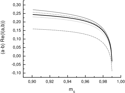
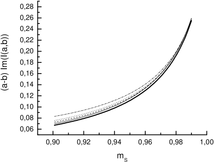
We have repeated the calculation of $I(a,b;\Gamma)$ presented in Ref. Markushin with the model form factor $\Gamma(\mbox{\boldmath${\rm k}$})=\beta^{2}/(\mbox{\boldmath${\rm k}$}^{2}+\beta^{2})$. The results are depicted at Fig. 2 together with the results of the full pointlike theory. One can see that, in the soft-photon limit, there is no considerable suppression of the matrix element due to finite values of $\beta$, down to $\beta\sim 0.3$ GeV. The reason for this was discussed above — the integral of Eq. (3) converges for nonrelativistic values of $|\mbox{\boldmath${\rm k}$}|$, in the soft-photon limit.

   

Figure 2: The real (the left plot) and the imaginary (the right plot) parts of the function $I_{1}=(a-b)I(a,b;\Gamma)$ for $\beta=0.2$ GeV (dash-dotted line), $\beta=0.4$ GeV (dotted line), $\beta=0.6$ GeV (dashed line), and $\beta=0.8$ GeV (thin solid line). The result of the full pointlike theory is given by the thick solid line.

Now we specify the form factor in the molecular model for the scalar mesons. To this end we use the well-known quantum–mechanical expressions which relate the $K\bar{K}S$ vertex and the wave function of the molecule. In the vicinity of a bound state the nonrelativistic $t$-matrix $t(\mbox{\boldmath${\rm k}$},\mbox{\boldmath${\rm k}$}^{\prime},E)$ takes the form

$$t(\mbox{\boldmath${\rm k}$},\mbox{\boldmath${\rm k}$}^{\prime},E)=\frac{\gamma(\mbox{\boldmath${\rm k}$})\gamma(\mbox{\boldmath${\rm k}$}^{\prime})}{E+\varepsilon-i0},\quad\gamma(\mbox{\boldmath${\rm k}$})=\hat{v}\phi(\mbox{\boldmath${\rm k}$}),$$ (19)

where $\phi(\mbox{\boldmath${\rm k}$})$ is the bound–state wave function in the momentum space, normalized to unity, $\varepsilon=-E_{S}$ is the binding energy, and the Schrödinger equation for the bound state is written symbolically as

$$\frac{\mbox{\boldmath${\rm k}$}^{2}}{m}\phi(\mbox{\boldmath${\rm k}$})+\hat{v}\phi(\mbox{\boldmath${\rm k}$})=-\varepsilon\phi(\mbox{\boldmath${\rm k}$}).$$ (20)

The relativistic vertex differs from the nonrelativistic vertex $\gamma$ by a kinematical factor (see, e.g., Landau ),

$$g_{S}\Gamma(\mbox{\boldmath${\rm k}$})=(2\pi)^{3/2}\sqrt{8m^{2}m_{S}}\;\gamma(\mbox{\boldmath${\rm k}$}),$$ (21)

where the effective coupling $g_{S}$ is introduced to ensure the normalization condition $\Gamma(0)=1$. Using the bound–state equation (20), one has, finally,

$$g_{S}\Gamma(\mbox{\boldmath${\rm k}$})=(2\pi)^{3/2}\sqrt{8m^{2}m_{S}}\left(\frac{\mbox{\boldmath${\rm k}$}^{2}}{m}+\varepsilon\right)\phi(\mbox{\boldmath${\rm k}$}).$$ (22)

Thus we find that the momentum dependent factor that appears in Eq. (22) exactly compensates for the two kaon propagator in Eq. (15). The wavefunction then supplies exactly that piece due to its demanded asymptotics.

A real molecule is a loosely bound state with a large mean distance between the constituents — much larger than the range of the binding force $r_{0}$. In this deuteronlike case one has

$$\phi(\mbox{\boldmath${\rm k}$})=\frac{\sqrt{\kappa}}{\pi}\frac{1}{\mbox{\boldmath${\rm k}$}^{2}+\kappa^{2}},\quad\kappa=\sqrt{m\varepsilon}.$$ (23)

Correspondingly, the vertex (22) does not depend on ${\rm k}$, and one can safely use the formulae (1), (2) of the pointlike theory with

$$g_{S}=\frac{(2\pi)^{3/2}}{\pi}\sqrt{8m_{S}\kappa},\quad\frac{g_{S}^{2}}{4\pi}\approx 32m\sqrt{m\varepsilon}.$$ (24)

The nonrelativistic expansion (11) of the integral $I(a,b)$ can be used as well.

So we conclude that the range $\beta$ of the form factor should be identified with the inverse range of the force, $\beta\sim 1/r_{0}$, and, if the inequality

$$\kappa r_{0}\sim\frac{\kappa}{\beta}\ll 1$$ (25)

holds true, the results of the pointlike theory for the radiative $\phi\to\gamma S$ decay are valid for molecular model of the scalar. In particular, there is no special suppression of the matrix element due to a finite value of $\beta$.

The latter statement is based on the validity of the inequality (25). What values of $\beta$ would one expect in realistic models of the $K\bar{K}$ molecule? In the meson-exchange models like Jue it is argued that a strong $t$-channel force is responsible for the formation of scalars. In such a case it is reasonable to identify $\beta$ with the mass of the lightest meson exchanged. As there is no pion exchange in the scalar sector, the lightest meson should be the $\rho$, which gives for $\beta$ the value of about $0.8$ GeV. In the phenomenological picture of Ref. Markushin , $\beta$ is taken to be $0.5\div 0.7$ GeV. In the quark language, $\beta$ is defined by the scale of the internal size of the quark wave function, which also leads to the estimate for $\beta$ to be of the order of a few hundred MeV. With such estimates, the inequality (25) is safely valid for the masses of the scalar about $970\div 980$ MeV.

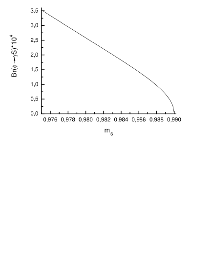
The formula (24) implies that the vertex $g_{S}$ depends on the binding energy and its value decreases with decreasing binding energy. This in turn causes a suppression of the branching ratio when the binding energy tends to zero, cf. Fig. 3. However, for binding energies of typical order of magnitude, for example, $\varepsilon=10$ MeV, Eq. (24) yields a coupling constant $g_{S}$ of

$$\frac{g_{S}^{2}}{4\pi}=1.12\ GeV^{2}.$$ (26)

That corresponds to a branching ratio of $Br(\phi\to\gamma S)\approx 2.6\times 10^{-4}$ which means that there is practically no suppression.

Nevertheless, we should emphasize in this context that a reliable quantitative calculation of the width certainly requires a more realistic approach where it is taken into account that the scalar mesons have finite widths due to the presence of the light pseudoscalar channels, and that the quantities that are really measured are the transitions $\phi\to\gamma\pi\pi$ or $\phi\to\gamma\pi\eta$. The impact of finite width effects have been thoroughly investigated by J.A. Oller Oller and also by Achasov and Gubin Gubin and we refer to their work for details. Here we only want to make the reader aware of the fact that due to the proximity of the $\gamma S$ threshold to the mass of the $\phi(1020)$ resonance even small variations in the nominal resonance masses of the scalar mesons have a drastic effect on the available phase space and in turn on the obtained results – as it can be imagined from Fig. 3 – unless the finite width of the ($f_{0}(980)$ or $a_{0}(980)$) scalar mesons is considered Oller ; Gubin .

To take into account finite width effects one has to use the two-channel version of Eq. (19) from the very beginning so that the vertex which appears in the loop integral is accompanied by the vertex that appears in the resonance decay, as it is required by the two-channel unitarity condition. If the characteristic scale $\beta$ in this full $t$-matrix is not too small, then the feature that there is no specific suppression due to the molecular structure of the scalar mesons will be preserved, cf. appendix A.

Figure 3: The dependence of the branching $Br(\phi\to\gamma S)$ on the mass of the scalar meson in the molecular model.

4 Comparison to older work and conclusions

Our findings are in contradiction with the results of Ref. CIK . The specific model for the $K\bar{K}$ molecule used there was taken from Ref. Barnes , which, in turn, is a modification of the approach developed in Ref. Isgur and based on the quark–exchange picture. The $K\bar{K}$ interaction employed in Ref. Barnes was approximated by a local potential of the form

$$V(r)=-V_{0}\exp{\left[-\frac{1}{2}\left(\frac{r}{r_{0}}\right)^{2}\right]},$$ (27)

with $r_{0}=0.57$ fm. This interaction gives $\varepsilon=10$ MeV, so that $\kappa r_{0}\sim 0.2$, and the molecule is rather deuteronlike.

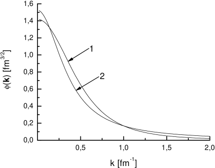
The wave function was parameterized as

$$\psi(r)=\left(\frac{\mu^{3}}{\pi}\right)^{1/2}e^{-\mu r},\quad\phi(\mbox{\boldmath${\rm k}$})=\frac{(2\mu)^{3/2}}{\pi}\frac{\mu}{(\mbox{\boldmath${\rm k}$}^{2}+\mu^{2})^{2}},$$ (28)

with $\mu=0.144$ GeV. This wave function yields a good approximation for the exact wave function, in the momentum space (see CIK ). On the other hand, the wave function (23) with $\varepsilon=10$ MeV looks very similar, see Fig. 4.

Figure 4: The wave function of the $K\bar{K}$ system, in momentum space. The approximate solution Eq. (28) — the curve 1, and the deuteronlike wave function, Eq. (23) — the curve 2.

So what is wrong with Ref. CIK , and where does the suppression of the radiative decay amplitude come from? The answer is rather simple. In Ref. CIK , the calculations of the loop integrals were performed with using the wave function

$$\phi(\mbox{\boldmath${\rm k}$})=\phi(0)\frac{\mu^{4}}{(\mbox{\boldmath${\rm k}$}^{2}+\mu^{2})^{2}},$$ (29)

as a form factor, instead of the correct formula (22) for the form factor. This led to the result of $4\times 10^{-5}$ for the branching ratio (or $\Gamma(\phi\to\gamma S)=1.7\times 10^{-4}$ MeV). The same incorrect choice for the form factor was made in AGS . As $\mu$ is as small as 0.144 GeV, no surprise that the suppression found was huge!

The radiative decay width calculated with the parameterization of the wavefunction (28) and the correct formula (22) is $\Gamma(\phi\to\gamma S)=2.4\times 10^{-3}$ MeV. It is somewhat large as compared to the experimental result. We want to point out, however, that this is primarily due to the not very accurate parameterization. Indeed, the approximation (28) is definitely wrong for distances beyond the range of the forces, $r\gg r_{0}$, where the wave function should behave as $\sqrt{\frac{\kappa}{2\pi}}\frac{e^{-\kappa r}}{r}$. On the other hand, the deuteronlike wave function is wrong at short distances. It is clear, however, that possible contributions to the integral (14) coming from short distances correspond to large values of $|\mbox{\boldmath${\rm k}$}|$ where the integrand is suppressed. The value of $1.1\times 10^{-3}$ MeV for the width, obtained in the pointlike theory with a value of $g_{S}$ given by Eq. (26), is therefore a good approximation to the corresponding width calculated within a molecular model Barnes .

In conclusion, there is no considerable suppression of the $\phi\to\gamma S$ width in the molecular model for the scalar mesons. As soon as the form factors of an extended scalar meson are treated properly, the corresponding results become very similar to those for a pointlike scalar meson (quarkonium), provided reasonable values are chosen for the range of the interaction. We confirm the range of order of $10^{-3}\div 10^{-4}$ for the branching ratio obtained in Refs. Oset ; Markushin ; Oller .

5 Appendix: Inclusion of a finite width

In this appendix we discuss the effect of a finite width of the scalar mesons, due to their decay into two pseudoscalars ($P_{1}P_{2}$), on the total width $\Gamma(\phi\to\gamma S)$.

The $P_{1}P_{2}$ invariant mass distribution has the form

$$\frac{d\Gamma}{dm_{P_{1}P_{2}}}=\frac{\alpha g_{\phi}^{2}\omega}{3(2\pi)^{6}m_{\phi}^{2}}|(a-b)I(a,b)|^{2}|A_{K\bar{K}\to P_{1}P_{2}}(m_{P_{1}P_{2}})|^{2},\quad a=\left(\frac{m_{\phi}}{m}\right)^{2},\quad b=\left(\frac{m_{P_{1}P_{2}}}{m}\right)^{2},$$ (30)

where $\omega=\frac{m_{\phi}^{2}-m_{P_{1}P_{2}}^{2}}{2m_{\phi}}$ is the photon energy and $m_{P_{1}P_{2}}$ is the invariant mass of the outgoing pseudoscalars. Here the range of the force is assumed to be small enough so that one can take the integral $I(a,b)$ for the point-like case, cf. Eq. (25).

To account for the finite width of the scalar mesons one is to use the two–channel $t$–matrix. For the deuteronlike case, the amplitude in the $K\bar{K}$ channel can be written in the scattering length approximation with a complex scattering length $a_{K\bar{K}}$,

$$a_{K\bar{K}}=\frac{1}{\kappa_{1}+i\kappa_{2}},~{}~{}\kappa_{2}>0,$$ (31)

for energies around the $K\bar{K}$ threshold (and energies sufficiently far away from the $P_{1}P_{2}$ threshold). Then the $K\bar{K}\to P_{1}P_{2}$ transition amplitude $A$ squared can be found as

$$|A_{K\bar{K}\to P_{1}P_{2}}(m_{P_{1}P_{2}})|^{2}=\frac{64\pi^{2}m_{\phi}^{2}\kappa_{2}}{[\kappa_{1}-\sqrt{-mE}\Theta(-E)]^{2}+[\kappa_{2}+\sqrt{mE}\Theta(E)]^{2}},$$ (32)

with $E=m_{P_{1}P_{2}}-2m$.

In the limit $\kappa_{2}\to 0$ there is no coupling to the $P_{1}P_{2}$ channel and, for $\kappa_{1}>0$, there is a bound state in the $K\bar{K}$ channel with the binding energy $\varepsilon=\kappa_{1}^{2}/m$. One can readily obtain the total radiative width in this case, which is given by the standard formula,

$$\Gamma(\phi\to\gamma S)=\frac{\alpha g_{S}^{2}g_{\phi}^{2}\omega}{48\pi^{4}m_{\phi}^{2}}|(a-b)I(a,b)|^{2},\quad a=\left(\frac{m_{\phi}}{m}\right)^{2},\quad b=\left(\frac{m_{S}}{m}\right)^{2},\quad\omega=\frac{m_{\phi}^{2}-m_{S}^{2}}{2m_{\phi}},$$ (33)

with $m_{S}=2m-\varepsilon$ and $g_{S}$ defined by Eq. (24).

In order to estimate the effect of a finite inelasticity $\kappa_{2}$, we have calculated the contribution to the total width,

$$\Gamma_{tot}=\int dm_{P_{1}P_{2}}\frac{d\Gamma}{dm_{P_{1}P_{2}}}$$ (34)

from the distribution (30) integrated over the near-threshold region, $900$ MeV $<M<m_{\phi}$. The results for the branching ratios are listed in Table 1. One can see that the branching ratio remains in the order of $10^{-4}$ even for $\kappa_{1}=0$, if the scale of $\kappa_{2}$ is around $50\div 100$ MeV. We conclude, therefore, that the results presented in this paper are robust against the inclusion of the finite width of the scalar.

We would like to note here that the above–mentioned scale for $\kappa_{2}$ is quite natural. For example, as it was shown in Ref. Baru , the data on the $\pi\pi$ scattering near the $K\bar{K}$ threshold are, indeed, nicely described in the scattering length approximation, with $\kappa_{2}$ lying in this range (and the ratio $\kappa_{1}/\kappa_{2}$ being of order unity).

$\kappa_{1}$$\setminus$ $\kappa_{2}$	0	50	100
70	2.56	3.07	2.80
0	0	1.22	1.57

Table 1: The branching ratio $Br(\phi\to\gamma S)\times 10^{4}$; $\kappa_{1,2}$ are given in MeV.

References

• (1) M. Boglione and M.R. Pennington, Eur. Phys. J. C 30 (2003) 503.
• (2) N. N. Achasov, V. N. Ivanchenko, Nucl. Phys. B 315 (1989) 465.
• (3) F. E. Close, N. Isgur, S. Kumano, Nucl. Phys. B 389 (1993) 513.
• (4) N. N Achasov, V. V. Gubin, and V. I. Shevchenko, Phys. Rev. D 56 (1997) 203.
• (5) M. N. Achasov et al., Phys. Lett. B 440 (1998) 442; M. N. Achasov et al., Phys. Lett. B 485 (2000) 349.
• (6) R. R. Akhmetshin et al., Phys. Lett. B 462 (1999) 480.
• (7) A. Aloisio et al., Phys. Lett. B 536 (2002) 209; A. Aloisio et al., Phys. Lett. B 537 (2002) 21.
• (8) N. N. Achasov, Nucl. Phys. A 728 (2003) 425.
• (9) V. Baru, J. Haidenbauer, C. Hanhart, Yu. Kalashnikova, A. Kudryavtsev, Phys. Lett. B 586 (2004) 53.
• (10) E. Marko, S. Hirenzaki, E. Oset, H. Toki, Phys. Lett. B 470 (1999) 20; J. E. Palomar, S. Hirenzaki, E. Oset, Nucl. Phys. A 707 (2002) 161; J. E. Palomar, L. Roca, E. Oset, M. J. Vicente Vacas, Nucl. Phys. A 729 (2003) 743.
• (11) V. E. Markushin, Eur. Phys. J. A 8 (2000) 389.
• (12) J. A. Oller, Phys. Lett. B 426 (1998) 7; J. A. Oller, Nucl. Phys. A 714 (2003) 161.
• (13) S. Nussinov and T.N. Truong, Phys. Rev. Lett. 63 (1989) 1349; (E) Phys. Rev. Lett. 63 (1989) 2002.
• (14) J.L. Lucio and J. Pestieau, Phys. Rev. D 42 (1990) 3253; (E) Phys. Rev. D 43 (1991) 2447.
• (15) A. Bramon, A. Grau, G. Pancheri, Phys. Lett. B 289 (1992) 97.
• (16) L. D. Landau, JETP 39 (1960) 1856 [Soviet Phys.-JETP 12 (1961) 1294].
• (17) D. Lohse, J. W. Durso, K. Holinde, and J. Speth, Phys. Lett. B234 (1990) 235; G. Janssen, B. C. Pearce, K. Holinde, and J. Speth, Phys. Rev. D 52 (1995) 2690.
• (18) N. N. Achasov and V.V. Gubin, Phys. Lett. B 363 (1995) 106.
• (19) T. Barnes, Phys. Lett. B 165 (1985) 434.
• (20) J. Weinstein and N. Isgur, Phys. Rev. D 27 (1979) 588.
• (21) V. Baru, J. Haidenbauer, C. Hanhart, A. Kudryavtsev, Ulf-G. Meißner, Eur. Phys. J. A 23 (2005) 523.