Higgsless Electroweak Symmetry Breaking

Abstract

We discuss the possibility of breaking the electroweak symmetry in theories with extra dimensions via boundary conditions, without a physical Higgs scalar in the spectrum. In these models the unitarity violation scale can be delayed via the exchange of massive KK gauge bosons. The correct W/Z mass ratio can be enforced in a model in warped space with a left-right symmetric gauge group in the bulk. Fermion masses can be similarly generated via boundary conditions. In the perturbative regime the $S$ parameter is too large in the simplest model, however this can be alleviated in by changing the structure of the light fermions slightly. The major remaining issue is the inclusion of a heavy top quark without generating an unacceptably large shift in the $Zb\bar{b}$ coupling.

Institute for High Energy Phenomenology, Newman Laboratory of Elementary Particle Physics
Cornell University, Ithaca, NY 14853, USA
E-mail: csaki@lepp.cornell.edu

1 Introduction

Extra dimensions offer new possibilities for electroweak symmetry breaking. Two known directions are to either identify the Higgs fields with extra dimensional components of the gauge field ($A_{5,6}$) or to break the symmetry via boundary conditions (BC’s) and without a physical Higgs scalar in the spectrum. These later models have been dubbed Higgsless models of electroweak symmetry breaking, and will be the focus of this talk. There has been quite a lot of activity describing issues related to such models over the past year [?,?,?,?,?,?,?,?,?,?,?,?,?,?,?,?,?,?,?,?,?] and there were five parallel session talks on this subject at this conference [?,?,?,?,?].

First we will discuss the question of how one can possibly restore unitarity of the scattering of massive gauge bosons in a theory without a Higgs scalar. Then we will show how to build a model that reproduces most of the features of the standard model (SM) at low energies, and finally discuss issues related to electroweak precision observables and flavor physics.

2 Unitarity without a Higgs

Our aim is to find a model where electroweak symmetry is broken by boundary conditions rather than by the expectation value of a Higgs scalar. This immediately raises the problem of how one would ever construct a theory that is under perturbative control beyond the 1 TeV scale. The reason is that scattering amplitudes of massive gauge bosons generically grow with energy, unless the growing terms are cancelled, which usually happens only after the exchange of the physical Higgs scalar is added to the theory. In particular, the elastic scattering amplitude of the $n^{th}$ KK mode of a massive gauge field shown in Fig.1 would have terms that grow with the fourth and second powers of the energy.

$$\mathcal{A}=A^{(4)}\frac{E^{4}}{M_{n}^{4}}+A^{(2)}\frac{E^{2}}{M_{n}^{2}}+A^{(0)}+{\cal O}\left(\frac{M_{n}^{2}}{E^{2}}\right).$$ (1)

In the SM $A^{(4)}$ is autumatically vanishing due to gauge invariance, while $A^{(2)}$ vanishes after the exchange of the physical Higgs is added. However, in theories with extra dimensions one needs to sum up the exchange of all the KK modes in order to obtain the full elastic scattering amplitude. Since the massive KK modes themselves contain a longitudinal polarization, there is a possibility that these scalars eaten by the massive KK modes could play a similar unitarizing role as the Higgs does in the SM [?,?]. Thus in order to get the full amplitude one needs to sum up the diagrams as in Fig. 2. One finds that the terms growing with energy will be cancelled if the following two sum rules are obeyed:

$$g^{2}_{nnnn} = \sum_{k}g_{nnk}^{2},$$ (2)

$$4g_{nnnn}^{2}M_{n}^{2} = 3\sum_{k}g_{nnk}^{2}M_{k}^{2}\,,$$ (3)

where $g_{nnk}$ is the effective cubic coupling between the $n^{th}$, $n^{th}$ and $k^{th}$ KK mode, $g_{nnnn}^{2}$ is the quartic coupling of the $n^{th}$ KK mode, and $M_{n}$ is the mass of the $n^{th}$ KK mode.

We can show, that these sum rules are automatically satisfied in a 5D gauge theory as long as 5D gauge invariance is never explicitely broken. For example it is very simple to prove that the first sum rule is satisfied using the completeness of the KK mode wave functions. So the problematic terms growing with energy will always be absent in a gauge invariant 5D theory, due to the unitarization by massive gauge bosons. Nevertheless the theory will ultimately break down due to the linear growth with energy of the 5D gauge coupling, and obviously the theory can only be thought of as a low-energy effective theory valid below a cutoff scale. This cutoff scale can however be significantly higher than the unitarity violation scale of the SM without a Higgs which would be $\sim 1.7$ TeV. The actual cutoff scale of the theory is estimated from naive dimensional analysis to be given by the scale where the one-loop factor is approaching one due to the linear growth of the 5D coupling. From this one obtains

$$\Lambda_{\rm NDA}\sim\frac{24\pi^{3}}{g_{5}^{2}}\,,$$ (4)

where $g_{5}$ is the dimensionful 5D coupling. In the Higgsless models presented below this can be expressed as

$$\Lambda_{\rm NDA}\sim\frac{12\pi^{4}M_{W}^{2}}{g^{2}M_{W^{(1)}}}\,,$$ (5)

where $M_{W}$ is the W-mass, while $M_{W^{(1)}}$ is the mass of the first KK mode of the W. Thus we can see that for this scale to be substantially above the usual unitarity violation scale of the SM without a Higgs which is given by $4\pi M_{W}/g$ one needs to have the first KK resonance of the W to be as light as possible. A more detailed study of the actual scattering amplitudes including the inelastic channels [?] shows that the above approximation is almost correct, except that the cutoff scale is lower by a factor of about 4 than $\Lambda_{\rm NDA}$.

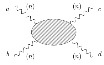
Figure 1: Elastic scattering of longitudinal modes of KK gauge bosons, $n+n\to n+n$, with the gauge index structure $a+b\to c+d$.

Figure 2: The four gauge diagrams contributing at tree level to the gauge boson elastic scattering amplitude.

3 How to bulid a realistic Higgsless model?

We have understood that it may be in principle possible to get a 5D theory without a Higgs that breaks electroweak symmetry, and is weakly coupled to a scale higher than the usual unitarity violation scale of the SM would be. However, this leaves us to show that one can actually build a model of this sort that gives the correct W/Z mass ratio, fermion couplings, fermion masses, etc. The first immediate question is regarding the masses of the gauge bosons and their KK modes. In a usual extra dimensional model the masses of the gauge fields are of the form

$$M_{n}\sim\frac{n}{R}$$ (6)

and is usually independent of the gauge couplings. This makes it hard to imagine that one could actually recover the usual tree-level SM relation

$$\frac{M_{W}^{2}}{M_{Z}^{2}}=\frac{g^{2}}{g^{2}+g^{\prime 2}},$$ (7)

and leaves us also to wonder how we could ever arrange to have the KK modes of the W and Z not appear at masses of around 2-3 times the ordinary gauge boson masses (which would have been excluded experimentally unless the couplings to the SM fermions are almost exactly vanishing).

The clue to finding a correct model can be obtained by understanding why (7) is obeyed in the first place in the SM. It is due to the global symmetry breaking pattern in the Higgs sector. The Higgs potential of the SM is invariant under the rotation of all four real components of the scalar, thus there is an approximate global $SO(4)\sim SU(2)_{L}\times SU(2)_{R}$ symmetry. When the Higgs gets a VEV this group is broken to $SU(2)_{D}$. Thus the aim is to build an extra dimensional theory where this is the actual symmetry breaking pattern, which will the automatically imply that the relation (7) has to be satisfied. One can guess [?] that there should be an $SU(2)_{L}\times SU(2)_{R}\times U(1)_{B-L}$ gauge group in the bulk of the extra dimension, but to really understand all the necessary parts [?] one needs to go to the AdS/CFT correspondence [?]. From this one learns that the bulk of an anti-de Sitter (AdS) space corresponds in “some sense” to a 4D conformal field theory (CFT). Moreover, if there are some gauge fields in the bulk of the AdS space this will imply that the CFT has a global symmetry, and the symmetries unbroken at the high scale (Planck brane) will remain as weakly gauged symmetries. While the symmetries that are broken on the Planck brane will be global symmetries of the CFT. Using these arguments as a guiding principle it is clear that one needs the following setup: there is an $SU(2)_{L}\times SU(2)_{R}\times U(1)_{B-L}$ gauge symmetry in the bulk of an AdS space [?], where the boundary conditions on the Planck brane break $SU(2)_{R}\times U(1)_{B-L}$ to $U(1)_{Y}$, while the boundary conditions on the TeV brane break $SU(2)_{L}\times SU(2)_{R}$ to $SU(2)_{D}$. This is illustrated in Fig. 3.

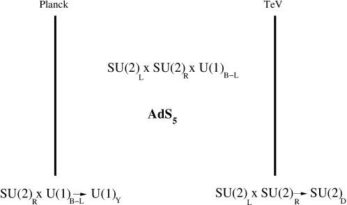
Figure 3: The symmetry breaking structure of the warped higgsless model.

Thus we will be considering a 5D gauge theory in the fixed gravitational background

$$ds^{2}=\left(\frac{R}{z}\right)^{2}\Big{(}\eta_{\mu\nu}dx^{\mu}dx^{\nu}-dz^{2}\Big{)}$$ (8)

where $z$ is on the interval $[R,R^{\prime}]$. We will not be considering gravitational fluctuations, that we are assuming that the Planck scale is sent to infinity, while the background is frozen to be the one given above. In RS-type models $R$ is typically $\sim 1/M_{Pl}$ and $R^{\prime}\sim{\rm TeV}^{-1}$. The BC’s corresponding to the symmetry breaking pattern discussed above is given by [?]:

$${\rm at}\ z=R^{\prime}: \left\{\begin{array}[]{l}\partial_{z}(A^{L\,a}_{\mu}+A^{R\,a}_{\mu})=0,\ A^{L\,a}_{\mu}-A^{R\,a}_{\mu}=0,\ \partial_{z}B_{\mu}=0,\\ (A^{L\,a}_{5}+A^{R\,a}_{5})=0,\ \partial_{z}(A^{L\,a}_{5}-A^{R\,a}_{5})=0,\ B_{5}=0.\end{array}\right.$$ (11)

$${\rm at}\ z=R: \left\{\begin{array}[]{l}\partial_{5}A^{L\,a}_{\mu}=0,\ A^{R\,1,2}_{\mu}=0,\\ \partial_{z}(g_{5}B_{\mu}+\tilde{g}_{5}A^{R\,3}_{\mu})=0,\ \tilde{g}_{5}B_{\mu}-g_{5}A^{R\,3}_{\mu}=0,\\ A^{L\,a}_{5}=0,\ A^{R\,a}_{5}=0,\ B_{5}=0.\end{array}\right.$$ (15)

These BC’s can be thought of as arising from Higgses on each brane in the limit of large VEVs which decouples the Higgs from gauge boson scattering [?]. The Higgs on the TeV brane is a bi-fundamental under the two $SU(2)$’s, while the Higgs on the Planck brane is a fundamental under $SU(2)_{R}$ and has charge $1/2$ under $U(1)_{B-L}$ so that a VEV in the lower component preserves $Y=T_{3}+B-L$.

The linearized Maxwell equation for the bulk gauge fields in the AdS background is given by

$$(\partial_{z}^{2}-\frac{1}{z}\partial_{z}+q^{2})\psi(z)=0,$$ (16)

where the solutions in the bulk are assumed to be of the form $A_{\mu}(q)e^{-iqx}\psi(z)$. The the KK mode expansion is given by the solutions to this equation which are of the form

$$\psi^{(A)}_{k}(z)=z\left(a^{(A)}_{k}J_{1}(q_{k}z)+b^{(A)}_{k}Y_{1}(q_{k}z)\right)~{},$$ (17)

where $A$ labels the corresponding gauge boson. Due to the mixing of the various gauge groups, the KK decomposition is slightly complicated but it is obtained by simply enforcing the BC’s:

$$B_{\mu}(x,z) = g_{5}\,a_{0}\gamma_{\mu}(x)+\sum_{k=1}^{\infty}\psi^{(B)}_{k}(z)\,Z^{(k)}_{\mu}(x)\,,$$ (18)

$$A^{L\,3}_{\mu}(x,z) = {\tilde{g}_{5}}\,a_{0}\gamma_{\mu}(x)+\sum_{k=1}^{\infty}\psi^{(L3)}_{k}(z)\,Z^{(k)}_{\mu}(x)\,,$$ (19)

$$A^{R\,3}_{\mu}(x,z) = {\tilde{g}_{5}}\,a_{0}\gamma_{\mu}(x)+\sum_{k=1}^{\infty}\psi^{(R3)}_{k}(z)\,Z^{(k)}_{\mu}(x)\,,$$ (20)

$$A^{L\,\pm}_{\mu}(x,z) = \sum_{k=1}^{\infty}\psi^{(L\pm)}_{k}(z)\,W^{(k)\,\pm}_{\mu}(x)\,,$$ (21)

$$A^{R\,\pm}_{\mu}(x,z) = \sum_{k=1}^{\infty}\psi^{(R\pm)}_{k}(z)\,W^{(k)\,\pm}_{\mu}(x)\,.$$ (22)

Here $\gamma(x)$ is the 4D photon, which has a flat wavefunction due to the unbroken $U(1)_{Q}$ symmetry, and $W^{(k)\,\pm}_{\mu}(x)$ and $Z^{(k)}_{\mu}(x)$ are the KK towers of the massive $W$ and $Z$ gauge bosons, the lowest of which are supposed to correspond to the observed $W$ and $Z$. To leading order in $1/R$ and for $\log\left(R^{\prime}/R\right)\gg 1$, the lightest solution for this equation for the mass of the $W^{\pm}$’s is

$$M_{W}^{2}=\frac{1}{R^{\prime 2}\log\left(\frac{R^{\prime}}{R}\right)}\,.$$ (23)

Note, that this result does not depend on the 5D gauge coupling, but only on the scales $R,R^{\prime}$. Taking $R=10^{-19}$ GeV^-1 will fix $R^{\prime}=2\cdot 10^{-3}$ GeV^-1. The lowest mass of the $Z$ tower is approximately given by

$$M_{Z}^{2}=\frac{g_{5}^{2}+2\tilde{g}_{5}^{2}}{g_{5}^{2}+\tilde{g}_{5}^{2}}\frac{1}{R^{\prime 2}\log\left(\frac{R^{\prime}}{R}\right)}\,.$$ (24)

If the SM fermions are localized on the Planck brane then the leading order expression for the 4D Weinberg angle will be given by

$$\sin\theta_{W}=\frac{\tilde{g}_{5}}{\sqrt{g_{5}^{2}+2\tilde{g}_{5}^{2}}}=\frac{g^{\prime}}{\sqrt{g^{2}+g^{\prime 2}}}.$$ (25)

Thus we can see that to leading order the SM expression for the W/Z mass ratio is reproduced in this theory as expected. In fact the full structure of the SM coupling is reproduced at the leading order in $1/\log R^{\prime}/R$, which implies that at the leading log level there is no $S$-parameter either. An $S$-parameter in this language would have manifested itself in an overall shift of the coupling of the Z compared to its SM value evaluated from the $W$ and $\gamma$ couplings, which are absent at this order of approximation. The corrections to the SM relations will appear in the next order of the log expansion, for which we will be showing the results later on. To evaluate the predictions of this model to a precision required by the measurements of the electroweak observables one needs to calculate at least the next order of corrections to the masses and couplings, together with the loop effects of the KK gauge bosons, and subtract the usual Higgs contributions.

4 Fermion masses

In the SM the Higgs serves a double purpose: it gives mass to the gauge bosons by breaking the electroweak symmetry, but it also provides a mass to the fermions via the Yukawa couplings. So our next task is to show that in the above presented warped higgsless model one can also reproduce the fermion masses via boundary conditions [?,?,?,?]. For this we need to first decide where we put the SM fermions in this theory. If we were to put them on the TeV brane then the fermions would only transform under $SU(2)_{D}\times U(1)_{B-L}$ which would imply that the spectrum is non-chiral. If the fermions were totally localized on the Planck brane then one would not be able to generate masses for them. So the only possible way is if the fermions are in the bulk, and thus feel both the Planck brane and the TeV brane. However, 5D fermions are Dirac fermions, thus for every 4D Weyl fermion one needs to introduce a Dirac fermion. The boundary conditions will then be chosen such that (as usually in a KK theory) the zero mode spectrum will be chiral. Next we summarize briefly the properties of 5D fermions in warped space. The action of a 5D fermion in warped space is generically given by

$$S=\int d^{5}x\sqrt{g}\left(\frac{i}{2}(\bar{\Psi}\,e_{a}^{M}\gamma^{a}D_{M}\Psi-D_{M}\bar{\Psi}\,e_{a}^{M}\gamma^{a}\Psi)-m\bar{\Psi}\Psi\right),$$ (26)

where $e_{a}^{M}$ is the generalization of the vierbein to higher dimensions (“fünfbein”) satisfying

$$e_{a}^{M}\eta^{ab}e^{N}_{b}=g^{MN},$$ (27)

the $\gamma^{a}$’s are the usual Dirac matrices, and $D_{M}$ is the covariant derivative including the spin connection term. For the AdS₅ metric in the conformal coordinates written above, $e_{M}^{a}=(R/z)\delta_{M}^{a}$, and $D_{\mu}\Psi=(\partial_{\mu}+\gamma_{\mu}\gamma_{5}/(4z))\Psi$, $D_{5}\Psi=\partial_{5}\Psi$, however the spin connection terms involved in the two covariant derivatives of (26) cancel each other and thus do not contribute in total to the action. Finally, in terms of two component spinors, the action is given by

$$S=\int d^{5}x\left(\frac{R}{z}\right)^{4}\left(-i\bar{\chi}\bar{\sigma}^{\mu}\partial_{\mu}\chi-i\psi\sigma^{\mu}\partial_{\mu}\bar{\psi}+\frac{1}{2}(\psi\overleftrightarrow{\partial_{5}}\chi-\bar{\chi}\overleftrightarrow{\partial_{5}}\bar{\psi})+\frac{c}{z}\left(\psi\chi+\bar{\chi}\bar{\psi}\right)\right),$$ (28)

where $c$ is the bulk Dirac mass in units of the AdS curvature $1/R$, and again $\overleftrightarrow{\partial_{5}}=\overrightarrow{\partial_{5}}-\overleftarrow{\partial_{5}}$ with the convention that the differential operators act only on the spinors and not on the metric factors. The localization properties of the zero modes are strongly dependent on the parameter $c$. For $c>1/2$ the left handed zero mode is localized near the Planck brane. Conversely, for $c<1/2$ the zero mode is thus localized near the TeV brane. In the AdS/CFT language [?] this corresponds to the fact that for $c>1/2$ the fermions will be elementary (since they are localized on the Planck brane), while for $c<1/2$ they are to be considered as composite bound states of the CFT modes (since they are peaked on the TeV brane). A right handed zero mode is localized on the Planck brane for $c<-1/2$, and on the TeV brane for $c>-1/2$.

We now discuss how to obtain the masses for the lepton sector of the warped higgsless model. The quark sector can be obtained similarly with slight modifications.

As always in a left–right symmetric model, the fermions are in the representations $(2,1,-1/2)$ and $(1,2,-1/2)$ of SU(2)${}_{L}\times$ SU(2)${}_{R}\times$ U(1)_B-L for left and right handed leptons respectively. Since we assume that the fermions live in the bulk, both of these are Dirac fermions, thus every chiral SM fermion is doubled (and the right handed neutrino is added similarly). Thus the left handed doublet can be written as

$$\left(\chi_{\nu_{L}},\bar{\psi}_{\nu_{L}},\chi_{e_{L}},\bar{\psi}_{e_{L}}\right)^{t}\,,$$ (29)

where $(\chi_{\nu_{L}},\chi_{e_{L}})$ will eventually correspond to the SM SU(2)_L doublet and $({\psi}_{\nu_{L}},{\psi}_{e_{L}})$ is its SU(2)_L antidoublet partner needed to form a complete 5D Dirac spinor. Similarly, the content of the right handed doublet is

$$\left(\chi_{\nu_{R}},\bar{\psi}_{\nu_{R}},\chi_{e_{R}},\bar{\psi}_{e_{R}}\right)^{t}\,,$$ (30)

where $(\psi_{\nu_{R}},\psi_{e_{R}})$ would correspond to the ’SM’ right-handed doublet, i.e., the right electron and the extra right neutrino, while $(\chi_{\nu_{R}},\chi_{e_{R}})$ is its antidoublet partner again needed to form a complete 5D Dirac spinor. Without boundary terms the BC’s would be just $\chi_{R}=\psi_{L}=0$ on both branes. This will ensure that the zero modes will be given by $\chi_{L}$ and $\psi_{R}$. In order to make the zero modes acquire small masses, one can add a Dirac mass on the TeV brane. This is because on the TeV brane the theory is non-chiral. This will modify the BC’s on the TeV brane to

$${\psi_{L}}_{|R^{\prime\,-}}=-M_{D}R^{\prime}\,{\psi_{R}}_{|R^{\prime\,-}}$$ (31)

$${\chi_{R}}_{|R^{\prime\,-}}=M_{D}R^{\prime}\,{\chi_{L}}_{|R^{\prime\,-}}$$ (32)

On the Planck brane the unbroken gauge group is $SU(2)_{L}\times U(1)_{Y}$ so we can add a Majorana mass to the right handed neutrino on the Planck brane. This will lead to a BC of the form

$$\psi_{\nu_{R}}=MR\,\chi_{\nu_{R}}.$$ (33)

Together with the bulk equations of motion these BC’s lead to the following approximate mass spectrum for the neutrinos

$$m_{0}\sim\frac{fM_{D}^{2}}{M^{2}},$$ (34)

which is of the typical see-saw type since the Dirac mass, $M_{D}$, which is of the same order as that of the electron mass, is suppressed by the large masses of the right handed neutrinos localized on the brane. Similarly one can show that a realistic spectrum is achievable in this simple toy model for the charged leptons is also achievable.

5 Electroweak precision observables

Next we will discuss the leading corrections to the electroweak precision observables in the warped higgsless model [?,?,?,?,?]. In the following we will use the oblique corrections $S$, $T$ and $U$ to fit the $Z$-pole observables, mainly measured at LEP1. These three parameters are sufficient for predicting all of those observables. In [?], Barbieri et al. proposed a new enlarged set of parameters to also take into account the differential cross section measurements at LEP2. The only additional information contained in these parameters is the bound on the coefficients of the four-Fermi operators that are generated by the exchange of gauge boson KK modes.In our approach we simply use the bounds on $S,T$ and $U$ from the $Z$-pole observables, while the bounds on the four Fermi operators are taken into account by directly imposing the constraints on new gauge bosons from LEP2 and from the direct searches at Tevatron.

Perturbatively the $S$ parameter “counts” the number of degrees of freedom that participate in the electroweak sector, while the $T$ parameter measures the amount of additional isospin breaking. Contributions to $U$ are typically very small. Both $S$ and $T$ must be typically small ($<0.25$) in order to be compatible with precision electroweak measurements.

Electroweak symmetry breaking sectors that are more complicated than a 4D Higgs doublet tend to have positive $S$ parameters of order 1. In Higgsless models with a warped extra dimension it has been shown [?] that both the ratio of $SU(2)_{L}$ and $SU(2)_{R}$ couplings, $g_{5R}/g_{5L}$ as well as kinetic terms on the TeV brane affect the $S$ and $T$ parameters in important ways. With no brane kinetic terms and $g_{5R}=g_{5L}$, $S=1.15$ and $T=0$. Increasing the ratio $g_{5R}/g_{5L}$ reduces $S$ to

$$S\approx\frac{6\pi}{g^{2}\log\frac{R^{\prime}}{R}}\frac{2}{1+\frac{g_{5R}^{2}}{g_{5L}^{2}}}$$ (35)

while keeping $T\approx 0$. A qualitatively similar effect is induced by Planck brane kinetic terms whose dimensionless coefficient we denote by $r$, the only difference being in the couplings of the gauge bosons, thus affecting the bounds on direct $Z^{\prime}$ searches. It was shown in [?] that the TeV brane kinetic terms produce further corrections. We denote the dimensionless coefficient of the $SU(2)_{D}$ kinetic term on the TeV brane $\tau$ and for the $U(1)_{B-L}$ by $\tau^{\prime}$. The non-Abelian brane kinetic term gives a correction to $S$ at first order, multiplying the previous result by $1+\frac{4}{3}\frac{\tau}{R}$, while giving a very small positive contribution to $T$. The $\tau^{\prime}$ corrections are more complicated, and more interesting. The first effects appear at quadratic order, and they give negative corrections to both $S$ and $T$. The Abelian brane kinetic term, $\tau^{\prime}$, also has the effect of reducing the mass of the lightest neutral KK gauge boson resonance. We scanned the model in this 3D parameter space, $(g_{5R}/g_{5L},\tau,\tau^{\prime})$, to uncover regions allowed by experiments. In Fig.4 we show combined plots for four values of $g_{5R}/g_{5L}$= 1, 2, 2.5, 3. In order to satisfy both precision tests and LEP2/Tevatron bounds, a large $g_{5R}/g_{5L}$ ratio is required. In this case, however, the masses of the resonances are raised, making them possibly ineffective in restoring partial wave unitarity and leading to strong coupling below $2$ TeV. These results are in agreement with the conclusions of refs. [?,?].

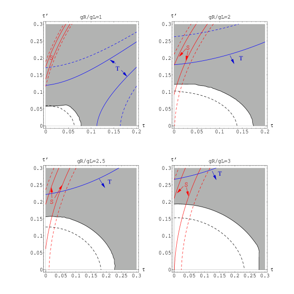
Figure 4: Combined plots of the experimental constraints on Higgsless models for different values of the $g_{5R}/g_{5L}$ ratio, in the parameter space $\tau$–$\tau^{\prime}$ (normalized by $R\log R^{\prime}/R$). The solid contours for $S$ (red) and $T$ (blue) are at $0.25$; the dashed contours at $0.5$. The black solid (dashed) line corresponds to a deviation in the differential cross section of $3\%$ ($2\%$) at LEP2. The shaded region is excluded by a deviation larger that $3\%$ at LEP and/or direct search at Run1 at Tevatron.

In the following, we would like to focus on an alternative solution [?] to the $S$ problem which has additional beneficial side-effects. It has been known for a long time in Randall-Sundrum (RS) models with a Higgs that the effective $S$ parameter is large and negative [?] if the fermions are localized on the TeV brane as originally proposed. When the fermions are localized on the Planck brane the contribution to $S$ is positive, and so for some intermediate localization the $S$ parameter vanishes, as first pointed out for RS models by Agashe et al.[?]. The reason for this is fairly simple. Since the $W$ and $Z$ wavefunctions are approximately flat, and the gauge KK mode wavefunctions are orthogonal to them, when the fermion wavefunctions are also approximately flat the overlap of a gauge KK mode with two fermions will approximately vanish. Since it is the coupling of the gauge KK modes to the fermions that induces a shift in the $S$ parameter, for approximately flat fermion wavefunctions the $S$ parameter must be small. Note that not only does reducing the coupling to gauge KK modes reduce the $S$ parameter, it also weakens the experimental constraints on the existence of light KK modes. This case of delocalized bulk fermions is not covered by the no–go theorem of [?], since there it was assumed that the fermions are localized on the Planck brane.

In order to quantify these statements, it is sufficient to consider a toy model where all the three families of fermions are massless and have a universal delocalized profile in the bulk. Before showing some numerical results, it is useful to understand the analytical behavior of $S$ in interesting limits. For fermions almost localized on the Planck brane, it is possible to expand the result for the $S$-parameter in powers of $(R/R^{\prime})^{2c_{L}-1}\ll 1$. The leading terms, also expanding in powers of $1/\log$, are:

$$S=\frac{6\pi}{g^{2}\,\log\frac{R^{\prime}}{R}}\left(1-\frac{4}{3}\frac{2c_{L}-1}{3-2c_{L}}\left(\frac{R}{R^{\prime}}\right)^{2c_{L}-1}\log\frac{R^{\prime}}{R}\right)~{},$$ (36)

and $U\approx T\approx 0$. The above formula is actually valid for $1/2<c_{L}<3/2$. For $c_{L}>3/2$ the corrections are of order $(R^{\prime}/R)^{2}$ and numerically negligible. As we can see, as soon as the fermion wave function starts leaking into the bulk, $S$ decreases.

Another interesting limit is when the profile is almost flat, $c_{L}\approx 1/2$. In this case, the leading contributions to $S$ are:

$$S=\frac{2\pi}{g^{2}\,\log\frac{R^{\prime}}{R}}\left(1+(2c_{L}-1)\,\log\frac{R^{\prime}}{R}+\mathcal{O}\left((2c_{L}-1)^{2}\right)\right)~{}.$$ (37)

In the flat limit $c_{L}=1/2$, $S$ is already suppressed by a factor of 3 with respect to the Planck brane localization case. Moreover, the leading terms cancel out for:

$$c_{L}=\frac{1}{2}-\frac{1}{2\,\log\frac{R^{\prime}}{R}}\approx 0.487~{}.$$ (38)

For $c_{L}<1/2$, $S$ becomes large and negative and, in the limit of TeV brane localized fermions ($c_{L}\ll 1/2$):

$$S=-\frac{16\pi}{g^{2}}\frac{1-2c_{L}}{5-2c_{L}}~{},$$ (39)

while, in the limit $c_{L}\rightarrow-\infty$:

$$T \rightarrow \frac{2\pi}{g^{2}\,\log\frac{R^{\prime}}{R}}(1+\tan^{2}\theta_{W})\approx 0.5~{},$$ (40)

$$U \rightarrow -\frac{8\pi}{g^{2}\,\log\frac{R^{\prime}}{R}}\frac{\tan^{2}\theta_{W}}{2+\tan^{2}\theta_{W}}\frac{1}{c_{L}}\approx 0~{}.$$ (41)

Figure 5: Plots of the oblique parameters as function of the bulk mass of the reference fermion. The values on the right correspond to localization on the Planck brane. $S$ vanishes for $c=0.487$.

In Fig. 5 we show the numerical results for the oblique parameters as function of $c_{L}$. We can see that, after vanishing for $c_{L}\approx 1/2$, $S$ becomes negative and large, while $T$ and $U$ remain smaller. With $R$ chosen to be the inverse Planck scale, the first KK resonance appears around $1.2$ TeV, but for larger values of $R$ this scale can be safely reduced down below a TeV. As already discussed in the previous section, such resonances will be weakly coupled to almost flat fermions and can easily avoid the strong bounds from direct searches at LEP or Tevatron. If we are imagining that the AdS space is a dual description of an approximate conformal field theory (CFT), then $1/R$ is the scale where the CFT is no longer approximately conformal and perhaps becomes asymptotically free. Thus it is quite reasonable that the scale $1/R$ would be much smaller than the Planck scale.

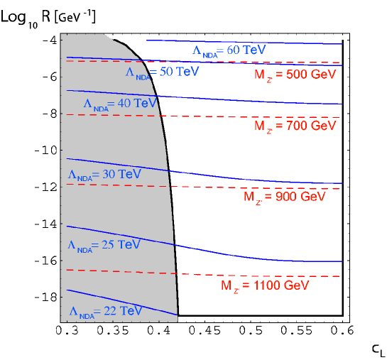
Figure 6: Contour plots of $\Lambda_{\rm NDA}$ (solid blue lines) and $M_{Z^{(1)}}$ (dashed red lines) in the parameter space $c_{L}$–$R$. The shaded region is excluded by direct searches of light $Z^{\prime}$ at LEP.

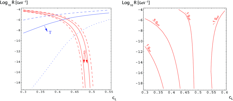
Figure 7: On the left, contours of $S$ (red), for $|S|=0.25$ (solid) and $0.5$ (dashed) and $T$ (blue), for $|T|=0.1$ (dotted), $0.3$ (solid) and $0.5$ (dashed), as function of $c_{L}$ and $R$. On the right, contours for the generic suppression of fermion couplings to the first resonance with respect to the SM value. In particular we plotted the couplings of a lh down–type massless quark with the $Z^{\prime}$. The region for $c_{L}$, allowed by $S$, is between $0.43\div 0.5$, where the couplings are suppressed at least by a factor of 10.

In Fig. 6 we have plotted the value of the NDA scale (4) as well as the mass of the first resonance in the $(c_{L}-R)$ plane. Increasing $R$ also affects the oblique corrections. However, while it is always possible to reduce $S$ by delocalizing the fermions, $T$ increases and puts a limit on how far $R$ can be raised. One can also see form Fig. 7 that in the region where $|S|<0.25$, the coupling of the first resonance with the light fermions is generically suppressed to less than $10\%$ of the SM value. This means that the LEP bound of $2$ TeV for SM–like $Z^{\prime}$ is also decreased by a factor of 10 at least (the correction to the differential cross section is roughly proportional to $g^{2}/M_{Z^{\prime}}^{2}$). In the end, values of $R$ as large as $10^{-7}$ GeV^-1 are allowed, where the resonance masses are around $600$ GeV. So, even if, following the analysis of [?], we take into account a factor of roughly $1/4$ in the NDA scale, we see that the appearance of strong coupling regime can be delayed up to $10$ TeV. At the LHC it will be very difficult to probe $WW$ scattering above 3 TeV.

6 Flavor issues

Finally we will address some issues about flavor physics arising in this scenario. First we will consider the eventual presence of flavor changing neutral currents (FCNC) induced either by higher dimension operators or by non–universal corrections. Next, we will briefly discuss the problems surrounding the inclusion of the third family of quarks in the picture.

A generic 4-fermi operator would be given by the following expression in this model:

$$\int d^{4}x\ \frac{1}{\Lambda_{FCNC}^{2}}\ \bar{\chi}_{u_{L}}\gamma^{\mu}\chi_{u_{L}}\ \bar{\chi}_{d_{L}}\gamma_{\mu}\chi_{d_{L}}.$$ (42)

After putting in the wave functions of the zero modes one can estimate the scale of suppression of the flavor changing operators as a function of the $c$’s:

$$\Lambda_{FCNC}^{2}\approx\frac{(R/R^{\prime})^{2-4c_{L}}\log(R^{\prime}/R)}{R^{\prime 2}}.$$ (43)

For $1/R^{\prime}\sim 1$ TeV, to get a suppression factor of $10^{3}$ TeV, $c_{L}$ would have to be bigger than $0.57$. Clearly the values of $c_{L}$ used to reduce the $S$ parameter do not fulfill this criterion, which means that the set-up fails to naturally explain the absence of FCNC and additional flavor symmetries in 5D would be necessary. It is however relatively easy to impose such a flavor symmetry in the bulk and on the TeV brane and naturally break it close to the Planck brane. Due to the small overlap of the fermion wavefunctions on the Planck brane, the suppression scale of the four-Fermi operators will be significantly increased.

The major challenge facing Higgsless models is the incorporation of the third family of quarks. There is a tension [?,?] in obtaining a large top quark mass without deviating from the observed bottom couplings with the $Z$. It can be seen in the following way. The top quark mass is proportional both to the Dirac mixing $M_{D}$ on the TeV brane and the overall scale of the extra dimension set by $1/R^{\prime}$. For $c_{L}\sim 0.5$ (or larger) it is in fact impossible to obtain a heavy enough top quark mass (at least for $g_{5R}=g_{5L}$). The reason is that for $M_{D}R^{\prime}\gg 1$ the light mode mass saturates at

$$m_{top}^{2}\sim\frac{2}{R^{\prime 2}\log\frac{R^{\prime}}{R}}\,,$$ (44)

which gives for this case $m_{top}\leq\sqrt{2}M_{W}$. Thus one needs to localize the top and the bottom quarks closer to the TeV brane. However, even in this case a sizable Dirac mass term on the TeV brane is needed to obtain a heavy enough top quark. The consequence of this mass term is the boundary condition for the bottom quarks

$$\chi_{bR}=M_{D}R^{\prime}\,\chi_{bL}.$$ (45)

This implies that if $M_{D}R^{\prime}\sim 1$ then the left handed bottom quark has a sizable component also living in an $SU(2)_{R}$ multiplet, which however has a coupling to the $Z$ that is different from the SM value. Thus there will be a large deviation in the $Zb_{L}\bar{b}_{L}$. Note, that the same deviation will not appear in the $Zb_{R}\bar{b}_{R}$ coupling, since the extra kinetic term introduced on the Planck brane to split top and bottom will imply that the right handed $b$ lives mostly in the induced fermion on the Planck brane which has the correct coupling to the $Z$.

The only way of getting around this problem would be to raise the value of $1/R^{\prime}$, and thus lower the necessary mixing on the TeV brane needed to obtain a heavy top quark. One way of raising the value of $1/R^{\prime}$ is by increasing the ratio $g_{5R}/g_{5L}$ (at the price of making also the gauge KK modes heavier and thus the theory more strongly coupled).

Another generic problem arising from the large value of the top-quark mass in models with warped extra dimensions comes from the isospin violations in the KK sector of the top and the bottom quarks. If the spectrum of the top and bottom KK modes is not sufficiently degenerate, the loop corrections involving these KK modes to the $T$-parameter could be large. This possibility was first pointed out in [?,?].

7 Conclusions

We have discussed the possibility of breaking the electroweak symmetry by boundary conditions rather than with a scalar Higgs. We have found that this may indeed be possible in theories with extra dimensions, and that in this case the scale of unitarity violation due to the absence of the Higgs scalar could be significantly delayed due to the exchange of the massive KK modes of the gauge bosons. In order to find a realistic model the presence of the custodial $SU(2)$ symmetry has to be guaranteed, which leads us naturally to the warped higgsless model. In this model the W/Z mass ratio is automatically the correct one, and there is a simple way to introduce a splitting between the lightest KK modes (to be identified with the ordinary W and Z) and the next ones. We have shown that fermions can be similarly incorporated into this picture. In the simplest model the prediction for the electroweak $S$-parameter comes out to be too large, however one can modify the structure of the light fermions to be able to suppress the $S$-parameter. The main unresolved issue is the incorporation of a sufficiently heavy top quark without inducing a large shift in the $Zb\bar{b}$ coupling.

8 Acknowledgements

I thank Giacomo Cacciapaglia, Christophe Grojean, Jay Hubisz, Hitoshi Murayama, Luigi Pilo, Yuri Shirman and John Terning for collaborations on [?,?,?,?,?] which were summarized in this talk. I thank the organizers of the SUSY 2004 conference in Tsukuba, Japan for inviting me and for providing a stimulating athmosphere. This research is supported in part by the DOE OJI grant DE-FG02-01ER41206 and in part by the NSF grants PHY-0139738 and PHY-0098631.

References

- [1] C. Csáki, C. Grojean, H. Murayama, L. Pilo and J. Terning, Phys. Rev. D 69, 055006 (2004) [arXiv:hep-ph/0305237].
- [2] C. Csáki, C. Grojean, L. Pilo and J. Terning, Phys. Rev. Lett. 92, 101802 (2004) [arXiv:hep-ph/0308038].
- [3] Y. Nomura, JHEP 0311, 050 (2003) [arXiv:hep-ph/0309189].
- [4] R. Barbieri, A. Pomarol and R. Rattazzi, Phys. Lett. B 591, 141 (2004) [arXiv:hep-ph/0310285].
- [5] C. Csáki, C. Grojean, J. Hubisz, Y. Shirman and J. Terning, Phys. Rev. D 70, 015012 (2004) [arXiv:hep-ph/0310355].
- [6] H. Davoudiasl, J. L. Hewett, B. Lillie and T. G. Rizzo, Phys. Rev. D 70, 015006 (2004) [arXiv:hep-ph/0312193].
- [7] G. Burdman and Y. Nomura, Phys. Rev. D 69, 115013 (2004) [arXiv:hep-ph/0312247].
- [8] G. Cacciapaglia, C. Csáki, C. Grojean and J. Terning, Phys. Rev. D 70, 075014 (2004) [arXiv:hep-ph/0401160].
- [9] H. Davoudiasl, J. L. Hewett, B. Lillie and T. G. Rizzo, JHEP 0405, 015 (2004) [arXiv:hep-ph/0403300]; J. L. Hewett, B. Lillie and T. G. Rizzo, JHEP 0410, 014 (2004) [arXiv:hep-ph/0407059].
- [10] R. Barbieri, A. Pomarol, R. Rattazzi and A. Strumia, Nucl. Phys. B 703, 127 (2004) [arXiv:hep-ph/0405040].
- [11] R. Foadi, S. Gopalakrishna and C. Schmidt, JHEP 0403, 042 (2004) [arXiv:hep-ph/0312324]; R. Casalbuoni, S. De Curtis and D. Dominici, Phys. Rev. D 70, 055010 (2004) [arXiv:hep-ph/0405188].
- [12] G. Cacciapaglia, C. Csaki, C. Grojean and J. Terning, arXiv:hep-ph/0409126.
- [13] R. Foadi, S. Gopalakrishna and C. Schmidt, arXiv:hep-ph/0409266.
- [14] R. S. Chivukula, E. H. Simmons, H. J. He, M. Kurachi and M. Tanabashi, Phys. Rev. D 70, 075008 (2004) [arXiv:hep-ph/0406077]. R. S. Chivukula, H. J. He, M. Kurachi, E. H. Simmons and M. Tanabashi, Phys. Lett. B 603, 210 (2004) [arXiv:hep-ph/0408262].
- [15] H. Georgi, [arXiv:hep-ph/0408067].
- [16] M. Perelstein, JHEP 0410, 010 (2004) [arXiv:hep-ph/0408072].
- [17] T. Ohl and C. Schwinn, Phys. Rev. D 70, 045019 (2004) [arXiv:hep-ph/0312263]. C. Schwinn, Phys. Rev. D 69, 116005 (2004) [arXiv:hep-ph/0402118].
- [18] J. Hirn and J. Stern, Eur. Phys. J. C 34, 447 (2004) [arXiv:hep-ph/0401032].
- [19] N. Evans and P. Membry, arXiv:hep-ph/0406285.
- [20] S. Gabriel, S. Nandi and G. Seidl, Phys. Lett. B 603, 74 (2004) [arXiv:hep-ph/0406020]. T. Nagasawa and M. Sakamoto, Prog. Theor. Phys. 112, 629 (2004) [arXiv:hep-ph/0406024]. C. D. Carone and J. M. Conroy, Phys. Rev. D 70, 075013 (2004) [arXiv:hep-ph/0407116].
- [21] M. Papucci, [arXiv:hep-ph/0408058].
- [22] Y. Nomura, Talk at SUSY 2004, this volume.
- [23] H. Davoudiasl, Talk at SUSY 2004, this volume.
- [24] G. Cacciapaglia, Talk at SUSY 2004, this volume, arXiv:hep-ph/0409158.
- [25] G. Seidel, Talk at SUSY 2004, this volume, arXiv:hep-ph/0409162.
- [26] M. Kurachi, Talk at SUSY 2004, this volume, arXiv:hep-ph/0409134.
- [27] R. S. Chivukula, D. A. Dicus and H. J. He, Phys. Lett. B 525, 175 (2002) [arXiv:hep-ph/0111016]; R. S. Chivukula, D. A. Dicus, H. J. He and S. Nandi, Phys. Lett. B 562, 109 (2003) [arXiv:hep-ph/0302263]. R. S. Chivukula and H. J. He, Phys. Lett. B 532, 121 (2002) [arXiv:hep-ph/0201164]; S. De Curtis, D. Dominici and J. R. Pelaez, Phys. Lett. B 554, 164 (2003) [arXiv:hep-ph/0211353]; and Phys. Rev. D 67, 076010 (2003) [arXiv:hep-ph/0301059]; Y. Abe, N. Haba, Y. Higashide, K. Kobayashi and M. Matsunaga, Prog. Theor. Phys. 109, 831 (2003) [arXiv:hep-th/0302115].
- [28] K. Agashe, A. Delgado, M. J. May and R. Sundrum, JHEP 0308, 050 (2003) [arXiv:hep-ph/0308036].
- [29] N. Arkani-Hamed, M. Porrati and L. Randall, JHEP 0108, 017 (2001) [arXiv:hep-th/0012148]; R. Rattazzi and A. Zaffaroni, JHEP 0104, 021 (2001) [arXiv:hep-th/0012248];
- [30] C. Csáki, J. Erlich and J. Terning, Phys. Rev. D 66, 064021 (2002) [arXiv:hep-ph/0203034].
- [31] K. Agashe, R. Contino and A. Pomarol, arXiv:hep-ph/0412089.