Probing Generalized Parton Distributions with Neutrino Beams

Abstract

A short review of form factors, parton distribution functions and generalized parton distributions is given. A possible application of generalized parton distributions in the weak sector is discussed.

PACS number(s): 13.15.+g, 13.40.-f, 13.40.Gp, 13.60.-r, 13.60.Fz, 13.60.Hb

I Introduction

Specific aspects of hadronic structure are described by several different phenomenological functions. Form factors, usual parton distribution functions (PDFs) and distribution amplitudes are the so-called “old” phenomenological functions since they have been around for a long time. On the other hand, the concept of generalized parton distributions (GPDs) Muller:1998fv ; Ji:1996ek ; Ji:1996nm ; Radyushkin:1996nd ; Radyushkin:1997ki (for recent reviews, see Goeke:2001tz ; Diehl:2003ny ) is new. These “new” phenomenological functions are hybrids of the “old” ones, and therefore they provide a unified and more detailed description of the hadronic structure.

In recent years, significant effort was made to access GPDs through the measurement of hard exclusive electro-production processes. The simplest process in this respect is the deeply virtual Compton scattering (DVCS) process, i.e. an electron scatters off a nucleon producing a photon in the final state. Using the neutrino beam instead we extend the DVCS process into the weak sector, where one expects to be sensitive to a different flavor decomposition of GPDs, and further, due to the presence of the axial part of the V-A interaction also sensitive to a different set of GPDs. In addition, the weak DVCS process allows us to study flavor non-diagonal GPDs, e.g. in the neutron-to-proton transition.

Detailed study of weak deeply virtual Compton scattering with electron and neutrino beams will be presented in a forthcoming paper.

II Phenomenological Functions

Among phenomenological functions we discuss form factors, usual parton distribution functions and generalized parton distributions.

II.1 Form Factors

Form factors are defined through matrix elements of electromagnetic and weak currents between the hadronic states. In particular, the matrix element of the vector current between the nucleon states $N\left(p_{1},s_{1}\right)$ and $N\left(p_{2},s_{2}\right)$ is parametrized in terms of the nucleon electromagnetic form factors, i.e. Dirac and Pauli form factors,

$$\left\langle N\left(p_{2},s_{2}\right)\right|J_{V}^{\mu}\left(0\right)\left|N\left(p_{1},s_{1}\right)\right\rangle = \overline{u}\left(p_{2},s_{2}\right)\left[\gamma^{\mu}F_{1}\left(t\right)-i\sigma^{\mu\nu}\frac{r_{\nu}}{2M}F_{2}\left(t\right)\right]u\left(p_{1},s_{1}\right),$$ (1)

where $r=p_{1}-p_{2}$ is the overall momentum transfer, the invariant $t=r^{2}$ and M denotes the nucleon mass. In the case of the axial vector current one has the axial and pseudoscalar form factors,

$$\left\langle N\left(p_{2},s_{2}\right)\right|J_{A}^{\mu}\left(0\right)\left|N\left(p_{1},s_{1}\right)\right\rangle = \overline{u}\left(p_{2},s_{2}\right)\left[\gamma^{\mu}\gamma_{5}g_{A}\left(t\right)-\gamma_{5}\frac{r^{\mu}}{2M}g_{P}\left(t\right)\right]u\left(p_{1},s_{1}\right).$$ (2)

Both currents in Eqs. (1) and (2) are given by the sum of their flavor components, $J_{V}^{\mu}\left(0\right)=\sum_{f}Q_{f}\bar{\psi}_{f}\left(0\right)\gamma^{\mu}\psi_{f}\left(0\right)$ and $J_{A}^{\mu}\left(0\right)=\sum_{f}Q_{Af}\bar{\psi}_{f}\left(0\right)\gamma^{\mu}\gamma_{5}\psi_{f}\left(0\right)$, where $Q_{f}$ and $Q_{Af}$ are the electric (in units of $\left|e\right|$) and axial charges of the quark of flavor f, respectively. A similar decomposition holds for the form factors, $F_{1,2}\left(t\right)=\sum_{f}Q_{f}F_{1,2f}\left(t\right)$ and $g_{A,P}\left(t\right)=\sum_{f}Q_{Af}g_{A,Pf}\left(t\right)$. Their limiting values at $t=0$ are known, e.g. Dirac and Pauli form factors give the total electric charge of the nucleon and its anomalous magnetic moment.

In particular, the nucleon electromagnetic form factors can be measured through elastic electron-nucleon scattering,

$$e^{-}N \longrightarrow e^{-}N.$$ (3)

The process is shown in one photon-exchange approximation in Figure 1, left.

II.2 Usual Parton Distribution Functions

PDFs are defined through forward matrix elements of quark/gluon fields separated by light-like distances. For the unpolarized case one has

$$\left\langle N\left(p_{1},s_{1}\right)\right|\bar{\psi}_{f}\left(-z/2\right)\gamma^{\mu}\psi_{f}\left(z/2\right)\left|N\left(p_{1},s_{1}\right)\right\rangle_{z^{2}=0} = \overline{u}\left(p_{1},s_{1}\right)\gamma^{\mu}u\left(p_{1},s_{1}\right)$$ (4)

$$\times\int_{0}^{1}dx\;\left[e^{-ix\left(p_{1}z\right)}q_{f}\left(x\right)-e^{ix\left(p_{1}z\right)}\overline{q}_{f}\left(x\right)\right],$$

and for the polarized one

$$\left\langle N\left(p_{1},s_{1}\right)\right|\bar{\psi}_{f}\left(-z/2\right)\gamma^{\mu}\gamma_{5}\psi_{f}\left(z/2\right)\left|N\left(p_{1},s_{1}\right)\right\rangle_{z^{2}=0} = \overline{u}\left(p_{1},s_{1}\right)\gamma^{\mu}\gamma_{5}u\left(p_{1},s_{1}\right)$$ (5)

$$\times\int_{0}^{1}dx\;\left[e^{-ix\left(p_{1}z\right)}\Delta q_{f}\left(x\right)+e^{ix\left(p_{1}z\right)}\Delta\overline{q}_{f}\left(x\right)\right].$$

To make connection with GPDs, which are usually discussed in the region $-1\leq x\leq 1$, it is convenient to introduce new distribution functions,

$$\widetilde{q}_{f}\left(x\right)=\left\{\begin{array}[]{cc}q_{f}\left(x\right)&x>0\\ -\overline{q}_{f}\left(-x\right)&x<0\\ \end{array}\right.$$ (6)

and

$$\Delta\widetilde{q}_{f}\left(x\right)=\left\{\begin{array}[]{cc}\Delta q_{f}\left(x\right)&x>0\\ \Delta\overline{q}_{f}\left(-x\right)&x<0\\ \end{array}\right.$$ (7)

and alternatively, write the integrals over x in Eqs. (4) and (5) as

$$\int_{0}^{1}dx\;\left[e^{-ix\left(p_{1}z\right)}q_{f}\left(x\right)-e^{ix\left(p_{1}z\right)}\overline{q}_{f}\left(x\right)\right] = \int_{-1}^{1}dx\;e^{-ix\left(p_{1}z\right)}\widetilde{q}_{f}\left(x\right),$$

$$\int_{0}^{1}dx\;\left[e^{-ix\left(p_{1}z\right)}\Delta q_{f}\left(x\right)+e^{ix\left(p_{1}z\right)}\Delta\overline{q}_{f}\left(x\right)\right] = \int_{-1}^{1}dx\;e^{-ix\left(p_{1}z\right)}\Delta\widetilde{q}_{f}\left(x\right).$$ (8)

Furthermore, one observes that the definition of PDFs has the form of the plane wave decomposition. Thus it allows us to give the momentum space interpretation: $q_{f}\left(x\right)/\overline{q}_{f}\left(x\right)$ is the probability to find the quark/antiquark of flavor f carrying the momentum $xp_{1}$ inside a fast-moving nucleon having the momentum $p_{1}$.

PDFs have been intensively studied in hard inclusive processes for the last three decades. The classic example in this respect is the deeply inelastic scattering (DIS) process, i.e. inclusive scattering of high energy leptons on the nucleon,

$$e^{-}N \longrightarrow e^{-}X,$$ (9)

shown in Figure 1, right. It played a key role in revealing the quark structure of the nucleon. The structure functions, accessed in the DIS process, are directly expressed in terms of PDFs. Through the optical theorem, its cross section is given by the imaginary part of the forward virtual Compton scattering amplitude (see Figure 2). The summation over X reflects the inclusive nature of the nucleon structure description by PDFs.

In the Bjorken regime, where the space-like momentum transfer is sufficiently large together with large total center-of-mass energy of the photon-nucleon system, $-q_{1}^{2}$ and $\left(p_{1}+q_{1}\right)^{2}\rightarrow\infty$, while the ratio $x_{B}\equiv-q_{1}^{2}/2\left(p_{1}\cdot q_{1}\right)$ is finite, perturbative QCD factorization works. In other words, the forward virtual Compton scattering amplitude factorizes into perturbatively calculable hard scattering process at the level of quarks and gluons, and process independent matrix elements which contain the soft non-perturbative information about the nucleon structure represented by the blob (see Figure 3). We recall that these forward matrix elements consist of quark and gluon operators, whose fields are separated by a light-like distance. They are described and parametrized in terms of PDFs. Schematically, QCD factorization allows us to write the amplitude in the form of the so-called handbag diagrams. Moreover, the leading contribution in the lowest order in the strong coupling constant $\alpha_{s}$ is given by two (s- and u-channel) handbag diagrams in which the hard propagator is convoluted with the PDFs. Taking the imaginary part of the forward virtual Compton scattering amplitude generates the delta function, $\Im\left[\left(xp_{1}\pm q_{1}\right)^{2}+i\epsilon\right]^{-1}\approx\delta\left(x\mp x_{B}\right)/2\left(p_{1}\cdot q_{1}\right)$. Hence in the DIS process one measures the PDF $\widetilde{q}_{f}\left(x\right)$ at two points, $x=\pm x_{B}$, with $x=x_{B}$ corresponding to the quark PDF and $x=-x_{B}$ for that of antiquarks.

II.3 Generalized Parton Distributions

A more recent attempt to use perturbative QCD to extract new information about the hadronic structure is the study of hard exclusive electro-production processes, in particular the DVCS process. This is a much more difficult task due to the small cross sections. However, high energy and high luminosity electron accelerators combined with large acceptance spectrometers give a unique opportunity to perform precision studies of such reactions. The DVCS process can be accessed through the reaction

$$e^{-}N \longrightarrow e^{-}N\gamma.$$ (10)

It turns out that factorization into short and long distance dynamics is more general. Having large space-like virtuality of the initial photon while the final state photon is on shell is sufficient for QCD factorization to work. In contrast to the DIS process, the outgoing photon is real, and henceforth, the overall momentum transfer is not equal to zero. In the leading handbag approximation, the so-called non-forward virtual Compton scattering amplitude is dominated by two diagrams (see Figure 4). The lower blob now contains the non-forward matrix elements of the same quark and gluon operators as in the forward case. They are parametrized in terms of GPDs.

It is convenient to introduce the average of the nucleon momenta, $p=\left(p_{1}+p_{2}\right)/2$, and treat the initial and final hadron in a symmetric way (see Figure 5). In this scheme, at the leading twist-2 level, the nucleon structure information can be parametrized in terms of two unpolarized and two polarized GPDs denoted by $H,\;E\;\mathrm{and}\;\widetilde{H},\;\widetilde{E}$, respectively. They are functions of three variables $\left(x,\xi,t\right)$, and further they are defined for each quark flavor f. In addition to the usual light-cone momentum fraction x, GPDs also depend upon another scaling variable, the skewness parameter $\xi=r_{\|}/2p_{\|}$, specifying the longitudinal momentum asymmetry, and upon the invariant t. The variables x and $\xi$ solely characterize the longitudinal momenta of the partons involved, however, the t-dependence of GPDs is related to their transverse momenta. Thus one can simultaneously access the longitudinal momentum and transverse position of the parton in the infinite momentum frame Burkardt:2000za . Furthermore, by removing the quark with the light-cone momentum fraction $x+\xi$ and replacing it with the quark of the momentum fraction $x-\xi$, one can say that GPDs measure the coherence between two different quark momentum states of the nucleon, i.e. the quark momentum correlations in the nucleon, whereas usual PDFs yield only the probability that a quark carries a fraction x of the nucleon momentum.

Since $-1\leq x\leq 1$ in Figure 5, the momentum fractions $x\pm\xi$ of the active quarks can be either positive or negative. Positive and negative momentum fractions corresponds to quarks and antiquarks, respectively. Therefore GPDs have three distinct regions: when $\xi\leq x\leq 1\;\left(-1\leq x\leq-\xi\right)$ both partons represent quarks (antiquarks), whereas for $-\xi\leq x\leq\xi$ one parton represents a quark, and the other parton an antiquark. In the first two regions GPDs are just the generalizations of the usual PDFs, however, in the third region they behave like a meson distribution amplitude. Hence, in the region $-\xi\leq x\leq\xi$, they contain new information about the nucleon structure since this region is not present in DIS.

GPDs have interesting properties linking them to usual PDFs and form factors. In the forward limit, $p_{1}=p_{2}$ and $\xi,\;r,\;t=0$, the GPDs $H\;\mathrm{and}\;\widetilde{H}$ coincide with the quark density distribution $q_{f}\left(x\right)$ and the quark helicity distribution $\Delta q_{f}\left(x\right)$ given by Eqs. (6) and (7) obtained from the DIS process. One writes the so-called reduction formulas for the functions $H\;\mathrm{and}\;\widetilde{H}$,

$$H_{f}\left(x,0,0\right)=\left\{\begin{array}[]{cc}q_{f}\left(x\right)&x>0\\ -\overline{q}_{f}\left(-x\right)&x<0\\ \end{array}\right.$$ (11)

and

$$\widetilde{H}_{f}\left(x,0,0\right)=\left\{\begin{array}[]{cc}\Delta q_{f}\left(x\right)&x>0\\ \Delta\overline{q}_{f}\left(-x\right)&x<0\\ \end{array}\right.$$ (12)

while the functions $E\;\mathrm{and}\;\widetilde{E}$ have no connections to PDFs. They are always accompanied with the momentum transfer r, and therefore invisible in inclusive measurements. In the local limit, $z=0$, GPDs reduce to the form factors. In other words, the first moments of GPDs are equal to the nucleon elastic form factors. Namely,

$$\int_{-1}^{1}dx\;H_{f}\left(x,\xi,t\right)=F_{1f}\left(t\right) \int_{-1}^{1}dx\;E_{f}\left(x,\xi,t\right)=F_{2f}\left(t\right),$$ ,

$$\int_{-1}^{1}dx\;\widetilde{H}_{f}\left(x,\xi,t\right)=g_{Af}\left(t\right) \int_{-1}^{1}dx\;\widetilde{E}_{f}\left(x,\xi,t\right)=g_{Pf}\left(t\right).$$ , (13)

We call these relations the sum rules. They are model and $\xi$-independent.

GPDs are also relevant for the nucleon spin structure. In particular, the second moment of the unpolarized GPDs at $t=0$ gives the quark angular momentum,

$$J_{q} = \frac{1}{2}\sum_{f}\int_{-1}^{1}dx\;x\left[H_{f}\left(x,\xi,t=0\right)+E_{f}\left(x,\xi,t=0\right)\right].$$ (14)

The above equation is independent of $\xi$. The quark angular momentum, on the other hand, decomposes into the quark intrinsic spin and the quark orbital angular momentum,

$$J_{q} = \frac{1}{2}\Delta\Sigma+L_{q},$$ (15)

where $\Delta\Sigma$ is measured through the polarized DIS process. Substituting Eq. (14) into Eq. (15) one can determine $L_{q}$. Moreover, since the nucleon spin comes from quarks and gluons, $1/2=J_{q}+J_{g}$, one can extract the gluon contribution $J_{g}$ to the nucleon spin. Hence by measuring GPDs one obtains information about the angular momentum distributions of quarks and gluons in the hadron.

III Weak DVCS Amplitude

In the most general case, the virtual Compton scattering amplitude is given by a Fourier transform of the correlation function of two electroweak currents. In particular, for the weak DVCS process we have

$$T^{\mu\nu} = i\int d^{4}z\;e^{-iqz}\left\langle N\left(p-r/2,s_{2}\right)\right|T\left\{J_{W}^{\mu}\left(z/2\right)J_{EM}^{\nu}\left(-z/2\right)\right\}\left|N\left(p+r/2,s_{1}\right)\right\rangle,$$ (16)

where $J_{W}^{\mu}\left(z/2\right)$ corresponds to either the weak neutral current $J_{WN}^{\mu}\left(z/2\right)$ or to the weak charged current $J_{WC}^{\mu}\left(z/2\right)$, i.e. to the exchange of the weak boson $Z^{0}$ or $W^{\pm}$, respectively. One of the methods to study the behavior of Eq. (16) in the generalized Bjorken region is to use the light-cone expansion for the time-ordered product of two currents $T\left\{J_{W}^{\mu}\left(z/2\right)J_{EM}^{\nu}\left(-z/2\right)\right\}$ in the coordinate representation. The expansion is performed in terms of QCD string operators. Its leading order contribution is shown in Figure 6. The hard part of both handbag diagrams starts at the zeroth order in $\alpha_{s}$ with the purely tree level diagrams in which the weak virtual boson and real photon interact with quarks being treated as massless fermions. Since the weak current couples to the quark current through two types of vertices, $qqZ^{0}$ and $qqW^{\pm}$, the quark fields at coordinates $\pm z/2$ can carry either the same or different flavor quantum numbers. We treat these two cases separately.

III.1 Weak Neutral Current

We expand the time-ordered product of the weak neutral and electromagnetic current in Eq. (16),

$$iT\left\{J_{WN}^{\mu}\left(z/2\right)J_{EM}^{\nu}\left(-z/2\right)\right\} = -\frac{z_{\rho}}{4\pi^{2}z^{4}}\sum_{f}Q_{f}\left[\bar{\psi}_{f}\left(-z/2\right)\gamma^{\nu}\gamma^{\rho}\gamma^{\mu}\left(c_{V}^{f}-\gamma_{5}c_{A}^{f}\right)\psi_{f}\left(z/2\right)\right.$$ (17)

$$\left.-\bar{\psi}_{f}\left(z/2\right)\gamma^{\mu}\left(c_{V}^{f}-\gamma_{5}c_{A}^{f}\right)\gamma^{\rho}\gamma^{\nu}\psi_{f}\left(-z/2\right)\right],$$

where $c_{V}^{f}$ and $c_{A}^{f}$ are the weak vector and axial vector charges, respectively. We express the original bilocal quark operators with three Lorentz indices in Eq. (17) in terms of the string operators with only one Lorentz index,

$$iT\left\{J_{WN}^{\mu}\left(z/2\right)J_{EM}^{\nu}\left(-z/2\right)\right\} = -\frac{z_{\rho}}{4\pi^{2}z^{4}}\sum_{f}Q_{f}\left\{c_{V}^{f}s^{\mu\rho\nu\eta}\left[\bar{\psi}_{f}\left(-z/2\right)\gamma_{\eta}\psi_{f}\left(z/2\right)-\left(z\longrightarrow-z\right)\right]\right.$$ (18)

$$+c_{V}^{f}i\epsilon^{\mu\rho\nu\eta}\left[\bar{\psi}_{f}\left(-z/2\right)\gamma_{\eta}\gamma_{5}\psi_{f}\left(z/2\right)+\left(z\longrightarrow-z\right)\right]$$

$$-c_{A}^{f}s^{\mu\rho\nu\eta}\left[\bar{\psi}_{f}\left(-z/2\right)\gamma_{\eta}\gamma_{5}\psi_{f}\left(z/2\right)-\left(z\longrightarrow-z\right)\right]$$

$$\left.-c_{A}^{f}i\epsilon^{\mu\rho\nu\eta}\left[\bar{\psi}_{f}\left(-z/2\right)\gamma_{\eta}\psi_{f}\left(z/2\right)+\left(z\longrightarrow-z\right)\right]\right\}.$$

We have two types of string operators in Eq. (18). The (axial) vector string operators come (with) without $\gamma_{5}$. They can be accompanied with tensors, $s^{\mu\rho\nu\eta}$ and $\epsilon^{\mu\rho\nu\eta}$, which are symmetric or antisymmetric in indices $\mu,\;\nu$. Furthermore, in addition to the standard electromagnetic DVCS process, we end up with two more terms.

In the next step we isolate the twist-2 part of the string operators in Eq. (18), and sandwich it between the initial and final nucleon state. At this point we introduce the relevant non-perturbative functions (GPDs) in order to parametrize the non-forward nucleon matrix elements of the vector and axial vector string operators on the light-cone. Namely,

$$\left\langle N\left(p_{2},s_{2}\right)\right|\bar{\psi}_{f}\left(-z/2\right)\not\!z\psi_{f}\left(z/2\right)\pm\left(z\longrightarrow-z\right)\left|N\left(p_{1},s_{1}\right)\right\rangle_{z^{2}=0} = \overline{u}(p_{2},s_{2})\not\!zu(p_{1},s_{1})\int_{-1}^{1}dx\;e^{-ix\left(pz\right)}H_{f}^{\pm}\left(x,\xi,t\right)$$

$$+\overline{u}(p_{2},s_{2})\frac{\left(\not\!z\not\!r-\not\!r\not\!z\right)}{4M}u(p_{1},s_{1})$$

$$\times\int_{-1}^{1}dx\;e^{-ix\left(pz\right)}E_{f}^{\pm}\left(x,\xi,t\right),$$

$$\left\langle N\left(p_{2},s_{2}\right)\right|\bar{\psi}_{f}\left(-z/2\right)\not\!z\gamma_{5}\psi_{f}\left(z/2\right)\mp\left(z\longrightarrow-z\right)\left|N\left(p_{1},s_{1}\right)\right\rangle_{z^{2}=0} = \overline{u}(p_{2},s_{2})\not\!z\gamma_{5}u(p_{1},s_{1})\int_{-1}^{1}dx\;e^{-ix\left(pz\right)}\widetilde{H}_{f}^{\pm}\left(x,\xi,t\right)$$ (19)

$$-\overline{u}(p_{2},s_{2})\frac{\left(r\cdot z\right)}{2M}\gamma_{5}u(p_{1},s_{1})$$

$$\times\int_{-1}^{1}dx\;e^{-ix\left(pz\right)}\widetilde{E}_{f}^{\pm}\left(x,\xi,t\right).$$

The “plus” distributions enter the electromagnetic DVCS process, and they correspond to the sum of quark and antiquark contributions, i.e. to the sum of contributions from valence quarks and twice the sea quarks. On the other hand, the weak version of the process gives access to the “minus” GPDs, which correspond to the difference of quark and antiquark contributions. This difference is equal to the valence quark contribution.

III.2 Weak Charged Current

The expansion of the time-ordered product of two currents in the weak charged sector reads

$$iT\left\{J_{WC}^{\mu}\left(z/2\right)J_{EM}^{\nu}\left(-z/2\right)\right\} = -\frac{z_{\rho}}{4\pi^{2}z^{4}}\sum_{f,f^{\prime}}\left[Q_{f^{\prime}}\bar{\psi}_{f^{\prime}}\left(-z/2\right)\gamma^{\nu}\gamma^{\rho}\gamma^{\mu}\left(1-\gamma_{5}\right)\psi_{f}\left(z/2\right)\right.$$ (20)

$$\left.-Q_{f}\bar{\psi}_{f}\left(z/2\right)\gamma^{\mu}\left(1-\gamma_{5}\right)\gamma^{\rho}\gamma^{\nu}\psi_{f^{\prime}}\left(-z/2\right)\right].$$

Here the sum over quark flavors is subject to an extra condition, $Q_{f}-Q_{f^{\prime}}=1$ or $-1$, due the fact that the weak virtual boson $W^{\pm}$ carries an electric charge. Hence the initial and final nucleon are not the same particles anymore. Now the vector and axial vector string operators obtained from Eq. (20) are accompanied by different electric charges and quark flavors. For that reason the non-forward nucleon matrix elements,

$$\left\langle N\left(p_{2},s_{2}\right)\right|\widehat{O}^{f^{\prime}f}\left(z\right)\left|N\left(p_{1},s_{1}\right)\right\rangle = \left\langle N\left(p_{2},s_{2}\right)\right|\bar{\psi}_{f^{\prime}}\left(-z/2\right)\not\!z\psi_{f}\left(z/2\right)\pm\left(f^{\prime}\longrightarrow f,z\longrightarrow-z\right)\left|N\left(p_{1},s_{1}\right)\right\rangle,$$

$$\left\langle N\left(p_{2},s_{2}\right)\right|\widehat{O}_{5}^{f^{\prime}f}\left(z\right)\left|N\left(p_{1},s_{1}\right)\right\rangle = \left\langle N\left(p_{2},s_{2}\right)\right|\bar{\psi}_{f^{\prime}}\left(-z/2\right)\not\!z\gamma_{5}\psi_{f}\left(z/2\right)\mp\left(f^{\prime}\longrightarrow f,z\longrightarrow-z\right)\left|N\left(p_{1},s_{1}\right)\right\rangle,$$ (21)

involve different flavor combinations. They are parametrized in terms of GPDs, which are non-diagonal in quark flavor,

$$\left\langle N\left(p_{2},s_{2}\right)\right|\widehat{O}^{f^{\prime}f}\left(z\right)\left|N\left(p_{1},s_{1}\right)\right\rangle_{z^{2}=0} = \overline{u}(p_{2},s_{2})\not\!zu(p_{1},s_{1})\int_{-1}^{1}dx\;e^{-ix\left(pz\right)}H_{f^{\prime}f}^{\pm}\left(x,\xi,t\right)$$

$$+\overline{u}(p_{2},s_{2})\frac{\left(\not\!z\not\!r-\not\!r\not\!z\right)}{4M}u(p_{1},s_{1})\int_{-1}^{1}dx\;e^{-ix\left(pz\right)}E_{f^{\prime}f}^{\pm}\left(x,\xi,t\right),$$

$$\left\langle N\left(p_{2},s_{2}\right)\right|\widehat{O}_{5}^{f^{\prime}f}\left(z\right)\left|N\left(p_{1},s_{1}\right)\right\rangle_{z^{2}=0} = \overline{u}(p_{2},s_{2})\not\!z\gamma_{5}u(p_{1},s_{1})\int_{-1}^{1}dx\;e^{-ix\left(pz\right)}\widetilde{H}_{f^{\prime}f}^{\pm}\left(x,\xi,t\right)$$ (22)

$$-\overline{u}(p_{2},s_{2})\frac{\left(r\cdot z\right)}{2M}\gamma_{5}u(p_{1},s_{1})\int_{-1}^{1}dx\;e^{-ix\left(pz\right)}\widetilde{E}_{f^{\prime}f}^{\pm}\left(x,\xi,t\right).$$

IV Weak DVCS Processes

Before we examine specific processes we introduce a simple model and discuss the kinematics which is common to all DVCS-like reactions.

Our simple model has three properties. First we assume that the sea quark contribution is negligible, and therefore the “plus” GPDs are equal to the “minus” GPDs with the quark flavor $f=u,d$. Secondly we take a factorized ansatz of the t-dependence from the other two scaling variables x and $\xi$ for all distributions. The t-dependence of GPDs is characterized by the corresponding form factors given by Eq. (13). Thirdly we neglect the $\xi$-dependence in all GPDs except in the $\widetilde{E}$ distribution. The parametrization of GPDs is taken from Refs. Guichon:1998xv ; Radyushkin:1998rt ; Belitsky:2001ns ; Goshtasbpour:1995eh ; Penttinen:1999th . Namely, for the H and E distributions one has Guichon:1998xv

$$H_{u}^{val}\left(x,\xi,t\right)=q_{u}^{val}\left(x\right)\frac{F_{1u}\left(t\right)}{2} \mathrm{and} H_{d}^{val}\left(x,\xi,t\right)=q_{d}^{val}\left(x\right)F_{1d}\left(t\right),$$

$$E_{u}^{val}\left(x,\xi,t\right)=q_{u}^{val}\left(x\right)\frac{F_{2u}\left(t\right)}{2} \mathrm{and} E_{d}^{val}\left(x,\xi,t\right)=q_{d}^{val}\left(x\right)F_{2d}\left(t\right),$$ (23)

where the unpolarized valence quark distributions in the proton are given by Radyushkin:1998rt

$$q_{u}^{val}\left(x\right)=1.89x^{-0.4}\left(1-x\right)^{3.5}\left(1+6x\right) \mathrm{and} q_{d}^{val}\left(x\right)=0.54x^{-0.6}\left(1-x\right)^{4.2}\left(1+8x\right).$$ (24)

The u- and d-quark form factors can be extracted from the proton and neutron form factors, which can further be related to the Sachs electric and magnetic form factors. For the polarized quark GPD $\widetilde{H}$ one has Belitsky:2001ns

$$\widetilde{H}_{u}^{val}\left(x,\xi,t\right)=\Delta q_{u}^{val}\left(x\right)\left(1+\frac{\left|t\right|}{m_{A}^{2}}\right)^{-2} \mathrm{and} \widetilde{H}_{d}^{val}\left(x,\xi,t\right)=\Delta q_{d}^{val}\left(x\right)\left(1+\frac{\left|t\right|}{m_{A}^{2}}\right)^{-2},$$ (25)

with the mass $m_{A}=1.03\;\mathrm{GeV}$. The polarized valence quark distributions can be expressed in terms of the unpolarized ones through Goshtasbpour:1995eh

$$\Delta q_{u}^{val}=\cos\theta_{D}\left(q_{u}^{val}-\frac{2}{3}q_{d}^{val}\right) \mathrm{and} \Delta q_{d}^{val}=\cos\theta_{D}\left(-\frac{1}{3}q_{d}^{val}\right),$$ (26)

where $\cos\theta_{D}=\left[1+\mathrm{H}_{0}\left(1-x^{2}\right)/\sqrt{x}\right]^{-1}$ and $\mathrm{H}_{0}=0.06$. Finally, for $\widetilde{E}$ we accept the pion pole dominated ansatz Penttinen:1999th ,

$$\widetilde{E}_{u}^{val}\left(x,\xi,t\right)=\frac{1}{2}F_{\pi}\left(t\right)\frac{\theta\left(\left|x\right|<\xi\right)}{2\xi}\;\phi_{\pi}\left(\frac{x+\xi}{2\xi}\right) \mathrm{and} \widetilde{E}_{d}^{val}\left(x,\xi,t\right)=-\widetilde{E}_{u}^{val}\left(x,\xi,t\right).$$ (27)

The function $F_{\pi}\left(t\right)$ and the pion distribution amplitude $\phi_{\pi}$ are taken in the form

$$F_{\pi}\left(t\right)=4g_{A}\left(t=0\right)M^{2}\left[\frac{1}{\left(m_{\pi}^{2}+\left|t\right|\right)/\mathrm{GeV^{2}}}-\frac{1.7}{\left(1+\left|t\right|/2\;\mathrm{GeV^{2}}\right)^{2}}\right] \mathrm{and} \phi_{\pi}\left(u\right)=6u\left(1-u\right),$$ (28)

where $m_{\pi}$ denotes the pion mass and $g_{A}\left(t=0\right)=1.267$.

In general, a neutrino induced DVCS process on a nucleon is given by the reaction

$$l_{1}\left(k\right)+N_{1}\left(p_{1}\right) \longrightarrow l_{2}\left(k^{\prime}\right)+N_{2}\left(p_{2}\right)+\gamma\left(q_{2}\right),$$ (29)

where a neutrino $l_{1}$ scatters from a nucleon $N_{1}$ to a final state $l_{2}$, nucleon $N_{2}$ and real photon $\gamma$. Schematically, the reaction is presented by three diagrams (see Figure 7). The first diagram is the so-called DVCS diagram which corresponds to the emission of the real photon from the nucleon blob. In our approximation it is calculated from two handbag diagrams (see Figure 6). In the other two (Bethe-Heitler) diagrams of Figure 7 the real photon is emitted from a lepton leg.

The differential cross section in the target rest frame, in which the weak virtual boson four-momentum $q_{1}$ has no transverse components, assumes the form

$$\frac{d^{4}\sigma}{dx_{B}dQ_{1}^{2}dtd\varphi} = \frac{1}{64s}\frac{1}{\left(2\pi\right)^{4}}\frac{1+x_{B}\left(M/\omega\right)}{M\omega x_{B}\left(y+2x_{B}\left(M/\omega\right)\right)^{2}}\left|T\right|^{2},$$ (30)

where T represents the invariant matrix element. The invariants in Eq. (30) are given by $s\equiv\left(k+p_{1}\right)^{2},\;Q_{1}^{2}\equiv-q_{1}^{2},\;\mathrm{and}\;y\equiv\left(p_{1}\cdot q_{1}\right)/\left(p_{1}\cdot k\right)$. Moreover, $\omega$ denotes the energy of the incoming neutrino beam, and $\varphi$ the angle between the lepton and nucleon scattering planes. One finds the kinematically allowed region for the reaction (see Figure 8) under the following constraints: fixed neutrino beam energy at $\omega=5.75\;\mathrm{GeV}$, the invariant mass squared of the weak virtual boson-nucleon system, $\hat{s}\equiv\left(p_{1}+q_{1}\right)^{2}\geq 4\;\mathrm{GeV^{2}}$, and the virtuality of the weak boson, $Q_{1}^{2}\geq 2\;\mathrm{GeV^{2}}$. 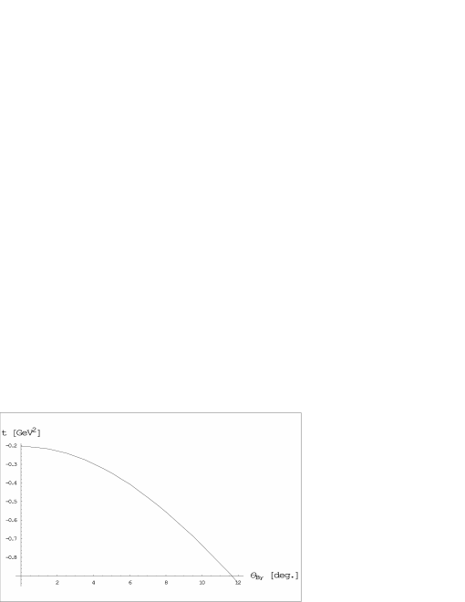As an example of the particular kinematics, we further choose $Q_{1}^{2}=2.5\;\mathrm{GeV}^{2},\;x_{B}=0.4$ and set $\varphi=0$. One plots t as a function of the angle $\theta_{B\gamma}$ between the incoming weak virtual boson B and the outgoing real photon $\gamma$ in the target rest frame (see Figure 9).

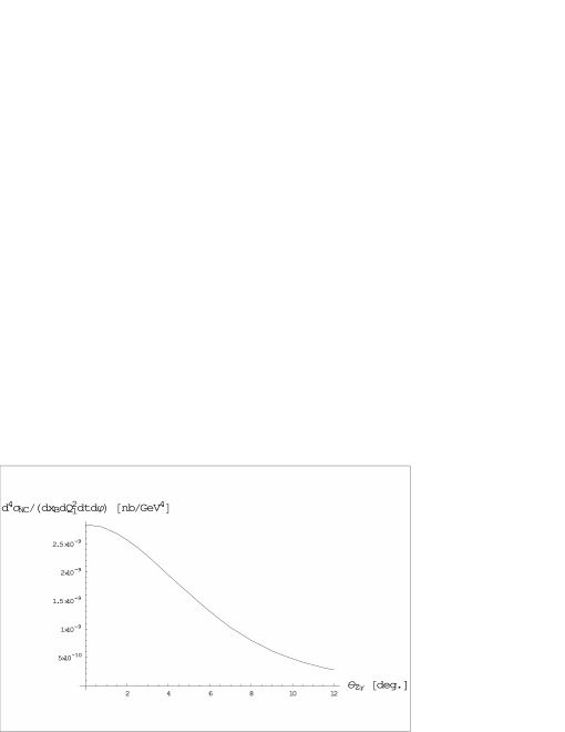
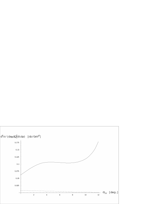
We study two different examples of the weak DVCS processes. In the weak neutral sector we consider neutrino scattering off an unpolarized proton target through the exchange of $Z^{0}$. Here one only measures the Compton contribution (see Figure 10) since the photon can not be emitted by the neutrino. Next we consider neutrino-neutron scattering through the exchange of $W^{+}$ with a proton in the final state. This particular process, however, has both contributions (see Figure 11). The Bethe-Heitler background is calculated from one diagram (see diagram (b) in Figure 7) since only the outgoing muon can emit the real photon. In contrast to the standard electromagnetic DVCS process on an unpolarized proton target (see Figure 12), where the Bethe-Heitler cross section is well above the Compton one, the situation in the weak charged sector is the other way round.

V Conclusions

Generalized parton distributions contain the most complete and unified description of the internal quark-gluon structure of hadrons. Form factors, usual parton distribution functions and distribution amplitudes, on the other hand, can be treated just as particular or limiting cases of generalized parton distributions. Furthermore, the formalism of generalized parton distributions provides nontrivial relations between exclusive and inclusive processes, and also between different exclusive processes.

We have extended the deeply virtual Compton scattering process into the weak sector by using the neutrino beam. We have argued that the weak deeply virtual Compton scattering process gives an additional information about the hadronic structure. It is expected in the near future that neutrino scattering off a nucleon will be studied at high intensity neutrino beam facilities.

VI Figures and Plots

Figure 1: Elastic electron-nucleon scattering in one-photon exchange approximation (left) and deeply inelastic scattering (right).

Figure 2: Optical theorem.

Figure 3: Forward virtual Compton scattering amplitude.

Figure 4: Non-forward virtual Compton scattering amplitude.

Figure 5: Symmetric description of the s-channel handbag diagram.

Figure 6: Handbag diagrams (s- and u-channel) in the weak DVCS amplitude.

Figure 7: DVCS (a) and Bethe-Heitler (b and c) diagrams contributing to the lepton-production of a real photon.

Figure 8: Kinematically allowed region.

Figure 9: Momentum transfer squared plotted as a function of the angle between the incoming weak virtual boson and outgoing real photon in the target rest frame.

Figure 10: Weak neutral DVCS differential cross section on an unpolarized proton target plotted as a function of the angle between the incoming weak virtual boson and outgoing real photon in the target rest frame.

Figure 11: Compton (dashed line) and Bethe-Heitler (solid line) contribution to the weak charged DVCS differential cross section on an unpolarized neutron target plotted as a function of the angle between the incoming weak virtual boson and outgoing real photon in the target rest frame.

Figure 12: Compton (dashed line) and Bethe-Heitler (solid line) contribution to the electromagnetic DVCS differential cross section on an unpolarized proton target plotted as a function of the angle between the incoming weak virtual boson and outgoing real photon in the target rest frame.

References

• (1) D. Muller, D. Robaschik, B. Geyer, F. M. Dittes and J. Horejsi, Fortsch. Phys.  42, 101 (1994) [arXiv:hep-ph/9812448].
• (2) X. D. Ji, Phys. Rev. Lett.  78, 610 (1997) [arXiv:hep-ph/9603249].
• (3) X. D. Ji, Phys. Rev. D 55, 7114 (1997) [arXiv:hep-ph/9609381].
• (4) A. V. Radyushkin, Phys. Lett. B 380, 417 (1996) [arXiv:hep-ph/9604317].
• (5) A. V. Radyushkin, Phys. Rev. D 56, 5524 (1997) [arXiv:hep-ph/9704207].
• (6) K. Goeke, M. V. Polyakov and M. Vanderhaeghen, Prog. Part. Nucl. Phys.  47, 401 (2001) [arXiv:hep-ph/0106012].
• (7) M. Diehl, Phys. Rept.  388, 41 (2003) [arXiv:hep-ph/0307382].
• (8) M. Burkardt, Phys. Rev. D 62, 071503 (2000) [Erratum-ibid. D 66, 119903 (2002)][arXiv:hep-ph/0005108].
• (9) P. A. M. Guichon and M. Vanderhaeghen, Prog. Part. Nucl. Phys.  41, 125 (1998) [arXiv:hep-ph/9806305].
• (10) A. V. Radyushkin, Phys. Rev. D 58, 114008 (1998) [arXiv:hep-ph/9803316].
• (11) A. V. Belitsky, D. Muller and A. Kirchner, Nucl. Phys. B 629, 323 (2002) [arXiv:hep-ph/0112108].
• (12) M. Goshtasbpour and G. P. Ramsey, Phys. Rev. D 55, 1244 (1997) [arXiv:hep-ph/9512250].
• (13) M. Penttinen, M. V. Polyakov and K. Goeke, Phys. Rev. D 62, 014024 (2000) [arXiv:hep-ph/9909489].