Consistency checks of pion-pion scattering data and chiral dispersive calculations

Abstract

We have evaluated forward dispersion relations for scattering amplitudes that follow from direct fits to several sets of $\pi\pi$ scattering experiments, together with the precise K decay results, and high to energy data. We find that some of the most commonly used experimental sets, as well as some recent theoretical analyses based on Roy equations, do not satisfy these constraints by several standard deviations. Finally, we provide a consistent $\pi\pi$ amplitude by improving a global fit to data with these dispersion relations.

1 Introduction

A precise knowledge of the $\pi\pi$ scattering amplitude has become increasingly important since it provides crucial tests for one and two loop Chiral Perturbation Theory (ChPT), as well as crucial information on three topics under intensive experimental and theoretical investigation: light meson spectroscopy, pionic atom decays and CP violation in kaons. Unfortunately, these precision studies are very cumbersome due to the poor quality of the data which is affected by large systematic errors. Here we review our recent work where we checked the fulfillment of dispersion relations by different sets of data commonly used in the literature, and provided parametrizations consistent with such requirements.

Recently, Ananthanarayan, Colangelo, Gasser and Leutwyler (ACGL)1 and Colangelo, Gasser and Leutwyler (CGL)2 have used data, analyticity and unitarity through Roy equations, and ChPT, to build a $\pi\pi$ amplitude. They provide phase shifts up to $0.8\,\mathop{\rm GeV}\nolimits$, scattering lengths and effective ranges claiming an outstanding precision. While the methods of CGL constitute a substantial improvement over previous ones, their analysis has to rely on some input, part of which we have recently questioned. First of all, their Regge high energy representation does not describe the high energy data, and does not satisfy well certain sum rules. Second, their D2 wave is incompatible with a number of requirements. Finally some of their input has remarkably small errors and relies precisely on some data sets that do not satisfy well forward dispersion relations. All this is discussed in the present note, which is based our recent works 3 ; 4 ; 5 .

2 Low Energy Partial waves from fits to data

2.1 The S0, S2 and P partial waves at low energy, $s^{1/2}\mathop{\hbox{$\displaystyle\raise 2.2pt\hbox{$\;<$}\kern-7.7pt\lower 2.6pt\hbox{$\sim$}\;$}}1\,\mathop{\rm GeV}\nolimits$

We first consider wave-by-wave fits to data for the S0, S2, P waves, as in 5 , which improve our “tentative solution” in 3 . To fit the phase shifts, $\delta(s)$, we parametrize $\cot\delta(s)$ taking into account its analytic properties, as well as its zeros (associated with resonances) and poles (when the phase shift crosses $n\pi$, $n=$integer).

For the P wave, up to $\simeq 1\,$GeV we use the results from a fit to the pion form factor as given in 6 . The comparison with $\pi\pi$ scattering data can be seen in Fig.1. We take $s_{0}$ as the point at which inelasticity begins to be nonegligible, and we write

$$\cot\delta_{1}(s)={\displaystyle{s^{1/2}\over 2k^{3}}}(M^{2}_{\rho}-s)\left\{B_{0}+B_{1}{\displaystyle{\sqrt{s}-\sqrt{s_{0}-s}\over\sqrt{s}+\sqrt{s_{0}-s}}}\right\};\quad s_{0}^{1/2}=1.05\;\mathop{\rm GeV}\nolimits.$$ (1)

$$B_{0}=\,1.069\pm 0.011,\quad B_{1}=0.13\pm 0.05,\quad M_{\rho}=773.6\pm 0.9,$$ (2)

$$a_{1}=\,(37.6\pm 1.1)\times 10^{-3}M_{\pi}^{-3},\quad b_{1}=(4.73\pm 0.26)\times 10^{-3}M_{\pi}^{-5};$$ (3)

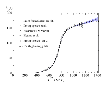
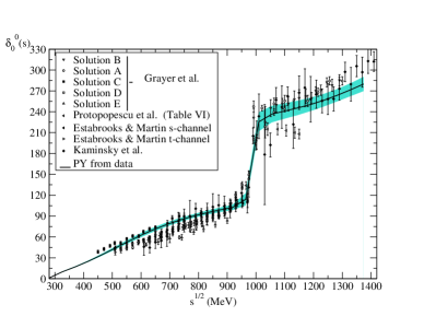
Figure 1: a) P wave phase shifts from $\pi\pi$ scattering 9 ; 10 compared with the prediction with the parameters (2.1) (solid line below 1 GeV). Note that this is not a fit to these data, but is obtained from the pion form factor 6 . The error here is like the thickness of the line. Above 1 GeV, the dotted line and error (PY) are as follows from the fit in 5 . b) S0 phase shifts and error band as given by Eqs.(7,8) below 1 GeV, and from 5 above. The $K_{l4}$ and $K_{2\pi}$ decay data are not shown. (see our 5 for details).

For the S2 wave we fit data where two like charge pions are produced:7 although these pions are not all on their mass shell, at least there is no problem of interference among various isospin states. At low energies, we fix the Adler zero at $z_{2}=M_{\pi}$ and fit only the low energy data, $s^{1/2}<1.0\,\mathop{\rm GeV}\nolimits$; later on we allow $z_{2}$ to vary. We have

$$\cot\delta_{0}^{(2)}(s)={\displaystyle{s^{1/2}\over 2k}}\,{\displaystyle{M_{\pi}^{2}\over s-2z_{2}^{2}}}\,\left\{B_{0}+B_{1}{\displaystyle{\sqrt{s}-\sqrt{s{{}_{0}}-s}\over\sqrt{s}+\sqrt{s{{}_{0}}-s}}}\right\},\quad s{{}_{0}}^{1/2}=1.05\;\mathop{\rm GeV}\nolimits,$$ (4)

$$B_{0}=\,-80.4\pm 2.8,\quad B_{1}=-73.6\pm 12.6;$$ (5)

$$a_{0}^{(2)}=\,(-0.052\pm 0.012)\,M_{\pi}^{-1};\quad b_{0}^{(2)}=(-0.085\pm 0.011)\,M_{\pi}^{-3}.$$ (6)

The S0 wave experimental situation is somewhat confusing, and we consider two methods of data selection. In both, we fit $K_{l4}$ and $K\to 2\pi$ decay data, in which pions are on the mass shell. In the first method, called global fit, we include some points at $0.81\,\mathop{\rm GeV}\nolimits\leq s^{1/2}\leq 0.97\,\mathop{\rm GeV}\nolimits$, where the various experiments agree within $\mathop{\hbox{$\displaystyle\raise 2.2pt\hbox{$\;<$}\kern-7.7pt\lower 2.6pt\hbox{$\sim$}\;$}}1.5\,\sigma$. Care is exercised to compose errors realistically, see details in 5 , Subsect 2.2.2. In this case we fix the Adler zero at $z_{0}=M_{\pi}$ and find

$$\cot\delta_{0}^{(0)}(s)=\,{\displaystyle{s^{1/2}\over 2k}}\,{\displaystyle{M_{\pi}^{2}\over s-{\textstyle{1\over 2}}z_{0}^{2}}}\,{\displaystyle{M^{2}_{\sigma}-s\over M^{2}_{\sigma}}}\,\left\{B_{0}+B_{1}{\displaystyle{\sqrt{s}-\sqrt{s_{0}-s}\over\sqrt{s}+\sqrt{s_{0}-s}}}\right\},$$ (7)

$${B}_{0}=\,21.04,\quad{B}_{1}=6.62,\quad M_{\sigma}=782\pm 24\,\mathop{\rm MeV}\nolimits;\quad\delta_{0}^{(0)}(m_{K})=41.0{{}^{\circ}\,}\pm 2.1{{}^{\circ}\,};$$

$$a_{0}^{(0)}=\,(0.230\pm 0.010)M_{\pi}^{-1},\quad b_{0}^{(0)}=(0.268\pm 0.011)M_{\pi}^{-3};$$

this fit (shown in Fig 1.b as PY) is valid for $s^{1/2}\leq 0.95\,\mathop{\rm GeV}\nolimits$. The $B_{i}$ errors are strongly correlated; uncorrelated errors are obtained if using the parameters $x,\,y$ with

$$B_{0}=y-x;\quad B_{1}=6.62-2.59x;\quad y=21.04\pm 0.70,\quad x=0\pm 2.6.$$ (8)

The other method is to fit only $K_{l4}$ and $K\to 2\pi$ data, or to add to this, individually, data from the various experimental analyses. The results can be found in Table 1.

2.2 The S0, S2 and P partial waves at $1\,\mathop{\rm GeV}\nolimits\mathop{\hbox{$\displaystyle\raise 2.2pt\hbox{$\;<$}\kern-7.7pt\lower 2.6pt\hbox{$\sim$}\;$}}s^{1/2}\mathop{\hbox{$\displaystyle\raise 2.2pt\hbox{$\;<$}\kern-7.7pt\lower 2.6pt\hbox{$\sim$}\;$}}1.42\,\mathop{\rm GeV}\nolimits$

The D and F data are scanty, and have large errors. To stabilize the fits we impose the values of the scattering lengths that follow from the Froissart–Gribov representation. This is not circular reasoning since their Froissart–Gribov representation depends mostly on the S0, S2 and P waves, and very little on the D0, D2, F waves themselves. We do not discuss here the D0 and F waves (see 5 ) as they do not present special features.

For D2 we only expect important inelasticity when the $\pi\pi\to\rho\rho$ channel opens up, so that $s_{0}=1.45^{2}\,\mathop{\rm GeV}\nolimits^{2}\sim 4M^{2}_{\rho}$. A pole term is necessary here, since we expect $\delta_{2}^{(2)}$ to change sign near threshold: the data 7 give negative and small values for $\delta^{(2)}_{2}$ above some $500\,\mathop{\rm MeV}\nolimits$, while, from the Froissart–Gribov representation, it is known12 that the scattering length must be positive. Indeed we include in the fit the value $a_{2}^{(2)}=(2.72\pm 0.36)\times 10^{-4}\,M_{\pi}^{-5}$. In addition, the clear inflection seen in data around 1 GeV asks for a third order conformal expansion. So we write

$$\cot\delta_{2}^{(2)}(s)={\displaystyle{s^{1/2}\over 2k^{5}}}\,\Big{\{}B_{0}+B_{1}w(s)+B_{2}w(s)^{2}\Big{\}}\,{\displaystyle{{M_{\pi}}^{4}s\over 4({M_{\pi}}^{2}+\Delta^{2})-s}},\;w(s)={\displaystyle{\sqrt{s}-\sqrt{s_{0}-s}\over\sqrt{s}+\sqrt{s_{0}-s}}}.$$

And we find $B_{0}=(2.4\pm 0.3)\times 10^{3}$, $B_{1}=(7.8\pm 0.8)\times 10^{3}$, $B_{2}=(23.7\pm 3.8)\times 10^{3}$, $\Delta=196\pm 20\,\mathop{\rm MeV}\nolimits$.

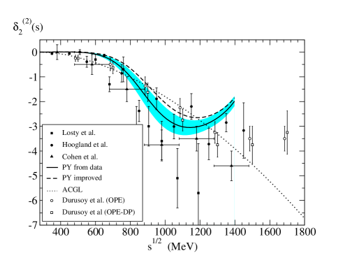
Figure 2: Continuous line: The $I=2$, $D$-wave phase shift, obtained by only fitting the experimental data. Broken line: with the parameters improved using dispersion relations. Dotted line: the fit, valid between $s^{1/2}=0.625\,\mathop{\rm GeV}\nolimits$ and 1.375 GeV, of Martin, Morgan and Shaw which ACGL and CGL, however, use from threshold to $s^{1/2}=2\,\mathop{\rm GeV}\nolimits$. The experimental points are from 7 .

The fit, which may be found in Fig 2, returns reasonable numbers for the scattering length and for the effective range parameter, $b_{2}^{(2)}$:

$$a_{2}^{(2)}=(2.5\pm 0.9)\times 10^{-4}\,{M_{\pi}}^{-5};\quad b_{2}^{(2)}=(-2.7\pm 0.8)\times 10^{-4}\,{M_{\pi}}^{-7}.$$ (9)

3 The high energy ($s^{1/2}\geq 1.42\,\mathop{\rm GeV}\nolimits$) input

In order to test dispersion relations we also need the imaginary part of the scattering amplitude at $s^{1/2}\geq 1.42\;\mathop{\rm GeV}\nolimits$, that we take from a Regge fit to data 4 (and the slightly improved rho residue of 5 ). We note that, in the early 1970s, when $\pi\pi$ phase shifts were poorly known and, above all, when it was still not clear that the standard Regge picture is a QCD feature, Regge factorization was questioned 13 using crossing sum rules and then-existing low energy phase shift data. This was adopted later by ACGL and CGL, assuming a too large rho residue and a Pomeron a third of what factorization and the experimental data on the total $\pi\pi$ cross section implies, as well as unconventional slopes. Unfortunately this has been also used in subsequent Roy equation analyses. As discussed in 4 ; 5 , however, standard Regge factorization describes experiment 14 ; Pelaez:2004ab and is perfectly consistent with crossing sum rules if assumed to hold above $1.42\;\mathop{\rm GeV}\nolimits$.

In Fig 3 we show our Regge description of the imaginary parts of $\pi\pi$ scattering amplitudes 4 ; 5 ; Pelaez:2004ab together with the data14 , compared with that used by ACGL1 , CGL2 above 2 GeV.

Between $1.42\,\mathop{\rm GeV}\nolimits\leq s^{1/2}\leq 2\,\mathop{\rm GeV}\nolimits$, these authors use the scattering amplitude reconstructed from one Cern–Munich phase shift analysis, and, in particular for S0, the re-elaboration of Au, Morgan and Pennington 10 . Unfortunately, in this region the inelasticity is large and the Cern–Munich experiments, which only measure the differential cross section for $\pi\pi\to\pi\pi$ are insufficient to reconstruct without ambiguity the full imaginary part. In addition, in 3 ; 5 we showed that Cern–Munich phases fail to pass a number of consistency tests. This is also seen clearly in Fig 3, where we plot the total cross section for $\pi^{+}\pi^{-}$ that follows Hyams et al.,10 , which is incompatible with other experimental data 14 , as well as with Regge factorization.

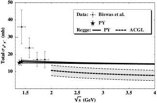
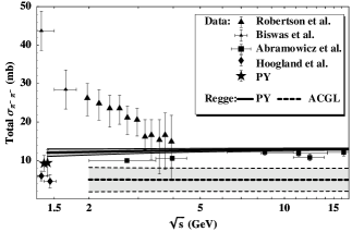
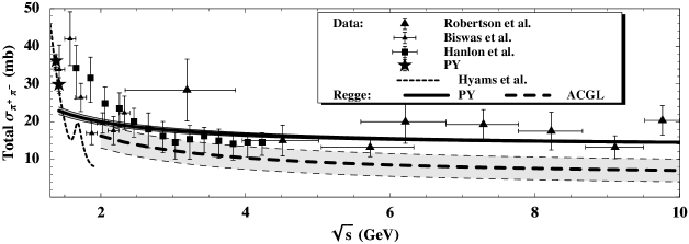
Figure 3: The $\pi\pi$ cross sections. Experimental points from 14 . The stars at 1.38 and 1.42 GeV (PY) are from the phase shift analysis of experimental data given in 5 . Continuous lines, from 1.42 GeV (PY): Regge formula, with parameters as in 4 (the three lines per fit cover the error in the theoretical values of the Regge residues). Dashed lines, above 2 GeV: the cross sections following from ACGL;1 the gray band covers their error band. Below 2 GeV, the dotted line corresponds to the $\pi^{+}\pi^{-}$ cross section from the Cern–Munich analysis; cf. Fig 7 in the paper of Hyams et al.10

In a recent paper Caprini, Colangelo, Gasser and Leutwyler,20 to be denoted by CCGL, review our work in 3 and conclude that, still, they consider the CGL solution consistent. They also raised the contention that our Reggeistics could not be correct because it violates certain sum rules. In view of Fig.3 this contention is meaningless since the PY cross sections are perfectly compatible with high energy ($s^{1/2}\geq 1.42\mathop{\rm GeV}\nolimits$) experimental data, while the ACGL ones are not. In 3 ; 4 ; 5 we also checked that our representation satisfies two crossing sum rules.

Concerning D2, ACGL and CGL borrow an old fit in the book of Martin, Morgan and Shaw,15 where only intermediate energy data were fitted.

$$\delta_{2}^{(2)}(s)=-0.003(s/4M^{2}_{\pi})\left(1-4M^{2}_{\pi}/s\right)^{5/2},$$ (10)

which fails at threshold (it gives a negative scattering length) and does not fit well data below 1.42 GeV, as shown in Fig 2. Above 1 GeV, this D2 phase grows quadratically with the energy, while Regge theory predicts all phases to go to a multiple of $\pi$. In particular D2 should go to zero; see Appendix C of 5 for details. It is true that this D2 wave is small but, given the accuracy claimed by CGL, it is certainly not negligible.

4 Checking forward dispersion relations

In the present Section we study how well the previous amplitudes obtained from fits to different sets of data satisfy forward dispersion relations. We consider three independent scattering amplitudes in $t$-symmetric or antisymmetric combinations, that form a complete set: $\pi^{0}\pi^{0}\to\pi^{0}\pi^{0}$, $\pi^{0}\pi^{+}\to\pi^{0}\pi^{+}$, and the $t$ channel isospin one amplitude, $I_{t}=1$. The reason is that the two first depend only on two isospin states, and have positivity properties: their imaginary parts are sums of positive terms, thus reducing the final uncertainties. Hence, for $\pi^{0}\pi^{0}$, we have

$$\mathop{\rm Re}F_{00}(s)-F_{00}(4M_{\pi}^{2})={\displaystyle{s(s-4M_{\pi}^{2})\over\pi}}\mathop{\rm P.P.}\int_{4M_{\pi}^{2}}^{\infty}{\rm d}s^{\prime}\,{\displaystyle{(2s^{\prime}-4M^{2}_{\pi})\mathop{\rm Im}F_{00}(s^{\prime})\over s^{\prime}(s^{\prime}-s)(s^{\prime}-4M_{\pi}^{2})(s^{\prime}+s-4M_{\pi}^{2})}}.$$ (11)

In particular, for $s=2M^{2}_{\pi}$, which will be important for the Adler zeros, we have

$$F_{00}(4M_{\pi}^{2})=F_{00}(2M_{\pi}^{2})+D_{00},\quad D_{00}={\displaystyle{8M_{\pi}^{4}\over\pi}}\int_{4M_{\pi}^{2}}^{\infty}{\rm d}s\,{\displaystyle{\mathop{\rm Im}F_{00}(s)\over s(s-2M_{\pi}^{2})(s-4M_{\pi}^{2})}}.$$ (12)

For the $\pi^{0}\pi^{+}$ channel, which does not depend on S0:

$$\mathop{\rm Re}F_{0+}(s)-F_{0+}(4M_{\pi}^{2})={\displaystyle{s(s-4M^{2}_{\pi})\over\pi}}\mathop{\rm P.P.}\int_{4M_{\pi}^{2}}^{\infty}{\rm d}s^{\prime}\,{\displaystyle{(2s^{\prime}-4M^{2}_{\pi})\mathop{\rm Im}F_{0+}(s^{\prime})\over s^{\prime}(s^{\prime}-s)(s^{\prime}-4M_{\pi}^{2})(s^{\prime}+s-4M_{\pi}^{2})}}.$$

At the point $s=2M^{2}_{\pi}$, this becomes

$$F_{0+}(4M_{\pi}^{2})=F_{0+}(2M_{\pi}^{2})+D_{0+},\quad D_{0+}={\displaystyle{8M_{\pi}^{4}\over\pi}}\int_{8M_{\pi}^{2}}^{\infty}{\rm d}s\,{\displaystyle{\mathop{\rm Im}F_{0+}(s)\over s(s-2M_{\pi}^{2})(s-4M_{\pi}^{2})}}.$$ (13)

Finally, for isospin unit exchange, which does not require subtractions,

$$\mathop{\rm Re}F^{(I_{t}=1)}(s,0)={\displaystyle{2s-4M^{2}_{\pi}\over\pi}}\,\mathop{\rm P.P.}\int_{4M^{2}_{\pi}}^{\infty}{\rm d}s^{\prime}\,{\displaystyle{\mathop{\rm Im}F^{(I_{t}=1)}(s^{\prime},0)\over(s^{\prime}-s)(s^{\prime}+s-4M^{2}_{\pi})}}.$$ (14)

at threshold this is known as the Olsson sum rule.

Depending on the method we use to fit the S0 wave we find the results in Table 1, where, we have separated on top those fits to data with a total $\chi^{2}/d.o.f.<6$ for the $\pi^{0}\pi^{0}$ and $I_{t}=1$ dispersion relations up to 0.925 GeV, a fairly reasonable $\chi^{2}/d.o.f.$ since these fits were obtained independently of the dispersive approach.

	$B_{0}$	$B_{1}$	$M_{\sigma}$ (MeV)	${I_{t}=1}\atop{{\displaystyle{\chi^{2}\over\rm d.o.f.}}}$	${\pi^{0}\pi^{0}}\atop{{\displaystyle{\chi^{2}\over\rm d.o.f.}}}$	$\delta_{0}^{(0)}(0.8^{2})$
PY, Eqs.(7,8)	$21.04$	$6.62$	$782\pm 24$	$0.3$	$3.5$	$91.9{{}^{\circ}\,}$
$K\;{\rm decay\;only}$	$\phantom{\Big{|}}18.5\pm 1.7$	$\equiv 0$	$766\pm 95$	$0.2$	$1.8$	$93.2{{}^{\circ}\,}$
${\displaystyle{{K\;{\rm decay\;data}}}\atop{\displaystyle+\,{\rm Grayer,\;B}}}$	$22.7\pm 1.6$	$12.3\pm 3.7$	$858\pm 15$	$1.0$	$2.7$	$84.0{{}^{\circ}\,}$
${\displaystyle{{K\;{\rm decay\;data}}}\atop{\displaystyle+\,{\rm Grayer,\;C}}}$	$16.8\pm 0.85$	$-0.34\pm 2.34$	$787\pm 9$	$0.4$	$1.0$	$91.1{{}^{\circ}\,}$
${\displaystyle{{K\;{\rm decay\;data}}}\atop{\displaystyle+\,{\rm Grayer,\;E}}}$	$21.5\pm 3.6$	$12.5\pm 7.6$	$1084\pm 110$	$2.1$	$0.5$	$70.6{{}^{\circ}\,}$
${\displaystyle{{K\;{\rm decay\;data}}}\atop{\displaystyle+\,{\rm Kaminski}}}$	$27.5\pm 3.0$	$21.5\pm 7.4$	$789\pm 18$	$0.3$	$5.0$	$91.6{{}^{\circ}\,}$
${\displaystyle{{K\;{\rm decay\;data}}}\atop{\displaystyle+\,{\rm Grayer,\;A}}}$	$28.1\pm 1.1$	$26.4\pm 2.8$	$866\pm 6$	$2.0$	$7.9$	$81.2{{}^{\circ}\,}$
${\displaystyle{{K\;{\rm decay\;data}}}\atop{\displaystyle+\,{{\rm EM},\;s{\rm-channel}}}}$	$29.8\pm 1.3$	$25.1\pm 3.3$	$811\pm 7$	$1.0$	$9.1$	$88.3{{}^{\circ}\,}$
${\displaystyle{{K\;{\rm decay\;data}}}\atop{\displaystyle+\,{{\rm EM},\;t{\rm-channel}}}}$	$29.3\pm 1.4$	$26.9\pm 3.4$	$829\pm 6$	$1.2$	$10.1$	$85.7{{}^{\circ}\,}$
${\displaystyle{{K\;{\rm decay\;data}}}\atop{\displaystyle+\,{\rm Protopopescu\,VI}}}$	$27.0\pm 1.7$	$22.0\pm 4.1$	$855\pm 10$	$1.2$	$5.8$	$82.9{{}^{\circ}\,}$
${\displaystyle{{K\;{\rm decay\;data}}}\atop{\displaystyle+\,{\rm Protopopescu\,XII}}}$	$25.5\pm 1.7$	$18.5\pm 4.1$	$866\pm 14$	$1.2$	$6.3$	$82.2{{}^{\circ}\,}$
${\displaystyle{{K\;{\rm decay\;data}}}\atop{\displaystyle+\,{\rm Protopopescu\,3}}}$	$27.1\pm 2.3$	$23.8\pm 5.0$	$913\pm 18$	$1.8$	$4.2$	$76.7{{}^{\circ}\,}$

Table 1: PY: our global fit, Eqs.(7,8). We do not give its $B_{0}$ and $B_{1}$ uncertainties as they are strongly correlated, see Eq.(8) for the uncorrelated ones. Grayer B, C, E: different solutions in Grayer et al.10 . Kaminski: 10 . In 5 we have also studied fits to the data in Tables VI, XII and VIII in 9 , to Solution A in10 , as well as fits to the theoretical outcome in Estabrooks and Martin.10 . They all give a total $\chi^{/}{\rm d.o.f.}\geq 6$

However, in Table 1 we also list the very frequently used $t$ and $s$-channel solutions of Estabrooks and Martin 10 , those of Protopopescu et al.9 , from Table VI, VIII and table XII, as well as the solution A of Grayer et al. 10 . Their $I_{t}=1$ plus $\pi^{0}\pi^{0}$ dispersion relation total $\chi^{2}/d.o.f.$ is surprisingly poor: 11.3, 10.1, 7, 6, 7.5, 9.9, respectively. Therefore, any result that relies heavily on these sets should be taken very cautiously.

5 Improved fits using dispersion relations

We now improve the previous low energy fits parameters by fitting also the dispersion relations up to 0.925 GeV, thus obtaining parametrizations more compatible with analyticity and $s\,-\,u$ crossing. This is an alternative method to Roy equations; it is better in that we do not need as input the scattering amplitude for $|t|$ up to $30M^{2}_{\pi}$, where the Regge fits existing in the literature disagree strongly (see 5 , Appendix B) and also in that we can test all energies5 , whereas Roy equations are valid for $s^{1/2}<\sqrt{60}\,M_{\pi}\sim 1.1\,\mathop{\rm GeV}\nolimits$ (and only applied up to $0.8\,\mathop{\rm GeV}\nolimits$). Starting from Eqs.(7,8), we find, in $M_{\pi}$ units,

$${\rm S0};\;s^{1/2}\leq 2m_{K}: B_{0}=17.4\pm 0.5;\;B_{1}=4.3\pm 1.4;$$ (17)

$$M_{\sigma}=790\pm 21\,\mathop{\rm MeV}\nolimits;\;z_{0}=195\,\mathop{\rm MeV}\nolimits\;\hbox{[Fixed]};$$

$$a_{0}^{(0)}=0.230\pm 0.015;\;b_{0}^{(0)}=0.312\pm 0.014.$$

$${\rm S2};\;s^{1/2}\leq 1.0: B_{0}=-80.8\pm 1.7;\;B_{1}=-77\pm 5;\;z_{2}=147\,\mathop{\rm MeV}\nolimits\;\hbox{[Fixed]};$$ (19)

$$a_{0}^{(2)}=-0.0480\pm 0.0046;\;b_{0}^{(2)}=-0.090\pm 0.006.$$

$${\rm S2};\;1.0\leq s^{1/2}\leq 1.42: B_{0}=-125\pm 6;\;B_{1}=-119\pm 14;\;\epsilon=0.17\pm 0.12.$$ (20)

$${\rm P};\;s^{1/2}\leq 1.05: B_{0}=1.064\pm 0.11;\;B_{1}=0.170\pm 0.040;\;M_{\rho}=773.6\pm 0.9\;\mathop{\rm MeV}\nolimits;$$ (22)

$$a_{1}=(38.7\pm 1.0)\times 10^{-3};\;b_{1}=(4.55\pm 0.21)\times 10^{-3}.$$

$${\rm D0};\;s^{1/2}\leq 1.42: B_{0}=23.5\pm 0.7;\;B_{1}=24.8\pm 1.0;\;\epsilon=0.262\pm 0.030;$$ (24)

$$\;a_{2}^{(0)}=(18.4\pm 3.0)\times 10^{-4};\;b_{2}^{(0)}=(-8.6\pm 3.4)\times 10^{-4}.$$

$${\rm D2};\;s^{1/2}\leq 1.42: B_{0}=(2.9\pm 0.2)\times 10^{3};\;B_{1}=(7.3\pm 0.8)\times 10^{3};\;$$ (27)

$$B_{2}=(25.4\pm 3.6)\times 10^{3};\;\Delta=212\pm 19;$$

$$a_{2}^{(2)}=(2.4\pm 0.7)\times 10^{-4};\;b_{2}^{(2)}=(-2.5\pm 0.6)\times 10^{-4}.$$

$${\rm F};\;s^{1/2}\leq 1.42: B_{0}=(1.09\pm 0.03)\times 10^{5};\;B_{1}=(1.41\pm 0.04)\times 10^{5};$$ (28)

$$a_{3}=(7.0\pm 0.8)\times 10^{-5}.$$

In Fig.4 we show the improved curves for S0 and S2, and that of D2 in Fig.2.

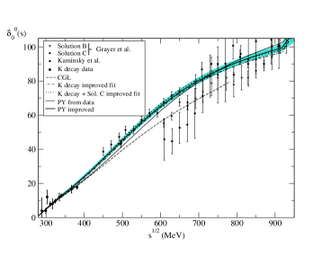
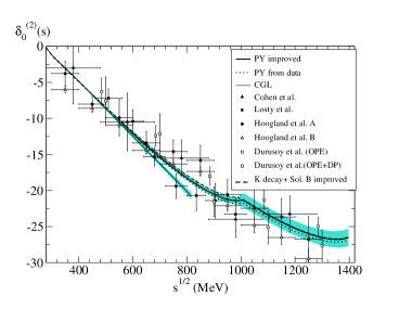
Figure 4: a) The improved S0 phase shift (PY improved, Eq.28), the global fit (PY from data, he S0 Eqs. (7,8)), and the improved solutions “$K$ decay only” and “Grayer C” of Table 2 (almost on top of PY improved). The solution CGL2 (dashed line) is also shown. b) S2 improved Phase shift (PY improved, Eq. (28)); global fit (PY from data, Eq. (6)); the solution CGL 2 (thin continuous line) and the improved parametrization with K decays and So. B of Grayer et al.10 .

Concerning the improved fits to individual sets of data, we get somewhat different results for S0, listed in Table 2. In Table 2 we also show the $\chi^{2}/d.o.f.$ of each forward dispersion relation and the standard deviations for the sum rule in Eq.12, which are more than four for K decay plus the Grayer B or E or Kaminski improved solutions. Concerning the other waves, no matter what set of parameters from data fits we start from, we end up with very similar values to those given in Eq.28. This can be checked in Fig.4.b, where we show the improved “K decay + Grayer Sol. B” S2 wave. Even though it is the one for which we obtained the most different central values for the S0 wave compared with those given in Eq.28, it falls perfectly within the uncertainty of our improved solution.

Table 2: Improved fits. Names are as in Table 1. Although errors are given for the Adler zero, we fix it when evaluating other errors, to break the otherwise very large correlations

Improved	Improved	$K$ decay only	$K$ decay	$K$ decay	$K$ decay	$K$ decay
fits:	PY, Eq.28		+grayer C	+Grayer B	+Grayer E	+ Kamiński
$B_{0}$	$17.4\pm 0.5$	$16.4\pm 0.9$	$16.2\pm 0.7$	$20.7\pm 1.0$	$20.2\pm 2.2$	$20.8\pm 1.4$
$B_{1}$	$4.3\pm 1.4$	$\equiv 0$	$0.5\pm 1.8$	$11.6\pm 2.6$	$8.4\pm 5.2$	$13.6\pm 43.7$
$M_{\sigma}\,$(MeV)	$790\pm 30$	$809\pm 53$	$788\pm 9$	$861\pm 14$	$982\pm 95$	$798\pm 17$
$z_{0}\,$(MeV)	$195\pm 30$	$182\pm 34$	$182\pm 39$	$233\pm 30$	$272\pm 50$	$245\pm 39$
${\displaystyle I_{t}=1}\atop{\chi^{2}/d.o.f.}$	0.40	0.30	0.37	0.37	0.60	0.43
${\displaystyle\pi^{0}\pi^{0}}\atop{\chi^{2}/d.o.f.}$	0.66	0.29	0.32	0.83	0.09	1.08
${\displaystyle\pi^{+}\pi^{-}}\atop{\chi^{2}/d.o.f.}$	1.62	1.77	1.74	1.60	1.40	1.36
Eq.(12)	1.6$\sigma$	1.5$\sigma$	1.5$\sigma$	4.0$\sigma$	6.0$\sigma$	4.5$\sigma$
$\delta^{(0)}_{0}(0.8^{2}{\rm GeV}^{2})$	91.3∘	91.3∘	91.0∘	85.1∘	78.0∘	91.8∘

6 Dispersion relations and the CGL solution

We have also checked the fulfillment of forward dispersion relations for the CGL solution for the S0, S2 and P waves al low energy. This is depicted in Fig 5, where we show, both for CGL and our improved fit, Eq.(28), the mismatch between the real part and the dispersive evaluations, that is to say, the differences $\Delta_{i}$,

$$\Delta_{1}\equiv\mathop{\rm Re}F^{(I_{t}=1)}(s,0)-{\displaystyle{2s-4M^{2}_{\pi}\over\pi}}\mathop{\rm P.P.}\int_{4M^{2}_{\pi}}^{\infty}{\rm d}s^{\prime}\,{\displaystyle{\mathop{\rm Im}F^{(I_{t}=1)}(s^{\prime},0)\over(s^{\prime}-s)(s^{\prime}+s-4M^{2}_{\pi})}},$$ (29)

$$\Delta_{00}\equiv\mathop{\rm Re}F_{00}(s)-F_{00}(4M_{\pi}^{2})$$ (30)

$$\qquad\quad-{\displaystyle{s(s-4M_{\pi}^{2})\over\pi}}\mathop{\rm P.P.}\int_{4M_{\pi}^{2}}^{\infty}{\rm d}s^{\prime}\,{\displaystyle{(2s^{\prime}-4M^{2}_{\pi})\mathop{\rm Im}F_{00}(s^{\prime})\over s^{\prime}(s^{\prime}-s)(s^{\prime}-4M_{\pi}^{2})(s^{\prime}+s-4M_{\pi}^{2})}},$$

$$\Delta_{0+}\equiv\mathop{\rm Re}F_{0+}(s)-F_{0+}(4M_{\pi}^{2})$$ (31)

$$\qquad\quad-{\displaystyle{s(s-4M^{2}_{\pi})\over\pi}}\mathop{\rm P.P.}\int_{4M_{\pi}^{2}}^{\infty}{\rm d}s^{\prime}\,{\displaystyle{(2s^{\prime}-4M^{2}_{\pi})\mathop{\rm Im}F_{0+}(s^{\prime})\over s^{\prime}(s^{\prime}-s)(s^{\prime}-4M_{\pi}^{2})(s^{\prime}+s-4M_{\pi}^{2})}}.$$

These quantities would vanish, $\Delta_{i}=0$, if the dispersion relations were exactly satisfied.

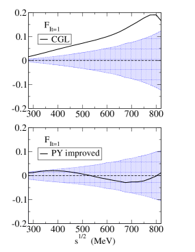
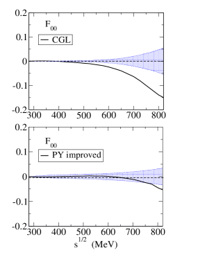
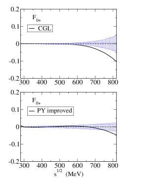
Figure 5: Dispersion relations for the $\pi\pi$ amplitudes of 2  (CGL) and for our improved global fit (PY improved, Eq.28. We plot the differences $\Delta_{i}$, Eqs. 29, between real parts calculated directly from the parametrizations, or from the dispersive formulas. Consistency within one sigma occurs within the shaded bands. The progressive deterioration of the CGL results as the energy increases is apparent here.

We include in the comparison of Fig 5 the uncertainties; in the case of CGL, these errors are as follow from the parametrizations given by these authors in 2 , for $s^{1/2}\mathop{\hbox{$\displaystyle\raise 2.2pt\hbox{$\;<$}\kern-7.7pt\lower 2.6pt\hbox{$\sim$}\;$}}0.8\,\mathop{\rm GeV}\nolimits$. At higher energies they are taken from data via our parametrizations. It can be clearly seen that the CGL parametrizations do not satisfy these forward dispersion relations by several standard deviations.

One might wonder why in Table 2, the S0 wave improved “K decay+solution B” yields $\chi^{2}/d.o.f.$ of order one for the forward dispersion relations, being so similar to what CGL get for that wave. The reason is that, as we show in Fig.4.b. the improved solution B, requires an S2 wave that is even farther from the CGL S2 wave than our global improved solution.

7 Low energy parameters in the literature

We here present, in Table 3, the low energy parameters obtained from Roy equations by CGL, by Descotes et al.15 , that we denote by DFGS, and by Kamiński, Leśniak and Loiseau15 , denoted by KLL. This is compared with what we find fitting experimental data, improved with dispersion relations (see 5 for details).

The mismatches between many of the parameters of CGL and PY are apparent here; not surprisingly, they affect mostly parameters sensitive to high energy:

• The S wave parameters are compatible, mainly due to the large PY uncertainties.

• The mismatch between CGL and PY for $a_{2}^{(I)}$ and $b_{2}^{(I)}$ is roughly $2.5\sigma$. In ref.3 we pointed out that the ACGL and CGL results did not satisfy the Froissart Gribov sum rules. This happens to more than four standard deviations for the difference between the CGL calculation using Wanders sum rules minus the Froissart-Gribov representation. This larger mismatch, as pointed out in 20 , does not involve the S and P waves, and is due to the Regge and $L\geq 2$ wave input, evidently very different from the beginning for CGL and PY, but that certainly affects the values of $a_{2}^{(I)}$ and $b_{2}^{(I)}$.

• The $b_{1}$ calculation differs by more than 4 standard deviations for PY and CGL.

	DFGS	KLL	CGL	PY
$a_{0}^{(0)}$	$0.228\pm 0.032$	$0.224\pm 0.013$	$0.220\pm 0.005$	$0.230\pm 0.015$
$a_{0}^{(2)}$	$-0.0382\pm 0.0038$	$-0.0343\pm 0.0036$	$-0.0444\pm 0.0010$	$-0.0480\pm 0.0046$
$b_{0}^{(0)}$		$0.252\pm 0.011$	$0.280\pm 0.001$	$0.312\pm 0.014$
$b_{0}^{(2)}$		$-0.075\pm 0.015$	$-0.080\pm 0.001$	$-0.090\pm 0.006$
$a_{1}\times 10^{3}$		$39.6\pm 2.4$	${\displaystyle 37.9\pm 0.5}$	$38.4\pm 0.8$
$b_{1}\times 10^{3}$		$2.83\pm 0.67$	$5.67\pm 0.13$	$4.75\pm 0.16$
$a_{2}^{(0)}\times 10^{4}$			$17.5\pm 0.3$	$18.70\pm 0.41$
$a_{2}^{(2)}\times 10^{4}$			$1.70\pm 0.13$	$2.78\pm 0.37$
$b_{2}^{(0)}\times 10^{4}$			$-3.55\pm 0.14$	$-4.16\pm 0.30$
$b_{2}^{(2)}\times 10^{4}$			$-3.26\pm 0.12$	$-3.89\pm 0.28$
$a_{3}\times 10^{5}$			$5.6\pm 0.2$	$6.3\pm 0.4$

Table 3: Units of $M_{\pi}$. The numbers in the CGL column are as given by CGL in Table 2 and elsewhere in their text. In PY, the values for the D, F waves parameters are from the Froissart–Gribov representation. The rest are from the fits, improved with dispersion relations, except for $a_{1}$ and $b_{1}$ that have been taken as in 5 .

8 The ACGL, CGL phase at $s^{1/2}=0.8\,$GeV

In the ACGL, CGL analyses, by the input phases for the S0, S2 and P waves at the point, $s^{1/2}=0.8\,\mathop{\rm GeV}\nolimits$, where they match the solutions to the Roy equations to the experimental amplitude. Indeed it is dominant for their Olsson sum rule calculation, which involves the $I_{t}=1$ channel.

The quantity $\delta_{0}^{(0)}((0.8\,\mathop{\rm GeV}\nolimits)^{2})$ is in fact given in Eq. (7.3) of ACGL as

$$\delta_{0}^{(0)}((0.8\,\mathop{\rm GeV}\nolimits)^{2})=82.3\pm 3.4{{}^{\circ}\,}.$$ (32)

whose error may be contrasted with the estimates of 5 , which vary, for the data above 0.8 GeV, between 6^∘ and 18^∘, or with the $\delta_{0}^{(0)}((0.8\,\mathop{\rm GeV}\nolimits)^{2})$ values we obtain from fits to different sets of data in Table 1, or the improved fits in Table 2. Small errors could be expected from theoretical analysis including many data but the above small error was used as an input.

The reason to consider such an small error is that ACGL consider the difference $\delta_{1}-\delta_{0}^{(0)}$ at 0.8 GeV, in the hope that some of the uncertainties will cancel. Then they interpolate and then average the points from a choice of three analysis of the CERN/Munich experiment10

$$\delta_{1}((0.8\,\mathop{\rm GeV}\nolimits)^{2})-\delta_{0}^{(0)}((0.8\,\mathop{\rm GeV}\nolimits)^{2})=\cases{23.4\pm 4.0{{}^{\circ}\,}\;\hbox{[Hyams et al.]}\cr 24.8\pm 3.8{{}^{\circ}\,}\;\hbox{[Estabrooks and Martin, $s$-channel]}\cr 30.3\pm 3.4{{}^{\circ}\,}\;\hbox{[Estabrooks and Martin, $t$-channel]}.\cr}$$

and set

$$\delta_{0}^{(0)}((0.8\,\mathop{\rm GeV}\nolimits)^{2})-\delta_{1}((0.8\,\mathop{\rm GeV}\nolimits)^{2})=26.6\pm 2.8{{}^{\circ}\,}.$$

However, this error does not include systematics. All numbers here stem from the same experiment, and differ only on the method of analysis. Their spread is an indication of the systematic uncertainties, roughly an additional $\pm 4{{}^{\circ}\,}$. In addition, the Hyams et al. value above is only one of five solutions in Grayer et al.10 , and considering also data of Protopopescu et al.,9 the systematic error would increase to $10{{}^{\circ}\,}$. Remarkably, Estabrooks and Martin themselves, point out in their section 4 (first paragraph) that different D wave input “lead to systematic changes in $\delta_{S}^{0}$ of the order of 10^∘”.

References

- (1) Ananthanarayan, B., Colangelo, G., Gasser, J., and Leutwyler, H., Phys. Rep., 353, 207, (2001).
- (2) Colangelo, G., Gasser, J., and Leutwyler, H., Nucl. Phys. B603, 125, (2001).
- (3) Peláez, J. R., and Ynduráin, F. J., Phys. Rev. D68, 074005 (2003).
- (4) Peláez, J. R., and Ynduráin, F. J., Phys. Rev. D69, 114001 (2004).
- (5) Peláez, J. R., and Ynduráin, F. J., FTUAM 04-14 hep-ph/0411334.
- (6) de Trocóniz, J. F., and Ynduráin, F. J., Phys. Rev., D65, 093001, (2002) and hep-ph/0402285. When quoting numbers, we will quote from this last paper.
- (7) Losty, M. J., et al. Nucl. Phys., B69, 185 (1974); Hoogland, W., et al. Nucl. Phys., B126, 109 (1977); Cohen, D. et al., Phys. Rev. D7, 661 (1973); Durusoy, N. B., et al., Phys. Lett. B45, 517 (19730.
- (8) Rosselet, L., et al. Phys. Rev. D15, 574 (1977); Pislak, S., et al. Phys. Rev. Lett., 87, 221801 (2001).
- (9) Protopopescu, S. D., et al., Phys Rev. D7, 1279, (1973).
- (10) Cern-Munich experiment: Hyams, B., et al., Nucl. Phys. B64, 134, (1973); Grayer, G., et al., Nucl. Phys. B75, 189, (1974). See also the analysis of the same data in Estabrooks, P., and Martin, A. D., Nucl. Physics, B79, 301, (1974); Kamiński, R., Lesniak, L, and Rybicki, K., Z. Phys. C74, 79 (1997) and Eur. Phys. J. direct C4, 4 (2002); Au, K. L., Morgan, D., and Pennington, M. R. Phys. Rev. D35, 1633 (1987).
- (11) Palou, F. P., and Ynduráin, F. J., Nuovo Cimento, 19A, 245, (1974); Palou, F. P., Sánchez-Gómez, J. L., and Ynduráin, F. J., Z. Phys., A274, 161, (1975).
- (12) Pennington, M. R., Ann. Phys. (N.Y.), 92, 164, (1975).
- (13) Biswas, N. N., et al., Phys. Rev. Letters, 18, 273 (1967) [, and ]; Cohen, D. et al., Phys. Rev. D7, 661 (1973) []; Robertson, W. J., Walker, W. D., and Davis, J. L., Phys. Rev. D7, 2554 (1973) []; Hoogland, W., et al. Nucl. Phys., B126, 109 (1977) []; Hanlon, J., et al, Phys. Rev. Letters, 37, 967 (1976) []; Abramowicz, H., et al. Nucl. Phys., B166, 62 (1980) []. These references cover the region between 1.35 and 16 GeV, and agree within errors in the regions where they overlap (with the exception of below 2.3 GeV, discussion in 5 ).
- (14) Pelaez, J. R. Proceedings of MESON 2004, Cracow, Poland, 4-8 Jun 2004. arXiv:hep-ph/0407213.
- (15) Martin, B. R., Morgan, D., and and Shaw, G. Pion-Pion Interactions in Particle Physics, Academic Press, New York (1976).
- (16) Descotes, S. et al., Eur. Phys. J. C, 24, 469, (2002); Kamiński, R., Leśniak, L., and Loiseau, B. Phys. Letters, B551, 241 (2003).
- (17) Caprini, I., Colangelo, G., Gasser, J., and Leutwyler, H. Phys. Rev.D68,074006 (2003)