QCD COLOR GLASS CONDENSATE MODEL IN WARPED BRANE MODELS

Houri Ziaeepour
Mullard Space Science Laboratory,
Holmbury St. Mary, Dorking, Surrey RH5 6NT, UK.

Hadron-hadron interaction and Deep Inelastic Scattering (DIS) at very high energies are dominated by events at small-$x_{B}$ regime. Interesting and complex physical content of this regime is described by a phenomenological model called McLerran-Venugopalan Color Glass Condensate (MVCGC) model. The advantage of this formalism is the existence of a renormalization-type equation which relates directly observable low energy (small-$x_{B}$) physics to high energy scales where one expects the appearance of phenomena beyond Standard model. After a brief argument about complexity of observations and their interpretation, we extend CGC to warped space-times with brane boundaries and show that in a hadron-hadron collision or DIS all the events - and not just hard processes - have an extended particle distribution in the bulk. In other word, particles living on the visible brane escape to the bulk. For an observer on the brane the phenomenon should appear as time decoherence in the outgoing particles or missing energy, depending on the time particles propagate in the bulk before coming back to the brane. Assuming that primaries of UHECRs are nucleons, the interaction of Ultra High Energy Cosmic Rays (UHECRs) in the terrestrial atmosphere is the most energetic hadron-hadron interaction available for observation. Using the prediction of CGC for gluon distribution as well as classical propagation of relativistic particles in the bulk, we constrain the parameter space of warped brane models.

1. Introduction

One of the wondering fact about the Nature as we know it, is the huge difference between the strength of the Gravity and other forces. Another manifestation of this puzzle is called mass hierarchy - it can induce large radiative corrections to the mass of Standard Model (SM) particles in its simplest Grand Unification (GUT) extension. In recent years the idea of a TeV scale gravity in the context of large extra dimensions and localized matter on the brane boundaries raised by N. Arkani-Hamed, et al. [1] and by L. Randall and R. Sundrum [2] inspired by some previous works by V. Rubakov and M. Shaposhinkov [3] on domain walls in higher dimensional spaces and by I. Antoniadis [4],P. Horava and E. Witten [5] on M-theory models with compactification in spaces with D-brane boundaries, have created lots of excitements and hope for solving this long standing puzzle.

In the first proposals it was suggested that only gravity should propagate in the higher dimensional bulk. Later it was proved that a total localization of all the fields except graviton on 3-branes is not realistic. In fact brane solutions are cosmologically unstable and at least one scalar bulk field (radion) [6] [7] is necessary to stabilize the distance between branes. In some brane models inflaton [8] also has to propagate to the bulk to make inflation with necessary properties. A deeper insight to the propagation of gravitational waves and massive particles with bulk modes in models with infinite bulk has illustrated that even the warping of the bulk can not stop their escape from branes [9] [10]. In fact geometric confinement in warped models is not as efficient as it was expected [2] and specially spin-1 gauge fields  [11] can propagate (tunnel) to a warped infinite or macroscopic bulk  [12]. Due to violation of the gauge symmetry [13] [14], it is practically impossible to localize gauge field completely and only some modification in their interactions such as enhancement of their coupling to localized fermions on the visible brane can partially confine them [15] [16] [17]. Even this remedy is not without drawbacks and the universality of fermions’ charge can be violated [13]. Thus, it does not seem to be possible to confine all the SM fields on the brane even when the bulk metric is warped geometrically or just by a mild modification of the Lagrangian. The only way out - if branes really exist - is a symmetry which keeps at least most fields at energies lower than a threshold confined to the branes. This would be possible if branes are topological defects related to quantum gravity and created during a phase transition epoch in the early universe. If this broken symmetry prevents the production of KK-modes at low energies e.g. energies lower than the scale of broken symmetry, their direct production at present accelerator energies would be completely forbidden. For the same reason their effect on $Z_{0}/W^{\pm}$ width as well as gluon propagator would be extremely suppressed. For not having to add another scale to the theory, this scale should be close to $M_{5}$, the fundamental scale of gravity.

Propagation of particles in the bulk has a number of cosmological consequences which apriori can be used to constrain brane models. Nevertheless, the uncertainty of cosmological measurements and the dependence of interpretations on the cosmological models does not yet permit to rule out these models completely. Thus a more controllable and/or close to home test is highly appreciated.

Constraints on the parameter space of brane world models from collider data is mainly based on the probability of direct observation of processes involving the production of gravitons and its Kaluza-Klein modes [18]  [19] [20] [21]. The accessible energy scales to the existent and near future accelerators is however limited and the fundamental scale of gravity and the effective size of the extra-dimensions can be constraint only up to $\sim 30TeV$.

Another possibility is trying to find a signature of TeV scale gravity and large higher dimensions in the high energy air showers produced in the terrestrial atmosphere by Ultra high Energy Cosmic Rays (UHECRs). Assuming that the primaries are single elementary particles (most probably proton or anti-proton), these events are the most energetic particle collisions available to us at present. The energy scale of these events is $\sim 10^{15}eV$ roughly 3 orders of magnitude higher than available energies even in near future accelerators such as LHC. If the fundamental scale of gravity in brane models is around Electroweak scale, UHECR showers with Center of Mass (CM) energies larger than $\gtrsim 1TeV$ are expected to overcome symmetry restrictions and extra-dimension(s) should highly influence the behavior of showers.

To better understand the potential of UHRCRs as a laboratory for observing new physics, we should remind ourselves that there is an essential difference between observables in colliders and in the air-showers. In the former case only particles with a transverse momentum greater than a minimum value which depends on the detector hole size are detectable and the remnants of the colliding beams which include most energetic particles are not visible. In contrast, in an air-shower it is apriori possible to detect all the particles specially the most energetic ones and there is no discrimination between semi-hard and high energy remnants. Consequently, one is not restricted to see only high transverse momentum part of the collision. The remnant of the hadron after the collision consists of very energetic particles which come from the scale to which the hadron was boosted. They can carry important information about these scales which are usually unobservable in laboratory colliders.

Treating particles classically, their propagation in bulk leads to a delay in their arrival if they are reflected back by the gravitational warping. When this time delay is very short, this phenomenon is equivalent to a larger effective mass (heavy Kaluza-Klein modes). If however the time delay is long, it appears as a time decoherence in the shower - some particles arrive detectably later than others. Due to longer fly distance of particles of the air showers produced by UHECRs, they are more sensitive to decoherence than colliders.

If during propagation into the bulk particles are considered as free, their wave equation can be solved and the spectrum of KK-modes can be determined. In the warped brane models the spectrum of KK-modes is very close to a continuum beginning from $m_{5}$ the 5-dim mass with a slight gap between the zero-mode and higher KK modes  [2] [22] [13] [16] [23]. The mass of KK-modes for all types of fields has the following general form  [14] [24] [15] [23]:

$$m_{n}\sim x_{n}\mu e^{-\mu L}$$ (1)

where $m_{n}$ is the mass of n^th KK-mode, $x_{n}\gtrsim 3$ for $n>0$ and its exact value depends on the spin of the field. Parameter $L$ is the effective size of the bulk. The gap between the zero-mode and higher modes is determined by the scale of the compactification $\mu$. Warping of the extra-dimension is essential for explaining the observed hierarchy between electroweak scale and 4-dim Planck scale. In the RS-metric, warping is the conformal factor $e^{-\mu y}$:

$$ds^{2} = \frac{R^{2}}{z^{2}}({\eta}_{\mu\nu}dx^{\mu}dx^{\nu}-dz^{2})=$$ (2)

$$e^{-2\mu y}{\eta}_{\mu\nu}dx^{\mu}dx^{\nu}-dy^{2}$$

$$z\equiv\frac{1}{\mu}e^{\mu y}\quad\quad{\eta}_{\mu\nu}=(1,-1,-1,-1)$$ (3)

where branes are considered to be at $z=R\equiv 1/\mu$ and $z=R^{\prime}\equiv\frac{1}{\mu}e^{\mu L}$, and $L$ is the distance between two branes. Warping leads to a mass spectrum for RS-type models where the KK-modes can be quite light:

$$\mu L \sim 36.8-{\log}_{10}(M_{5}/TeV)$$ (4)

$$\mu = \frac{M_{5}^{3}}{M_{pl}^{2}}$$ (5)

If we consider $\mu$ as a free parameter and if we don’t want to add another high energy scale to the model, the natural choice for compactification scale is $M_{5}$ the fundamental quantum gravity scale which must be close to Electroweak scale $\sim 1TeV$. It is easy to see that only if $\mu$ is of the order of Planck energy, the first KK-modes will not be produced in the present colliders  [14] or interaction of UHECRs in the atmosphere, otherwise KK-modes are light and apriori are easily produced in high energy collisions.

In studying propagation of particles in the bulk we didn’t consider the possibility and probability of production KK-modes in hadron collisions. Thus, question arises if the dominance of what is called small-$x_{B}$ events which are soft/semi-hard, permits the production of heavy KK-modes [19]. For this purpose we need a model which can relate the low scale observables at small $x_{B}$ to the high energy scales where new physical phenomena such as escape to the bulk can happen. Our argument about the need for such a model is that as we will explain in more details in the next section, at very high energies in majority of events, the signature of a new phenomenon is shrouded in low energy effects and we must have a suitable tool to extract the information from the mess of final states.

In the following sections we first explain difficulties of analyzing the observations at very high energies and briefly review the QCD evolution models necessary for this purpose and in more details the new phenomenological model called McLerran-Venugopalan Color Glass Condensate (MVCGC) model. Then, we extend this model to warped 4+1 space-times with brane boundaries. And finally, we present the results for distribution of gluons in the bulk. To be able to have a rough estimation about the propagation time in more complex brane models where the application of MVCGC model is more difficult, we also show some results from classical propagation of relativistic particles in the bulk.

2. High Energy Physics

Probing physics at very high energies is not an easy task. Even the clean signal of production of a heavy particle in the collision of two high energy leptons is dominated by elastic scatterings, production of light particles, confusions due to initial and final state soft radiative processes, etc. And we don’t talk about technical difficulties of accelerating light leptons to very high energies ! It seems therefore that we are band to extract signals of new physics from billions of uninteresting interactions.

The other possibilities - at least in the case of some models suggested as extension to the Standard Model - are the observation indirect effects and reconstruction of high energy processes by tracing back the low energy final particles to their high energy origin. The best example for the first case is the prediction of the mass of top quark from precise measurement of electroweak processes in LEP-1 with a center of mass energy much lower than the mass of top quark. The second possibility is more difficult and is less explored. Evidently in hadron colliders jets are reconstructed to obtain the rest mass of the partons which their hadronization make the jets and in this way it is possible to detect heavy particles like top quark or Higgs. However, one can imagine other situations. For instance, the restoration of symmetries broken at low energies can increase number of symmetry charges - approximately massless gauge bosons with roughly the same coupling constant as low energy bosons. This is specially expected in presence of Super Symmetry when all the coupling become the same. To detect a signature of such a process, either one should select very rare events which permit direct observation of production of a heavy boson. Or one can try to find an evidence of its existence in events where such bosons are produced virtually or on shell and subsequently decay to secondary partons which their hadronization and possible loss of a significant number of them out of the detector smears the signature of the heavy bosons. Diagrams (2.) and (2.) are respectively examples of a clean and a messy:

(1)

(2)

In the first diagram a heavy boson, labeled $h$, is produced in the collision of a pair of high energy collinear quark-antiquark and decays to a pair of quark-antiquark (or leptons). When it is close to its mass resonance, a significant enhancement in the number of events with proper rest mass is observed. However, the initial quarks (partons) must have enough energy to reach the resonance. In the second diagram the production of the heavy boson - here assumed to interact with gluons after restoration of a symmetry e.g. the broken symmetry responsible for $SU(2)-SU(3)$ splitting - is smeared by feather decay to gluons which in turn produce other partons. The boson in this diagram can be virtual and therefore can influence the cross-section (evidently much less than the first diagram) even when the available energy is not enough to produce it on-shell.

Even in the first diagram at very high energies the quark-antiquark from the decay of the heavy boson can in turn have QCD radiation and make low transverse energy jets which also interact with the remnants of the colliding hadrons and make the final signature of the heavy boson very weak. Therefor as the borders of unknown physics approach higher and higher energies, the probability of clean events becomes smaller and observables are dominated by low energy physics. Note also that this depends on the nature of the extension of SM physics at very high energy scales and depending on the underlaying physics some effects are more difficult to observe than others. It is therefore necessary to find a way to relate low energy observables to the hidden physics behind them.

At present, practically all the high energy colliders both man-made and cosmic colliders/interactions of high energy Cosmic Rays, are hadronic or semi-hadronic (lepton-hadron collision). It is well known that partons final state is always smeared by hadronization. Thus if we want to learn about the effect of exotic processes well before hadronization we must be able to relate the hadronic observables and final parton states to high energy partons or other particles. This is not an easy task because of non-perturbative interactions and multi-particle state of both initial and final hadrons. The common practice is finding an evolution equation for partons. It should permit to trace back the observed jets in the final state as well as the rest of the rest of the hadron bag which does not participate in the hard interaction, to the point where their parent partons have $\sim 1/3$ of hadron momentum. By approaching high energy scales exotic phenomena such as appearance of an extra space-time dimension should appear as a deviation from Standard Model. As an example see  [25] for evolution of gluon density in SUSY models.

In hadron-hadron and hadron-lepton Deep Inelastic Scattering (DIS), the main observables which determines the partial and total cross-sections are the density distribution of partons and its evolution at different energy scale. It is well known that at medium and high colliding energies these interactions are dominated by a regime called small-$x_{B}$ where high transverse momentum partons - mostly gluons - have only a very small fraction of the incident hadrons energy. The density of gluons in this regime is very high such that, although the energy scale is much higher than ${\Lambda}_{QCD}$ and ${\alpha}_{s}<1$, ${\alpha}_{s}\ln(1/x_{B})>1$ and perturbative expansions fail. For the same reason parton density evolution equations such as BFKL and DGLAP equations are not anymore valid approximations. The next subsection reviews very briefly the main aspects of these evolution models and their domain of validity.

2.1. Partons Evolution Equations

The non-perturbative and multi-body nature of QCD interactions in hadronic collisions makes the tracing of the final state particles to the parent partons very difficult. From perturbative regime of the QCD, we know that structure functions - presenting the distribution of partons at each energy scale - have an approximate scaling properties. Their main variation is with respect to Björken parameter $x_{B}$ which can be interpreted as the fraction of initial hadron momentum carried by a parton. The QCD radiation corrections add a slow energy variation proportional to $\ln Q^{2}$ (at lowest order) to the structure functions. Parameter $Q^{2}$ is the absolute value of the square of invariant energy-momentum of the exchange boson. More generally, it can be any energy describing the scale in which QCD interactions are happening. When very high energy colliders were not yet available, the dependence on the transverse momentum $k_{\bot}$ was usually ignored. In fact in DGLAP approximation (see below) structure functions are integrated over $k_{\bot}$:

$$f_{a}(x_{B},Q^{2}) =\int_{k^{2}_{\bot}<Q^{2}}dk^{2}_{\bot}{\phi}_{a}(x_{B},k^{2}_{\bot},\ln Q^{2})$$

$$a=\mbox{gluon, quarks, antiquark.}$$

The reason for this mostly historical definition has been that at low energies and lowest order of perturbative QCD, $k^{2}_{\bot}\gtrsim{\Lambda}^{2}_{QCD}$ and without QCD radiation correction, its maximum value is limited by $Q^{2}$. At high energies however, $Q^{2}$ and $k^{2}_{\bot}$ become unrelated and the latter is controlled by the initial energy of the incident hadron.

The core part of the structure functions at low energies is non-perturbative and must be determined experimentally. Although due to non-perturbative effects the evolution with respect to $\ln Q^{2}$ and $k^{2}_{\bot}$ can not be calculated from first principals of the QCD, good approximations can be found by using factorization of perturbative diagrams from non-perturbative regime and some statistical arguments.

The most popular evolution equations (also by historical order) are DGLAP and BFKL. As we mentioned in the previous paragraph, DGLAP equation describes the evolution of structure functions with $\ln Q^{2}$:

$$\frac{d}{d\ln Q^{2}}f_{a}(x_{B},Q^{2})=-f_{a}(x_{B},Q^{2})$$

$$\sum_{b}\int_{0}^{1}dx~{}x\widetilde{W}_{a\rightarrow b}(x)+\sum_{b}\int_{x_{B}}^{1}\frac{dy}{y}\widetilde{W}_{b\rightarrow a}(x/y)f_{b}(y,Q^{2})$$

(7)

The kernel $\widetilde{W}_{a\rightarrow b}$ is the probability for parton $a$ to change to parton $b$ by a perturbative QCD interaction at a given $x_{B}$ and a given energy scale $Q^{2}$. The first and second terms in (7) present respectively the probability of annihilation and creation of parton $a$ in perturbative QCD interactions.

At high energies $Q^{2}$ and $k^{2}_{\bot}$ are decoupled and the latter becomes a better indicator of QCD interaction scale. BFKL equation determines the evolution of unintegrated structure function ${\phi}_{g}(x_{B},k^{2}_{\bot})$ of gluons which are the dominant parton with respect to $\ln(1/x_{B})$. Although BFKL equation is more suitable for determining the density of gluons at very small $x_{B}$ regime of high energy colliders, the calculation and interpretation of its kernel function is more subtle and the inclusion of higher QCD orders into its kernel is more difficult.

Since HERA data at very small $x_{B}$ became available, it has been realized that both DGLAP [26] and BFKL equations are inadequate for explaining the observed total cross-section and its evolution with kinematic parameters. Moreover, both in HERA and in RHIC at very small $x_{B}$, the cross-section which according to BFKL should exponentially increase, approaches a saturation and becomes much smaller than expected [28].

The main reason for the failing of DGLAP and BFKL is that none of them deal correctly with momentum ordering [29]. In DGLAP the integration over transverse momentum is equivalent to considering only collinear part and momentum ordering is completely washed out. For large $x_{B}$ the effect is negligible as the collinear component is much larger than transverse momentum. But at small $x_{B}$ the ordering both in emitted and transferred partons becomes important. BFKL add the transverse momentum to the calculation of the kernels but assumes that all of them are of the same order (a regime called multi-Regge) [29].

Two strategies have been followed to find structure functions and evolution equations enough precise, specially at small $x_{B}$, to explain observations. The first one called CCFM evolution equation [29] is in the same spirit as DGLAP and BFKL models and uses the factorization of soft partons but takes into account the ordering of real and virtual momentums and leads to an evolution equation which at large $x_{B}$ is correct to collinear approximation (like DGLAP) and at small $x_{B}$ is not restricted to this approximation. Nonetheless, it has to make some simplifying assumptions about matrix elements in the kernel without which it is not possible to find a simple recurrent relation and thereby a simple evolution equation. Parton distributions are unintegrated similar to (2.1.) but also depend explicitly on $Q^{2}$. The kernel (splitting function) includes form factors for IR regularization of soft on-shell and virtual gluons, latter is particularly important at low $x_{B}$. The differential representation of this evolution equation is the following [29] [28]:

$$\frac{\bar{q}^{2}\partial}{\partial\bar{q}^{2}}\frac{{\mathcal{A}}(x_{B},\vec{k}_{\bot},\bar{q};\vec{k}_{0\bot},Q,\mu)}{{\Delta}_{s}(\frac{\bar{q}}{z},Q)}=$$

$$\int_{x_{B}}^{1}\frac{dz}{z}\frac{\widetilde{P}(z,\frac{\bar{q}}{z},k_{\bot})}{{\Delta}_{s}(\frac{\bar{q}}{z},Q)}{\mathcal{A}}(\frac{x_{B}}{z},\vec{k}^{\prime}_{\bot},\frac{\bar{q}}{z};\vec{k}_{0\bot},Q,\mu)$$ (8)

where $\vec{k}^{\prime}_{\bot}=\vec{k}_{\bot}+\frac{1-z}{z}\vec{q}$. The splitting function of CCFM evolution equation $\widetilde{P}$ is complex and depends on the kinematic of emitted partons:

$$\widetilde{P}(z,q,k_{\bot})=\prod_{i}\widetilde{P}_{i}(z_{i},q_{i},k_{i\bot})$$ (9)

$$\widetilde{P}_{i}(z_{i},q_{i},k_{i\bot})=$$

$$\frac{\bar{\alpha}_{S}(k^{2}_{i\bot})}{z_{i}}{\Delta}_{ns}(z_{i},q_{i},k_{i\bot})+\frac{\bar{\alpha}_{S}((1-z_{i})^{2}q_{i}^{2})}{1-z_{i}}$$ (10)

$${\Delta}_{s}(\bar{q},Q)=$$

$$\exp\biggl{(}-\int_{Q^{2}}^{\bar{q}^{2}}\frac{dq^{2}}{q^{2}}\int_{0}^{1-Q/q}dz\frac{\bar{\alpha}_{S}(q^{2}(1-z)^{2})}{1-z}\biggr{)}$$ (11)

$${\Delta}_{ns}(z_{i},q_{i},k_{i\bot})=$$

$$\exp\biggl{(}-\bar{\alpha}_{S}\int_{z_{i}}^{1}\frac{dz^{\prime}}{z^{\prime}}\int_{Q^{2}}^{\bar{q}^{2}}\frac{dq^{2}}{q^{2}}\Theta(k_{i\bot}-q)\Theta(q-z^{\prime}q_{i})\biggr{)}$$

(12)

The second method is quite different in spirit and is based on a phenomenological modeling of many-particle QCD processes. The initial idea raised by L. McLerran and R. Venugopalan [30] in the context of determination of partons density in a large nuclei and is based on a classical treatment of color fields. Later however it was observed that it can be also applied to other situations such as small $x_{B}$ regime in collision of high energy partons where the density of gluons is very large and although in perturbative regime of QCD, large probability of interaction make the non-perturbative effects important. For this reason this model is now called Color Glass Condensate (CGC). The reason for words Color and Condensate in this naming is clear. The word Glass is used because gluons at small $x_{B}$ are produced from gluons with high $x_{B}$ i.e. ones with a larger share of the energy and momentum of the initial hadron. In infinite momentum frame they have a time dilatation which will be transferred to lower energy scale partons. They evolve slowly compared to natural time scale, similar to a glass behavior [31]. This observation is very important for extending this model to higher dimension space-times which should manifest only at very high energy scales.

It is important to mention that the condensation of gluons in this model is only the asymptotic state of gluon matter at low energy scales and high densities, and the model can be well used at higher energy scales where the density of gluons is not enough high to make a condensate. This can be seen from the possibility of finding BFKL approximation at the lowest order in this model.

The idea of this model comes from the observation that a hadron with large momentum in the rest frame of the observer is contracted in the direction of the boost and its content is concentrated on a sheet-like surface. If $E\gg{\Lambda}_{QCD}$, partons are freed from confinement and can move in the direction of the boost. Due to interaction with the color sheet and themselves, their lifetime is however very short with respect to the time variation of the fast partons on the sheet. When two such hadrons with opposite momentums collide with each other, just before the collision most of the swarm of slow partons (mostly gluons) is concentrated between two sheets made by fast color charges of each hadron (see Fig.1).

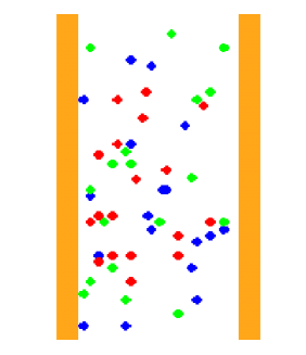
Figure 1: Collision of two hadrons. The color/grey level of the dots is an illustration of color charge of the gluons. The thickness of sheets presents the scale ${\Lambda}^{+}$ for which the color charge is defined.

In a classical field theoretical view, one can assume the sheets as an external charge configuration playing the rôle of a source for the QCD gauge field (gluon field) propagating between two hadron sheets. This is a QCD analog of a capacitor in electromagnetism. One can therefore solve the field equation and determine the field strength (gluon density) for this configuration. The main difference between this model and its electromagnetic analog is that in the latter case the charge density of the sheets is well defined. In QCD the charge depends on the energy scale, in other word depends on how close or far the observer is looking at one of the sheets (hadrons) because relating a charge to the sheet or to the swarm is not unique; closer an observer looks at the hadron, more of gluons s/he is seeing belong to the swarm in the space between sheets and less to the charge sheets [31].

This phenomenological illustration is very helpful when we want to extend hadron-hadron collision to the very high energy scales where exotic processes such as extra-dimensions can be accessible to partons [32]. For instance, if hadrons are boosted such that the physical width of the hadron sheets becomes comparable to the effective size of the bulk, at very high energy scales when slow partons leave the charge sheet, they can enter to the bulk - assuming that at these scales there is no difference (symmetry breaking) which makes the visible brane the prefered direction. According to Glass concept explained before, the partons at high energies are the parents of low energy, small $x_{B}$ partons and thus by escaping to the bulk naturally they take with them the low energy partons. This leads to a significant reduction of number of partons on the brane which must be observable. Even when gravitational force of the warping can bring back the particles to the brane, a time decoherence - equivalent to a small mass excess should be observable. Notice that this picture is Lorentz invariant. To an observer in the frame of one of the hadrons, partons of the other hadron come from very short distances and can participate in exotic processes including emission to extra-dimension.

Although it is possible to add the effect of extra-dimensions with non-flat metrics to parton evolution equation such as BFKL and CCFM, we have prefered to use the CGC model for this purpose. The reason is the consistent structure of this model which, as we will show in the next section, is manifestly Lorentz invariant. Moreover, at least formally, there is no need for many simplification assumptions in the intermediate steps which is the case for all the evolution equation formalisms.

3. Color Glass Condensate (CGC) in 4+1 Space-time with Brane Boundaries

In this section we use light-cone coordinates defined as:

$$x^{+}=x^{0}+x^{3}\quad,\quad x^{-}=x^{0}-x^{3}$$ (13)

In McLerran-Venugopalan approximation, QCD interactions are modeled by an effective $SU(3)$ gauge field $A^{B}$ of gluons. For simplicity we neglect the color index except when its explicit indication is necessary. In Light Cone (LC) gauge $A^{+}=0$. The time variation scale of color charge density on the sheet produced by the incoming hadron is much longer than the gluon swarm time scale. Therefore, it can be considered as a static charge. The classical dynamic equation of the effective gluon field is:

$$[D_{A},F^{AB}](x) = \delta^{B+}{\mathcal{W}}(x^{+},\vec{x}){\rho}_{\Lambda}^{+}(\vec{x}){\mathcal{W}}^{\dagger}(x^{+},\vec{x})$$ (14)

$${\mathcal{W}}(x^{+},\vec{x}) = T\exp\biggl{\{}ig\int_{x^{+}_{0}}^{x^{+}}d{\eta}^{+}\frac{R^{2}}{z^{2}}A^{-}({\eta}^{+},\vec{x})\biggr{\}}$$

$$D_{A} \equiv {\partial}_{;A}-igA^{a}_{A}T^{a}$$ (16)

The symbol ; means covariant derivation with respect to RS metric. Color charge $\rho$ is $+$ component of color current:

$$J^{A}(x)={\delta}^{A+}\rho(x^{-},x^{\bot},z)$$ (17)

The Wilson-line term in the right hand side of (14) guarantees the gauge invariance of this equation. The time ordering operator $T$ operates in (16) on $A^{-}\equiv A^{-}_{a}T^{a}$ and orders fields from right to left in increasing sequence of $x^{+}$.

The subscript ${\Lambda}^{+}$ of the color charge density means that it is defined at scale ${\Lambda}^{+}=x_{B}P^{+}$ where $P^{+}$ is the energy of the initial hadron. The scale ${\Lambda}^{+}$ indicates the maximum LC momentum of the parton swarm. In classical MV model it is not possible to relate models at different scales. But when quantum corrections are added, one can determine the evolution of parton density with scale ${\Lambda}^{+}$ and thereby relate the gluon distribution at $x_{B}\rightarrow 0$ to $x_{B}\rightarrow 1$ and vice versa. Physical quantities such as 2-point correlation functions at classical (tree) level are obtained from solutions of (14) integrated over all possible $\rho(x)$ with probability distribution $W_{{\Lambda}^{+}}[\rho]$.

We assume a universal coupling in the bulk and on the branes. The aim of having additional coupling on the branes in  [15] is the request for confinement of vector fields on the brane when fermions are confined. It is however easy to see that in this model fermions can’t be confined to the visible brane because this violates the gauge invariance and makes the model inconsistent.

In LC gauge equation (14) has a solution with $A^{-}=0$ in addition to the LC gauge condition $A^{+}=0$ [33]. The solution for other components is:

$$\mathcal{A}_{i}=\frac{i}{g}{\mathcal{U}}(\vec{x}){\partial}_{;i}{\mathcal{U}}^{\dagger}(\vec{x})\quad\quad i=x^{\bot},z$$ (18)

with ${\mathcal{U}}$ an element of QCD $SU(3)$ group. Unfortunately in this gauge there is no analytical way to relate ${\mathcal{U}}$ to the charge $\rho$ and to find out its explicit form. But in covariant gauge one can find an explicit solution. If we perform a gauge rotation to covariant gauge, $A^{B}$ becomes:

$$\tilde{A}^{B}={\mathcal{U}}^{\dagger}A^{B}{\mathcal{U}}+\frac{i}{g}{\mathcal{U}}^{\dagger}{\partial}^{B}_{;}{\mathcal{U}}$$ (19)

In LC gauge $A^{+}=0$ and $\tilde{A}^{+}$ has Kähler potential form:

$$\tilde{A}^{+}=\frac{i}{g}{\mathcal{U}}^{\dagger}{\partial}^{+}_{;}{\mathcal{U}}$$ (20)

and equation (14) reduces to:

$$-{\partial}_{;i}{\partial}_{;}^{i}\tilde{A^{+}} = \tilde{\rho}(\vec{x})\quad\quad i=x^{\bot},z$$ (21)

$$\tilde{\rho}(\vec{x}) \equiv {\mathcal{U}}^{\dagger}(\vec{x}){\rho}(\vec{x}){\mathcal{U}}(\vec{x})$$ (22)

$\tilde{\rho}$ is color charge density in covariant gauge. Using (21), equation (20) can be inverted and:

$${\mathcal{U}}(x^{-},x^{\bot},z)=P\exp\biggl{\{}ig\int_{x^{-}_{0}}^{x^{-}}d{\eta}^{-}\frac{R^{2}}{z^{2}}\tilde{A}^{+}({\eta}^{-},x^{\bot},z)\biggr{\}}$$ (23)

where $P$ orders $\tilde{A}^{+}\equiv\tilde{A}^{+}_{a}T^{a}$ from right to left in increasing or decreasing order of $x^{-}$ argument respectively for $x^{-}>x^{-}_{0}$ or $x^{-}<x^{-}_{0}$. We need both LC and covariant gauge formulations because in the latter gauge the solution of (14) is simpler, but the gluon distribution function has a simpler description in LC gauge.

Solution of (21) gives the propagator (Green function) in the warped 4+1 space-time. After defining the Fourier transform of $\tilde{A}^{+}$:

$$\tilde{A}^{+}(k^{\bot},z)=\int d^{2}x^{\bot}e^{ik_{\bot}x^{\bot}}\tilde{A}^{+}$$ (24)

one can expands equation (21) and obtain the equation for the propagator:

$$z^{2}{\partial}^{2}_{z}\hat{\Delta}(z,z^{\prime})+z{\partial}_{z}\hat{\Delta}(z,z^{\prime})+(k^{2}z^{2}-1)\hat{\Delta}(z,z^{\prime})=R^{2}\delta(z-z^{\prime})$$ (25)

with $k^{2}=-k_{\bot}^{2}$. General solution of (25) is:

$$\hat{\Delta}(z,z^{\prime})=C(z^{\prime})J_{1}(kz)+D(z^{\prime})N_{1}(kz)$$ (26)

where $J_{1}$ and $N_{1}$ are respectively Bessel function of first and second type. Note that the momentum of partons in the direction of the initial hadron i.e. ${\Lambda}^{+}=x_{B}P^{+}$ appears only in the scale of the model or equivalently in the color charge $\rho$. Also the dependence on $x^{-}$ is not dynamical which means that it should be fixed when boundary conditions are imposed. Integration constants $C(z^{\prime})$ and $D(z^{\prime})$ are determined by applying boundary conditions on the branes at $z=R$ and $z=R^{\prime}$. This results to following mass spectrum for KK-modes for large $n$:

$$m_{n}\approx R^{\prime-1}(\frac{3\pi}{4}\pm n\pi)$$ (27)

Therefore the coefficient $x_{n}$ in (1) for lightest modes is $\sim 2.36$. The mass of all the gluon KK-modes in this model is real. The spectrum begins from a massless zero-mode and there is a gap between zero-mode and higher modes proportional to ${\mu}^{\prime}\equiv R^{\prime-1}$ which for all macroscopic bulk is very small. In fact for large $\mu L\gtrsim 30$, even for compactification scale $\mu\sim M_{pl}$, the mass of lightest KK-modes is much smaller than CM energy of UHECR interaction in the atmosphere and when the interaction scale ${\Lambda}^{+}\gtrsim m_{n}$, KK-modes can be produced.

There is also a zero-mode with $k_{\bot}=0$ with $\hat{\Delta}(z,z^{\prime})$ satisfying:

$$z{\partial}_{z}(z{\partial}_{z}\hat{\Delta}(z,z^{\prime}))-1=\frac{R^{2}}{z^{2}}\delta(z-z^{\prime})$$ (28)

$$\hat{\Delta}(z,z^{\prime})=C_{0}(z^{\prime})z+D_{0}(z^{\prime})z^{-1}$$ (29)

After applying the boundary conditions to (29), one finds that the integration constants $C_{0}(z^{\prime})$ and $D_{0}(z^{\prime})$ are in general non-trivial and therefore the zero-mode propagates to the bulk but its wave function exponentially decreases inside the bulk. This is a well known fact [11] and contrasts with scalar field case in which the Green function of the zero-mode is $\propto\delta(z-z^{\prime})$ and consequently induces a discontinuity in the spectrum and separates zero-mode from higher KK-modes.

Propagation of gluon swarm to the bulk in MVCGC model has important implication for attempts to localize massless gauge bosons by adding an induced kinetic term on the branes. It has been shown  [22] [14] that this term increases the coupling of the zero-mode to itself and if fermions are confined to the brane, the gauge vector field becomes quasi localized. Here it is easy to see that due to $z$ dependence of $\tilde{A}^{+}$ and therefore ${\mathcal{U}}(\vec{x})$, according to (22), $\tilde{\rho}$ will depend on $z$ even when $\rho$ is confined to the brane. We will see later that because of the renormalization group equation which relates $W_{{\Lambda}^{+}}[\rho]$ the distribution of color charge density at each ${\Lambda}^{+}$ scale to other scales, $\rho$ or $\tilde{\rho}$ gradually receives a $z$ dependence, i.e. the color charge escape to the bulk even if initially - at large ${\Lambda}^{+}$ - it is concentrated on the brane. A more physical image of this process is obtained if one considers the transverse momentum ordering. At smaller $x_{B}$’s partons have larger transverse momentum because they have lost their energy by QCD radiation which at the same time increases their transverse momentum. When an extra space dimension is available, with each radiation the transverse momentum of the outing parton in the extra-dimension direction increases.

Finally gluon distribution can be calculated from the matrix elements $\langle{\mathcal{A}}_{a}^{i}{\mathcal{A}}_{b}^{j}\rangle$ after quantizing the classical solution ${\mathcal{A}}_{a}^{i}$. The definition of the gluon distribution function (structure function) in LC gauge  [34] can be extended to 4+1 space-times and results to the following expression:

$$x_{B}G(x_{B},Q^{2},z)=2J_{1}(1)P^{+}x_{B}Q^{2}\int d^{3}\vec{x}e^{iP^{+}x_{B}x^{-}}x^{\bot 2}$$

$$\int d^{3}\vec{x^{\prime}}\int_{0}^{L}dy^{\prime}e^{\mu y^{\prime}}\biggl{\langle}{\mathcal{A}}^{i}(x^{+},\vec{x^{\prime}},y^{\prime}){\mathcal{A}}_{i}(x^{+},\vec{x}-\vec{x^{\prime}},y-y^{\prime})\biggr{\rangle}$$

(30)

In this definition of gluon distribution function $Q^{2}$ is the 3-dim transverse momentum scale and $x_{B}G(x_{B},Q^{2},z)$ is the density of soft/semi-soft gluons up to $|k_{\bot}|<Q$. Due to the bounded non-flat geometry of the bulk we can not extend $|k_{\bot}|$ to the whole transverse directions. The brackets $\langle\rangle$ in (30) present both quantum mechanical expectation function and averaging over all possible configuration of color charge density $\rho(x)$. The probability functional $W_{{\Lambda}^{+}}[\rho(x)]$ for each configuration at a given scale ${\Lambda}^{+}$ can be obtain from path integral quantization of MVCGC model. It has been proved that $W_{{\Lambda}^{+}}[\rho(x)]$ evolution satisfies a renormalization group equation [35]:

$$\frac{\delta W_{\tau}[\rho]}{\delta\tau} = {\alpha}_{s}\biggl{\{}\frac{1}{2}\frac{{\delta}^{2}}{\delta{\rho}^{a}_{\tau}(x^{\bot},z)\delta{\rho}^{b}_{\tau}(x^{{}^{\prime}\bot},z^{\prime})}[W_{\tau}{\chi}^{ab}]-$$ (31)

$$\frac{\delta}{\delta{\rho}^{a}_{\tau}(x^{\bot},z)}[W_{\tau}{\sigma}^{a}]\biggr{\}}$$

where $\tau=\ln(P^{+}/{\Lambda}^{+})$. Indexes $a$ and $b$ are color indexes. Matrix elements ${\sigma}^{a}$ and ${\chi}^{ab}$ are defined as:

$${\sigma}^{a} = \langle\delta{\rho}^{a}\rangle$$ (32)

$${\chi}^{ab} = \langle\delta{\rho}^{a}\delta{\rho}^{b}\rangle$$ (33)

where $\delta{\rho}^{a}$ is the fluctuation of $\rho$ distribution from its classical value. Lowest order QCD diagrams which contribute to charge variation are discussed in  [35].

In Gaussian approximation (see (38) below) the standard deviation ${\sigma}^{2}_{{\Lambda}^{+}}\sim T_{ab}{\chi}^{ab}$ and at lowest order (BFKL approximation) [35]:

$${\sigma}^{a} \approx -g^{2}D^{+}_{y}Tr\biggl{(}T^{a}G^{i}_{0i}(x,y)\biggr{)}\biggl{|}_{x=y}$$ (34)

$${\chi}_{ab} \approx 4ig^{2}{\mathcal{F}}^{+i}_{ac}(x)\langle x|G_{0ij}|y\rangle{\mathcal{F}}^{+j}_{cb}(y)$$ (35)

$${G_{0}^{ij}}^{-1}(x) = g^{ij}{\partial}_{;B}{\partial}_{;}^{B}\quad,\quad i=\bot,z$$ (36)

where $G_{0}^{ij}$ is the propagator of free gluons. In equation (35) ${\mathcal{F}}^{+i}_{ac}$ is the gluon classical field strength of solution of (14). This approximate evaluation of $\chi$ can be used in (37) below to determine the gluon distribution up to BFKL approximation. It can be shown [32] that in this approximation the matrix elements $\langle{\mathcal{A}}_{a}^{i}{\mathcal{A}}_{b}^{j}\rangle$ have the following expression:

$$\biggl{\langle}{\mathcal{A}}_{a}^{i}(\vec{x},z){\mathcal{A}}_{bi}(\vec{x^{\prime}},z^{\prime})\biggr{\rangle}=$$

$${\delta}_{ab}\chi(\vec{x},\vec{x^{\prime}},z,z^{\prime}){\partial}_{;}^{i}{\partial^{\prime}}_{;i}\gamma(x^{\bot},x^{\prime\bot},z,z^{\prime})+\ldots$$ (37)

where:

$$\chi \equiv \frac{(zz^{\prime})^{\frac{1}{2}}}{R}\int_{-\infty}^{max(x^{-},x^{\prime-})}dx^{\prime\prime-}{\sigma}_{{\Lambda}^{+}}(x^{\prime\prime-},x^{\bot},z)$$ (38)

$${\sigma}_{{\Lambda}^{+}}(x^{\prime\prime-},x^{\prime\bot},z^{\prime})$$

and:

$$({\partial}_{;k}{\partial}_{;}^{{}^{\prime}k})^{-2}{\delta}^{3}(x^{\bot}-x^{\prime\bot},z,z^{\prime})\equiv\gamma(x^{\bot},x^{\prime\bot},z,z^{\prime})=$$

$$\frac{1}{(2\pi)^{2}}\int_{{\Lambda}_{QCD}}d^{2}k{\bot}e^{-ik_{\bot}(x^{\bot}-x^{\prime\bot})}$$

$$\int_{R}^{R^{\prime}}\frac{dz^{\prime\prime}}{R^{4}}\Delta(z^{\prime\prime},z,k^{\bot})\Delta(z^{\prime\prime},z^{\prime},k^{\bot})+\gamma(0)$$ (39)

The standard deviation of the Gaussian distribution ${\sigma}_{{\Lambda}^{+}}$ can be replaced by BFKL approximation (32).

The result of numerical calculation of the gluon distribution for the fine-tuned RS model and when the bulk scale $\mu$ is of the same order as fundamental gravity scale $M_{5}$ are respectively shown in Fig.2 and Fig.fig:rshighmu. They shows that in both cases the probability of gluon emission into the bulk is much larger than their emission into the brane. Approximations we made to obtain these distributions have a validity domain roughly the same as BFKL approximation. Nonetheless, they can be evolved to lower scales by using (31). Even without any additional calculation and just by remembering that gluons at lower scales are produced from gluons at higher scales, one can conclude that most of the softer gluons should also be emitted in the bulk. Thus, if $M_{5}\lesssim 10^{15}eV$, one had to observe a much lower flux for the high energy wing of UHECRs. In fact not only it does not seem to be the case, the observed flux is much higher than classical expectations and either a top-down model of a decaying heavy dark matter or extremely exotic astronomical sources are needed to explain their flux.

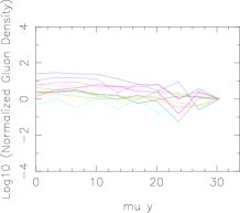
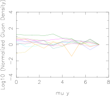
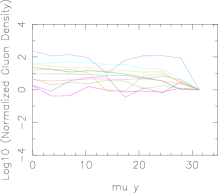
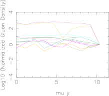
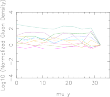
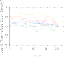
Figure 2: Gluon distribution in the bulk normalized to the amplitude of the distribution on the visible brane at $z=R^{\prime}$ for Randall-Sundrum models for $2\times 10^{8}eV\leqslant|k_{\bot}|\leqslant 1.26\times 10^{10}eV$. Curves are rainbow color/grey coded. From bottom to top $M_{5}=10^{13}eV,10^{14}eV$ and $10^{15}eV$, with $\mu$ obtained from fine-tuned RS model (5) i.e. $\mu=10^{-17}eV,10^{-14}eV$ and $10^{-11}eV$ respectively. For left plots $\log(R^{\prime}/R)=\log(M_{pl}/M_{5})$, i.e. the same as (4). In right panel a smaller $R^{\prime}/R$ is used to see the effect of a smaller bulk with same fundamental gravitation and compactification scale. Our tests show that apparent vibration of the distribution is mainly due to low resolution of our numerical calculation.

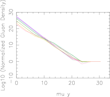
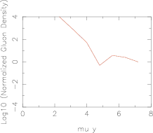
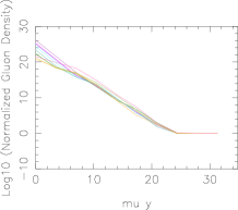
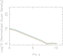
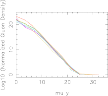
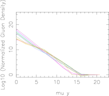
Figure 3: The same as Fig.2 but with $\mu=M_{5}$. Other details are the same as Fig.2. In the top right plot the difference between curves for different $k^{\bot}$ is much smaller than the resolution of this figure and they are overlapped.

4. Classical Propagation of Relativistic Particles in the Bulk

Now that we have shown that high energy particles in a hadron-hadron collision penetrate to the bulk, we would like to use the classical propagation of these particles in the bulk to constrain other brane model. The reason is that although the MVCGC formalism or other evolution models such as CCFM can be extended to any brane model, for more complex metrics the calculation becomes very difficult. For a simple order of magnitude estimation of parameter space, a time of flight estimation can be adequate. The general form of the metric of a 4+1 dimensional space-time with curved bulk is:

$$ds^{2}=n^{2}(t,y)dt^{2}-a^{2}(t,y)\delta_{ij}dx^{i}dx^{j}-b^{2}(t,y)dy^{2}.$$ (40)

In a gauge where $b(t,y)=1$, after solving Einstein equations and applying boundary conditions on the branes, one obtains the following solutions for $a(t,y)$ and $n(t,y)$:

$$a^{2}(t,y)={\mathcal{A}}(t)\cosh(\mu y)+{\mathcal{B}}(t)\sinh(\mu y)+{\mathcal{C}}(t)$$ (41)

$$\dot{a}^{2}(t,y) = n^{2}(t,y)a_{0}^{2}(t)=$$

$$\frac{\biggl{(}\dot{\mathcal{A}}(t)\cosh(\mu y)+\dot{\mathcal{B}}(t)\sinh(\mu y)+\dot{\mathcal{C}}(t)\biggr{)}^{2}}{4a^{2}(t,y)}$$

$${\mathcal{A}}(t) = {a_{0}}^{2}(t)-{\mathcal{C}(t)}$$ (43)

$${\mathcal{B}}(t) = -{\rho}^{\prime}_{b_{0}}{a_{0}}^{2}(t)$$ (44)

$${\mathcal{C}}(t) = -\frac{2{{\dot{a}}_{0}}^{2}(t)}{{\mu}^{2}}$$ (45)

$$\mu \equiv \sqrt{\frac{2{\hat{\kappa}}^{2}}{3}|{\rho}_{B}|}$$ (46)

$$n(t,y) = \frac{\dot{a}(t,y)}{\dot{a}_{0}(t)}$$ (47)

For any density $\rho$, ${\rho}^{\prime}\equiv\rho/{\Lambda}_{RS}$, ${\Lambda}_{RS}\equiv 3\mu/{\hat{\kappa}}^{2}$. The densities ${\rho}^{\prime}_{b_{0}}$ and ${\rho}_{B}$ are respectively effective total energy density of the brane at $y=0$ and the bulk. We consider only AdS bulk models with ${\rho}_{B}<0$. The constant ${\hat{\kappa}}^{2}=8\pi/M_{5}^{3}$ is the gravitational coupling in the 5-dim. space-time. The model dependent details such as how ${\rho}^{\prime}_{b_{0}}$ and ${\rho}_{B}$ are related to the field contents in the bulk and on the brane and how they evolve are irrelevant for us as long as we assume a quasi-static model. The solution (41) is valid both for one brane and multi-brane models. The only difference between them is in the application of Israel junction conditions [36] [37]. After changing the variable $y$ to $z=e^{\mu y}$ and using (47):

$$\dot{a}^{2}(t,z) = -\frac{{\mu}^{2}{\mathcal{C}}(t)}{2z}{\mathcal{D}}(t,z)$$ (48)

$${\mathcal{D}} \equiv \frac{1}{2}\biggl{[}(1-{\rho}^{\prime}_{b_{0}}-\frac{{\mathcal{C}}(t)}{a^{2}_{0}})z^{2}+\frac{2{\mathcal{C}}(t)}{a^{2}_{0}}z+$$ (49)

$$(1+{\rho}^{\prime}_{b_{0}}-\frac{{\mathcal{C}}(t)}{a^{2}_{0}})\biggr{]}$$

$$\frac{dz}{dt} = \mu\sqrt{{\mathcal{D}}(z-\frac{\epsilon}{{\theta}^{2}}{\mathcal{D}})}$$ (50)

$\theta$ is an integration constant. If an ejected particle to the bulk comes back to the brane, its velocity in the bulk must approach to zero at its turning point before the particle arrives to the bulk horizon (if it is present). The roots of (50) correspond to these turning points and determine the propagation time in the bulk. The typical propagation time we are interested in is much shorter than the age of the Universe and therefore ${\mathcal{A}},{\mathcal{B}},{\mathcal{C}}$ and $\dot{\mathcal{A}},\dot{\mathcal{B}},\dot{\mathcal{C}}$ during propagation are roughly constant. The right hand side of (50) depends only on $z$ and is easily integrable:

$${\Delta}t_{propag}\equiv 2(t_{stop}-t_{0})=\int_{z_{0}}^{z_{stop}}\frac{2dz}{\mu\sqrt{{\mathcal{D}}(z-\frac{\epsilon}{{\theta}^{2}}{\mathcal{D}})}}$$ (51)

In (51), $t_{0}$ is the initial time of propagation in the extra-dimension and $t_{stop}$ is the time when the particle’s velocity changes its direction, i.e. when $dz/dt=0$. The integral in (51) is related to the elliptical integrals of the first type ${\mathcal{F}}(\omega,\nu)$ where $\omega$ and $\nu$ are analytical functions of the denominator roots in (51) and $z_{0}$. Note that $z_{stop}$ corresponds to the closest root to $z_{0}$.

Using this simple model, we determine the propagation time of relativistic particles in the bulk for some of the most popular brane models. This time delay must be smaller than the time resolution of air-shower detectors as no time decoherence - delay between arrival of most energetic particles - has been observed.

Fig.4 shows ${\Delta}t_{propag}$ as a function of $\mu L$ and $M_{5}$ for massive relativistic particles. With present air shower detectors time resolution of order $10^{-6}sec$, only when $M_{5}\gtrsim 10^{18}eV$, the model is compatible with the observed time coherence of the UHE showers. For fine-tuned RS model $\mu\approx G/{\hat{\kappa}}^{2}$  [2] i.e. ${\mu}=GM_{5}^{3}\sim 10^{-3}eV$ for $M_{5}\sim 10^{18}eV$  [2]. Due to smallness of $\mu$ and consequently lightness of KK-modes for SM particles even this model with large $M_{5}$ has already been ruled out [14] unless a conserved quantum number prevents the production of KK-modes [38]. For massless particles:

$$z(t)-z_{0}=\mu(t-t_{0})^{2}$$ (52)

In (52), $z(t)$ is monotonically increasing and there is no stopping point. With our approximations there is no horizon in the bulk because $a(t,y)$ is roughly constant. Therefore, equation(52) means that massless particles simply continue their path to the hidden brane and their faith depends on what happen to them there. At very high CM energy of UHECR interactions if charged particles can escape to the bulk photons are also dragged to the bulk and never come back. This is very similar to the conclusion of more precise and completely independent formulation of the previous section and shows that the logic behind them are consistent.

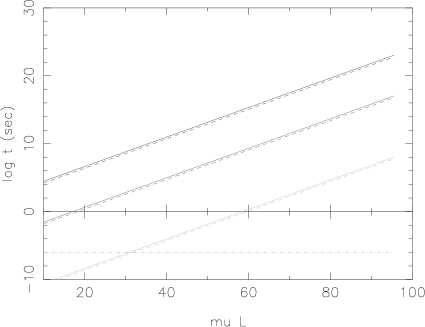
Figure 4: Propagation time for relativistic particles with Lorentz factor $u^{0}_{L}(t_{0})/N=10^{3}$ (full line) and $u^{0}_{L}(t_{0})/N=1.2$ (dash line) in RS model. From top to buttom curves correspond to $M_{5}=10^{13}eV$, $M_{5}=10^{15}eV$ and $M_{5}=10^{18}eV$ (or $\mu\sim 10^{-17}eV$, $\mu\sim 10^{-11}eV$ and $\mu\sim 10^{-2}eV$ for fine-tuned model) respectively. The horizontal line shows the time coherence precision of present Air Shower detectors.

Next we consider the case of a general 2-brane model. Numerical solution of constrained 2-brane models in  [36] [37] shows that for $\mu L\gtrsim 5$ the tension on both branes can be positive and very close to ${\Lambda}_{RS}$. We use constraints on the Cosmological Constant and hierarchy to find ${\rho}^{\prime}_{0}$ and ${\rho}^{\prime}_{L}={\rho}^{\prime}_{b}$, the branes tension. We redefine them as ${\rho}^{\prime}_{0}=1+\Delta{\rho}^{\prime}_{0}$ and ${\rho}^{\prime}_{L}=1+\Delta{\rho}^{\prime}_{L}$. To solve hierarchy problem the following constraint must be fulfilled:

$$\frac{M^{2}_{5}}{M^{2}_{pl}}\sim N^{2}\equiv\frac{n^{2}_{L}}{n^{2}_{0}}=\frac{{\rho}^{\prime}_{{\Lambda}_{0}}(1-\cosh(\mu L))+\sinh(\mu L)}{{\rho}^{\prime}_{{\Lambda}_{L}}(1-\cosh(\mu L))+\sinh(\mu L)}\ll 1$$ (53)

This leads to:

$$\Delta{\rho}^{\prime}_{0} = \frac{N^{2}\biggl{(}1-e^{-\mu L}+\Delta{\rho}^{\prime}_{L}(1-\cosh(\mu L)\biggr{)}}{1-\cosh(\mu L)}-$$ (54)

$$\frac{1-e^{-\mu L}}{1-\cosh(\mu L)}$$

For a very small $N^{2}$ and $\Delta{\rho}^{\prime}_{L}\lesssim 1$, the first term in (54) is ${\mathcal{O}}(N^{2})$ and:

$$\Delta{\rho}^{\prime}_{0}\approx-\frac{1-e^{-\mu L}}{1-\cosh(\mu L)}\approx-\frac{1}{1-\cosh(\mu L)}\approx 2e^{-\mu L}$$ (55)

Using $\dot{a}^{2}_{L}/{a}^{2}_{L}=H^{2}$ where $H$ is the Hubble Constant on the visible brane [37]:

$$\Delta{\rho}^{\prime}_{L}=\frac{1}{2N^{2}\sinh(\mu L)}$$

$$\biggl{[}(1-\cosh(\mu L))\frac{2H^{2}}{{\mu}^{2}}+e^{-\mu L}-1\pm$$

$$\biggl{(}\biggl{(}(1-\cosh(\mu L))\frac{2H^{2}}{{\mu}^{2}}+e^{-\mu L}-1\biggr{)}^{2}+$$

$$N^{2}\sinh(\mu L)(\frac{2H^{2}}{{\mu}^{2}}+2e^{-\mu L})\biggr{)}^{\frac{1}{2}}\biggr{]}$$ (56)

In (56) the solution with plus sign gives $\Delta{\rho}^{\prime}_{L}\approx-2$ which deviates from our first assumption $|\Delta{\rho}^{\prime}_{L}|<1$ and leads to a negative tension on the visible brane like static RS model. The solution with negative sign is $\Delta{\rho}^{\prime}_{L}\approx 2e^{-\mu L}$ and both branes have positive tension close to ${\Lambda}_{RS}$.

Using these values for the tensions in (41) to (47), we can find the time delay for this class of brane models:

$$\Delta t_{propag} = \frac{4}{\mu(8|\Delta{\rho}^{\prime}_{0}+{\mathcal{C}}^{\prime}|)^{\frac{1}{4}}}{\mathcal{F}}(\alpha,Q)$$ (57)

$$\alpha = 2\arctan\sqrt{\frac{q(z_{-}-z_{0})}{p(z_{0}-z_{+})}}$$ (58)

$$Q = \frac{1}{2}\biggl{(}2+\frac{2}{pq}$$

$$\biggl{[}\frac{{\mathcal{C}}^{\prime}({\mathcal{C}}^{\prime}-{\theta}^{2})+4(2+\Delta{\rho}^{\prime}_{0}+{\mathcal{C}}^{\prime})(\Delta{\rho}^{\prime}_{0}+{\mathcal{C}}^{\prime})}{(\Delta{\rho}^{\prime}_{0}+{\mathcal{C}}^{\prime})^{2}}\biggr{]}\biggr{)}^{\frac{1}{2}}$$

$$p^{2} \equiv \biggl{(}\frac{{\mathcal{C}}^{\prime}}{\Delta{\rho}^{\prime}_{0}+{\mathcal{C}}^{\prime}}-z_{-}\biggr{)}^{2}+r^{2}$$ (60)

$$q^{2} \equiv \biggl{(}\frac{{\mathcal{C}}^{\prime}}{\Delta{\rho}^{\prime}_{0}+{\mathcal{C}}^{\prime}}-z_{+}\biggr{)}^{2}+r^{2}$$ (61)

$$r^{2} \equiv -\biggl{(}\frac{{\mathcal{C}}^{\prime}}{\Delta{\rho}^{\prime}_{0}+{\mathcal{C}}^{\prime}}\biggr{)}^{2}-\biggl{(}\frac{2+\Delta{\rho}^{\prime}_{0}+{\mathcal{C}}^{\prime}}{\Delta{\rho}^{\prime}_{0}+{\mathcal{C}}^{\prime}}\biggr{)}$$ (62)

$$-{\mathcal{C}}^{\prime} = \Delta{\rho}^{\prime}_{0}+\frac{2}{z_{0}}(N^{2}+\Delta{\rho}^{\prime}_{0})$$ (63)

In (58), $z_{0}=e^{\mu L}$ and, $z_{\pm}$ are the roots of velocity amplitude. The result of the numerical calculation of the time delay for these models is shown in Fig.5. We conclude that for these models the time delay can not constraint the value of $M_{5}$, but put constraint on $\mu L$, roughly speaking the warp factor. This means that by adjusting the warping, it is always possible to make the time delay too short to be observable at present air-shower detectors. Nevertheless, in these models $\mu$ is not arbitrary and depends on $\mu L$. On the other hand, in many radion models for stabilizing the bulk, $\mu$ is related to the mass of radion and its value must be in the range requested by the models for stabilization. Therefore comparing the results presented here permits to investigate which type of stabilization and particle physics behind them can satisfy all the constraints. Test of more models can be found in  [23]

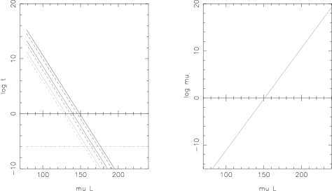
Figure 5: Left: Propagation time for relativistic particles in 2-brane model. Description of the curves is the same as Fig.4. Right: Parameter $\mu(eV)$ as a function of $\mu L$. It is roughly independent of $M_{5}$.

5. conclusion

In this proceedings we tried to show that physics in future colliders and air-shower detectors is crowded by low energy effects and great efforts must be dedicated to extract information about new physics hidden deep inside collision events.

We investigated the effect of the escape of partons to a warped bulk. We showed that it can significantly reduces the total cross-section and multiplicity - number of final state particles emitted into the brane. To arrive to this conclusion we needed to use an evolution equation to related the low energy observables to high energy parton (gluon) distribution in hadron-hadron collisions. We used the recently developed phenomenological model Color Glass Condensate and extended it to 4+1 warped space-times with brane boundaries and static Randall-Sundrum metrics.

Inspired by the observation that relativistic particles can be emitted to the bulk, we have also used a simple classical model of propagation of relativistic particles in bulk for more general type of brane models and obtained constraints both for the fundamental scale of gravity and for parameters of the brane models.

Acknowledgement

I would like to thank the organizers of the Cosmion-2004 conference and very specially Dr. K. Belotsky and Pr. M. Khlopov.

References

- [1] N. Arkani-Hamed, S. Dimopoulos and G. Dvali, Phys. Lett. B 429, 263 (1998) hep-ph/9807344; I. Antoniadis, et al., Phys. Lett. B 436, 257 (1998) hep-ph/9804398.
- [2] L. Randall and R. Sundrum, Phys. Rev. Lett. 83, 3370 (1999) hep-ph/9905221, L. Randall and R. Sundrum, Phys. Rev. Lett. 83, 4690 (1999) hep-ph/9906064.
- [3] V.A. Rubakov and M.E. Shaposhinkov, Phys. Lett. B 125, 139 (1983), K. Akama, Lect. Notes Phys. 176, 267 (1982).
- [4] I. Antoniadis, Phys. Lett. B 246, 377 (1990).
- [5] P. Horava and E. Witten, Nucl. Phys. B 460, 506 (1996) hep-th/9510209, Nucl. Phys. B 475, 94 (1996) hep-th/9603142.
- [6] W.D. Goldberger and M.B. Wise, Phys. Rev. Lett. 83, 4922 (1999) hep-ph/9907447.
- [7] P. Binétruy, J.M. Cline and C. Grojean, Phys. Lett. B 489, 403 (2000) hep-th/0007029.
- [8] Sh. Kobayashi, K. Koyama and J. Soda, Phys. Lett. B 501, 157 (2001) hep-th/0009160.
- [9] R. Gregory, V.A. Rubakov and S.M. Sibiryakov, Phys. Rev. Lett. 84, 5928 (2000) hep-th/0002072, W. Mück, K.S. Viswanathan and I.V. Volovich, Phys. Rev. D 62, 105019 (2000) hep-th/0002132, R. Gregory, V.A. Rubakov and S.M. Sibiryakov, Class.Quant.Grav. 17, 4437 (2000) hep-th/0003109.
- [10] S.L. Dubovsky, V.A. Rubakov, P.G. Tinyakov, Phys. Rev. D 62, 105011 (2000) hep-th/0006046, J. High Ener. Phys. 0008, 041 (2000) hep-ph/0007179.
- [11] B. Bajc and G. Gabadadze, Phys. Lett. B 474, 282 (2000) hep-th/9912232.
- [12] S.L. Dubovsky, J. High Ener. Phys. 0201, 012 (2002) hep-th/0103205.
- [13] S.L. Dubovsky, V.A. Rubakov, Int. J. Mod. Phys. A 16, 4331 (2001) hep-th/0105243.
- [14] H. Davoudiasl, J.L. Hewett and T.G. Rizzo, Phys. Lett. B 473, 43 (2000) hep-ph/9911262, H. Davoudiasl, J.L. Hewett and T.G. Rizzo, Phys. Rev. D 68, 045002 (2003) hep-ph/0212279, H. Davoudiasl, J.L. Hewett and T.G. Rizzo, J. High Ener. Phys. 0308, 034 (2003) hep-ph/0305086.
- [15] G.Dvali, G. Gabadadze and M. Porrati, Phys. Lett. B 484, 112 (2000) hep-th/0002190, G. Dvali, G. Gabadadze and M. Porrati,Phys. Lett. B 484, 129 (2000) hep-th/0003054.
- [16] S.L. Dubovsky, V.A. Rubakov and P.G. Tinyakov, Phys. Rev. Lett. 85, 3769 (2000) hep-ph/0006046, J. High Ener. Phys. 0008, 041 (2000) hep-ph/0007179.
- [17] M. Carena, T.M.P. Tait, and C.E.M. Wagner, Acta Phys.Polon. B 33, 2355 (2002) hep-ph/0207056.
- [18] S. Dimopoulos and G.F. Giudice, Phys. Lett. B 379, 105 (1996), J.C. Long, H.W. Chan and J.C. Price, Nucl. Phys. B 539, 23 (1999) hep-ph/9805217.
- [19] N. Arkani-Hamed, S. Dimopoulos and G. Dvali, PLB 429, 263 (1998) hep-ph/9807344, M. Fairbairn and L.M. Griffiths, J. High Ener. Phys. 0202, 024 (2002) hep-ph/0111435.
- [20] G.F. Giudice, R. Rattazzi, J.D. and Wells, Nucl. Phys. B 544, 3 (1999) hep-ph/9811291, L.J. Hall and D. Smith, Phys. Rev. D 60, 085008 (1999) hep-ph/9904267.
- [21] H. Davoudiasl, J.L. Hewett and T.G. Rizzo Phys. Rev. D 63, 075004 (2001) hep-ph/0006041.
- [22] G. Dvali, G. Gabadadze and M. Shifman, Phys. Lett. B 497, 271 (2001) hep-th/0010071.
- [23] H. Ziaeepour, “Testing Brane World Models with Ultra High Energy Cosmic Rays”, hep-ph/0203165.
- [24] S.B. Giddings, E. Katz and L. Randall, J. High Ener. Phys. 0003, 023 (2000) hep-th/0002091.
- [25] A. Kotikov and L. Lipotov, Nucl. Phys. B 661, 19 (2003) hep-ph/0208220.
- [26] V. Gribov and L. Lipatov, Sov.J. Nucl. Phys. 15, 438 (1972) and 675, L. Lipotov, Sov.J. Nucl. Phys. 20, 94 (1975), G. Altarelli and G. Parisi, Nucl. Phys. B 126, 298 (1977), Y. Dokshitser, Sov.J. Phys. JETP 46, 641 (1977).
- [27] E. Kuraev, L. Lipatov, V. Fadin Sov.J. Phys. JETP 44, 443 (1976),Sov.J. Phys. JETP 45, 199 (1977), Y. Balitskii, L. Lipatov, Sov.J. Nucl. Phys. 28, 822 (1978).
- [28] B. Anderson, et al.(The small x Collaboration) “Small Phenomenology Summary and Status”, hep-ph/0204115, hep-ph/0312333.
- [29] S. Catani, F. Fiorani and G. Marchesini Phys. Lett. B 234, 339 (1990) and Nucl. Phys. B 336, 18 (1990), G. Marchesini Nucl. Phys. B 445, 49 (1995).
- [30] L. McLerran and R. Venugopalan, Phys. Rev. D 49, 2233 (1994), L. McLerran and R. Venugopalan, Phys. Rev. D 49, 3352 (1994), L. McLerran and R. Venugopalan, Phys. Rev. D 50, 2225 (1994).
- [31] L. McLerran, “What is the Evidence for Color Glass Condensate”, hep-ph/0402137.
- [32] H. Ziaeepour, “Color Glass Condensate in Brane Models”, hep-ph/0407046.
- [33] J. Jalalian-Marian, et al., Phys. Rev. D 55, 5414 (1997) hep-ph/9606337.
- [34] A.H. Mueller, “Small- Physics, High Parton Densities and Parton Saturation in QCD”, hep-ph/9911289.
- [35] E. Iancu, A. Leonidov, and L. McLerran, Nucl. Phys. A 692, 583 (2001) hep-ph/0011241, E. Ferreiro, E. Iancu, A. Leonidov, and L. McLerran, Nucl. Phys. A 703, 489 (2002) hep-ph/0109115.
- [36] P. Kanti, K.A. Olive and M. Pospelov, Phys. Rev. D 62, 126004 (2000) hep-ph/0005146.
- [37] H. Ziaeepour, “Two-Brane Models and BBN”, hep-ph/0010180.
- [38] T. Appelquist, H.C. Cheng and B.A. Dobrescu, Phys. Rev. D 64, 035002 (2001) hep-ph/0012100, G. Servant and T.M.P. Tait, Nucl. Phys. B 650, 391 (2003) hep-ph/0206071.