Data for Polarization in Charmless $B\to\phi K^{*}$: A Signal for New Physics?

Abstract

The recent observations of sizable transverse fractions of $\overline{B}\to\phi\overline{K}^{*}$ may hint for the existence of new physics. We analyze all possible new-physics four-quark operators and find that two classes of new-physics operators could offer resolutions to the $\overline{B}\to\phi\overline{K}^{*}$ polarization anomaly. The operators in the first class have structures $(1-\gamma_{5})\otimes(1-\gamma_{5}),\sigma(1-\gamma_{5})\otimes\sigma(1-\gamma_{5})$, and in the second class $(1+\gamma_{5})\otimes(1+\gamma_{5}),\sigma(1+\gamma_{5})\otimes\sigma(1+\gamma_{5})$. For each class, the new physics effects can be lumped into a single parameter. Two possible experimental results of polarization phases, $\arg(A_{\perp})-\arg(A_{\parallel})\approx\pi$ or $0$, originating from the phase ambiguity in data, could be separately accounted for by our two new-physics scenarios: the first (second) scenario with the first (second) class new-physics operators. The consistency between the data and our new physics analysis, suggests a small new-physics weak phase, together with a large(r) strong phase. We obtain sizable transverse fractions $\Lambda_{\parallel\parallel}+\Lambda_{\perp\perp}\approx\Lambda_{00}$, in accordance with the observations. We find $\Lambda_{\parallel\parallel}\simeq 0.8\Lambda_{\perp\perp}$ in the first scenario but $\Lambda_{\parallel\parallel}\gtrsim\Lambda_{\perp\perp}$ in the second scenario. We discuss the impact of the new-physics weak phase on observations.

I Introduction

The studies for two-body charmless $B$ decays have raised a lot of interests among the particle physics community. Recently the BABAR and BELLE collaborations have presented important results for the $B$ meson decaying to a pair of light vector mesons (with $V=\phi,\rho$, or $K^{*}$) Aubert:2003mm ; Aubert:2003xc ; Aubert:2004xc ; Zhang:2003up ; Chen:2003jf ; Abe:2004ku . This immediately surges a considerable amount of theoretical attentions to study nonperturbative features or to look for the possibility of having new physics (NP) in order to explain several discrepancies between the data and the Standard Model (SM) based calculations Kagan ; Hnli ; Colangelo:2004rd ; Cheng:2004ru ; Ladisa:2004bp ; Dariescu:2003tx ; Hou:2004vj .

From the existing SM calculations for the charmless $\overline{B}\rightarrow VV$ modes, it is known that the amplitude, $\overline{H}_{00}$ ($\sim{\cal O}(1)$), with two vector mesons in the longitudinal polarization state is much greater than those in transverse polarization states, since the latter are found to be $\overline{H}_{--}\sim{\cal O}(1/m_{b}),\overline{H}_{++}\sim{\cal O}(1/m_{b}^{2})$ (or $\overline{A}_{\|}\simeq\overline{A}_{\perp}\sim{\cal O}(1/m_{b})$ in the transversity basis) CY . For the $B$ meson decays, the relation for different helicity amplitudes is modified as $H_{00}:H_{++}:H_{--}\sim{\cal O}(1):{\cal O}(1/m_{b}):{\cal O}(1/m_{b}^{2})$. Nevertheless, recently BABAR Aubert:2003mm ; Aubert:2004xc first observed sizable transverse fractions in the $\overline{B}\to\phi\overline{K}^{*}$ decays, where the transverse polarization amplitudes are comparable to the longitudinal one. This result was confirmed later by BELLE Chen:2003jf ; Abe:2004ku . In other words, in terms of helicity amplitudes the data show that $|\overline{H}_{++}\pm\overline{H}_{--}|^{2}\approx|\overline{H}_{00}|^{2}$ (or $2|\overline{A}_{\|}|^{2}\approx 2|\overline{A}_{\perp}|^{2}\approx|\overline{A}_{0}|^{2}$ in the transversity basis). Such an anomaly in transverse fractions is rather unexpected within the SM framework. Efforts have already been made for finding a possible explanation in the SM or NP scenario. In the SM, according to Kagan Kagan , the nonfactorizable contributions due to the annihilation could give rise to the following logarithmic divergent contributions to the helicity amplitudes: ${\overline{H}}_{00},{\overline{H}}_{--}\sim{\cal O}[(1/m_{b}^{2})\ln^{2}(m_{b}/\Lambda_{h})]$, ${\overline{H}}_{++}\sim{\cal O}[(1/m_{b}^{4})\ln^{2}(m_{b}/\Lambda_{h})]$, where $\Lambda_{h}$ is the typical hadronic scale. This in turn may enhance the transverse amplitudes required to explain the anomaly. However, in the perturbative QCD (PQCD) framework, Li and Mishima Hnli have shown that the annihilations are still not sufficient to enhance transverse fractions. Another possibility for explaining the polarization anomaly advocated by Colangelo et al. Colangelo:2004rd is the existence of large charming penguin and final state interaction (FSI) effects. However they got $|A_{0}|^{2}(B\to\rho K^{*})<|A_{0}|^{2}(B\to\phi K^{*})$, in contrast to the observations Aubert:2003mm ; Aubert:2003xc ; Aubert:2004xc ; Zhang:2003up ; Chen:2003jf ; Abe:2004ku , where the normalization $\sum_{i}|A_{i}|^{2}=1$ is adopted. With the similar FSI scenario, Cheng et al. Cheng:2004ru obtained $|A_{0}|^{2}:|A_{\|}|^{2}:|A_{\perp}|^{2}=0.43:0.54:0.03$, which is also in contrast to the recent data Aubert:2004xc ; Abe:2004ku . Now the question is: Is it possible to explain this anomaly by the NP? If yes, what types of NP operators one should consider? Some NP related models have been proposed Dariescu:2003tx , where the so-called right-handed currents $\bar{s}\gamma_{\mu}(1+\gamma_{5})b\ \bar{s}\gamma^{\mu}(1\pm\gamma_{5})s$ were emphasized Kagan . If the right-handed currents contribute constructively to $\overline{A}_{\perp}$ but destructively to $\overline{A}_{0,\|}$, then one may have larger $|\overline{A}_{\perp}/\overline{A}_{0}|^{2}$ to account for the data. However the resulting $|\overline{A}_{\|}|^{2}\ll|\overline{A}_{\perp}|^{2}$ Kagan will be in contrast to the recent observations Aubert:2004xc ; Abe:2004ku . See also the detailed discussions in Sec. II.

In the present study, we consider general cases of 4-quark operators. Taking into account all possible color and Lorentz structures, totally there are 20 NP four-quark operators which do not appear in the SM effective Hamiltonian (see Eqs. (LABEL:eq:vectorop) and (31)). After analyzing the helicity properties of quarks arising from various four-quark operators, we find that only two classes of four-quark operators are relevant in resolving the transverse anomaly. The first class is made of operators with structures $\sigma(1-\gamma_{5})\otimes\sigma(1-\gamma_{5})$ and $(1-\gamma_{5})\otimes(1-\gamma_{5})$, which contribute to different helicity amplitudes as ${\overline{H}_{00}}:{\overline{H}_{--}}:{\overline{H}_{++}}\sim{\cal O}(1/m_{b}):{\cal O}(1/m_{b}^{2}):{\cal O}(1)$. The second class consists of operators with structures $\sigma(1+\gamma_{5})\otimes\sigma(1+\gamma_{5})$ and $(1+\gamma_{5})\otimes(1+\gamma_{5})$, from which the resulting amplitudes read as ${\overline{H}_{00}}:{\overline{H}_{++}}:{\overline{H}_{--}}\sim{\cal O}(1/m_{b}):{\cal O}(1/m_{b}^{2}):{\cal O}(1)$. Moreover, the above (pseudo-)scalar operators can be written in terms of their companions, the (axial-)tensor operators, by Fierz transformation. Finally, there is only one effective coefficient relevant for each class. We find that these two classes can separately satisfy the two possible solutions for polarization phase data, which is due to the phase ambiguity in the measurement, and the anomaly for large transverse fractions can thus be resolved. The tensor operator effects were first noticed by Kagan Kagan (see Sec. II for further discussions).

The organization of the paper is as follows. In Sec. II, we first introduce the SM results for the polarization amplitudes in the ${\overline{B}^{0}}\to\phi{\overline{K}}^{*0}$ decay within the QCD factorization (QCDF) framework. After that we give a detailed discussion about how the NP can play a crucial role in resolving the large transverse polarization anomaly as observed by BELLE and BABAR. The reason for choosing the two classes of operators with structures (i) $\sigma(1-\gamma_{5})\otimes\sigma(1-\gamma_{5}),(1-\gamma_{5})\otimes(1-\gamma_{5})$ and (ii) $\sigma(1+\gamma_{5})\otimes\sigma(1+\gamma_{5}),(1+\gamma_{5})\otimes(1+\gamma_{5})$ is explained and the relevant calculations arising from these operators are performed. We discuss the possibility for the existence of right-handed currents $\bar{s}\gamma_{\mu}(1+\gamma_{5})b\ \bar{s}\gamma^{\mu}(1\pm\gamma_{5})s$ which was emphasized in Kagan . From the point of view of helicity conservation in the strong interactions, we discuss various contributions originating from the chromomagnetic dipole operator, charming penguin mechanism, and annihilations. Some observables relevant in our numerical analysis are defined in this section. In Sec. III, we summarize input parameters e.g. Kobayashi-Maskawa (KM) elements, form factors, meson decay constants, required for our study. Sec. IV is fully devoted to the numerical analysis. We discuss in detail two scenarios, which are separately consistent with the two possible polarization phase solutions in data due to the phase ambiguity. We obtain the best fit values for the NP parameters which can resolve the polarization anomaly. Numerical results for observables are collected in this section. Finally, in Sec. V, we summarize our results and make our conclusion.

II Framework

II.1 The Standard Model results in the QCD factorization approach

The best starting point for describing nonleptonic charmless $B$ decays is to write down first the effective Hamiltonian describing the processes. The processes of our concern are the $\overline{B}\to\phi\overline{K}^{*}$ decays which are penguin dominated. In the SM, the relevant effective weak Hamiltonian ${\cal H}_{\rm eff}$ for the above $\Delta B=1$ transitions is

$${\cal H}_{\rm eff}=\frac{G_{F}}{\sqrt{2}}\left[V_{ub}V_{us}^{*}\left(c_{1}O_{1}^{u}+c_{2}O_{2}^{u}\right)+V_{cb}V_{cs}^{*}\left(c_{1}O_{1}^{c}+c_{2}O_{2}^{c}\right)-V_{tb}V_{ts}^{*}\left(\sum_{i=3}^{10}c_{i}O_{i}\right)+c_{g}O_{g}\right]+{\rm H.c.}.$$ (1)

Here $c_{i}$’s are the Wilson coefficients and the 4-quarks current-current, penguin and chromomagnetic dipole operators are defined by

• current-current operators:

  $$O_{1}^{u} = ({\overline{u}}b)_{V-A}({\overline{s}}u)_{V-A}~{}~{}~{}~{}O_{2}^{u}=({\overline{u}_{\alpha}}b_{\beta})_{V-A}({\overline{s}}_{\beta}u_{\alpha})_{V-A},$$

  $$O_{1}^{c} = ({\overline{c}}b)_{V-A}({\overline{s}}c)_{V-A}~{}~{}~{}~{}O_{2}^{c}=({\overline{c}_{\alpha}}b_{\beta})_{V-A}({\overline{s}}_{\beta}c_{\alpha})_{V-A},$$ (2)

• QCD-penguin operators:

  $$O_{3} = ({\overline{s}}b)_{V-A}\sum_{q}({\overline{q}}q)_{V-A},~{}~{}~{}~{}O_{4}=({\overline{s}_{\alpha}}b_{\beta})_{V-A}\sum_{q}({\overline{q}}_{\beta}q_{\alpha})_{V-A},$$

  $$O_{5} = ({\overline{s}}b)_{V-A}\sum_{q}({\overline{q}}q)_{V+A},~{}~{}~{}~{}O_{6}=({\overline{s}_{\alpha}}b_{\beta})_{V-A}\sum_{q}({\overline{q}}_{\beta}q_{\alpha})_{V+A},$$ (3)

• electroweak-penguin operators:

  $$O_{7} = \frac{3}{2}({\overline{s}}b)_{V-A}\sum_{q}e_{q}({\overline{q}}q)_{V+A},~{}~{}~{}~{}O_{8}=\frac{3}{2}({\overline{s}_{\alpha}}b_{\beta})_{V-A}\sum_{q}e_{q}({\overline{q}}_{\beta}q_{\alpha})_{V+A},$$

  $$O_{9} = \frac{3}{2}({\overline{s}}b)_{V-A}\sum_{q}e_{q}({\overline{q}}q)_{V-A},~{}~{}~{}~{}O_{10}=\frac{3}{2}({\overline{s}_{\alpha}}b_{\beta})_{V-A}\sum_{q}e_{q}({\overline{q}}_{\beta}q_{\alpha})_{V-A},$$ (4)

• chromomagnetic dipole operator:

  $$O_{8g}=\frac{g_{s}}{8\pi^{2}}m_{b}{\overline{s}}\sigma^{\mu\nu}(1+\gamma_{5})T^{a}bG^{a}_{\mu\nu},$$ (5)

where $\alpha,\beta$ are the $SU(3)$ color indices, $V\pm A$ correspond to $\gamma^{\mu}(1\pm\gamma^{5})$, the Wilson coefficients $c_{i}$’s are evaluated at the scale $\mu$, $e$ and $g$ are respectively QED and QCD coupling constants and $T^{a}$’s are $SU(3)$ color matrices. For the penguin operators, $O_{3},\dots,O_{10}$, the sum over $q$ runs over different quark flavors, active at $\mu\simeq m_{b}$, i.e. $q~{}\epsilon\{u,d,s,c,b\}$.

In the present work, we will embark on the study of $\overline{B}\to\phi\overline{K}^{*}$ decays in the approach of the QCDF. The ${\overline{B}}^{0}\rightarrow\phi{\overline{K}^{*0}}$ decay amplitude with the $\phi$ meson being factorized CY reads

$${\overline{A}}({\overline{B}}^{0}\rightarrow\phi{\overline{K}^{*0}})_{SM}=\frac{G_{F}}{\sqrt{2}}\left(-V_{tb}V_{ts}^{*}\right)\left[a_{3}+a_{4}+a_{5}-\frac{1}{2}(a_{7}+a_{9}+a_{10})\right]X^{({\overline{B}}^{0}{\overline{K}^{*0}},\phi)},$$ (6)

which is penguin dominated. The annihilation contribution which is power suppressed is neglected here CY . The $B^{0}\rightarrow\phi K^{*0}$ decay amplitude can be obtained by considering CP transformation. As far as the charged $B$-meson decay is concerned, the dominant contribution also comes from the penguin operators, while the contribution due to $O_{1},O_{2}$ is color and KM suppressed. In the scenario, where $\phi$ is factorized, the decay amplitudes for $B^{0},{\overline{B}^{0}},B^{+},B^{-}$ are almost the same. The factor $X^{({\overline{B}}^{0}{\overline{K}^{*0}},\phi)}$ in Eq. (6) is equal to

$$X^{({\overline{B}}^{0}{\overline{K}^{*0}},\phi)} = \langle\phi(q,\epsilon_{1})|({\overline{s}}s)_{V-A}|0\rangle\langle{\overline{K}^{*0}}(p^{\prime},\epsilon_{2})|({\overline{s}}b)_{V-A}|{\overline{B}}^{0}(p)\rangle,$$ (7)

$$= if_{\phi}m_{\phi}\left[\frac{-2i}{m_{B}+m_{K^{*}}}\epsilon_{\mu\nu\alpha\beta}\epsilon_{1}^{*\mu}\epsilon_{2}^{*\nu}p^{\alpha}p^{\prime\beta}V(q^{2})\right]$$

$$-if_{\phi}m_{\phi}\left[(m_{B}+m_{K^{*}})\epsilon_{1}^{*}\cdot\epsilon_{2}^{*}A_{1}(q^{2})-(\epsilon_{1}^{*}\cdot p)(\epsilon_{2}^{*}\cdot p)\frac{2A_{2}(q^{2})}{m_{B}+m_{K^{*}}}\right],$$

where the decay constants and form factors are defined by

$$\langle\phi(q,\epsilon_{1})|V^{\mu}|0\rangle = f_{\phi}m_{\phi}\epsilon_{1}^{\mu*},$$

$$\langle{\overline{K}^{*0}}(p^{\prime},\epsilon_{2})|V^{\mu}|{\overline{B}}^{0}(p)\rangle = \frac{2}{m_{B}+m_{K^{*}}}\epsilon^{\mu\nu\alpha\beta}\epsilon_{2\nu}^{*}p_{\alpha}p_{\beta}^{\prime}V(q^{2}),$$

$$\langle{\overline{K}^{*0}}(p^{\prime},\epsilon_{2})|A^{\mu}|{\overline{B}}^{0}(p)\rangle = i\left[(m_{B}+m_{K^{*}})\epsilon_{2}^{*\mu}A_{1}(q^{2})-(\epsilon_{2}^{*}\cdot p)(p+p^{\prime})^{\mu}\frac{A_{2}(q^{2})}{m_{B}+m_{K^{*}}}\right]$$ (8)

$$-2im_{K^{*}}\frac{\epsilon_{2}^{*}\cdot p}{q^{2}}q^{\mu}\left[A_{3}(q^{2})-A_{0}(q^{2})\right],$$

with $m_{B}$ and $m_{K^{*}}$ being the masses of ${\overline{B}^{0}}$ and ${\overline{K}^{*0}}$ mesons, respectively, $q=p-p^{\prime}$, $A_{3}(0)=A_{0}(0)$, and

$$A_{3}(q^{2})=\frac{m_{B}+m_{K^{*}}}{2m_{K^{*}}}A_{1}(q^{2})-\frac{m_{B}-m_{K^{*}}}{2m_{K^{*}}}A_{2}(q^{2}).$$ (9)

It is straightforward to write down the decay width,

$$\Gamma(\overline{B}^{0}\rightarrow\phi{\overline{K}^{*0}})=\frac{p_{c}}{8\pi m_{B}^{2}}\left(|{\overline{H}_{00}}|^{2}+|{\overline{H}_{++}}|^{2}+|{\overline{H}_{--}}|^{2}\right),$$ (10)

where $p_{c}$ is the center mass momentum of the $\phi$ or $\overline{K}^{*0}$ meson in the $\overline{B}$ rest frame. ${\overline{H}_{00}}$, ${\overline{H}_{++}}$, ${\overline{H}_{--}}$ are the decay amplitudes in the helicity basis and in QCDF , they are given by

$${\overline{H}_{00}}=\frac{G_{F}}{\sqrt{2}}(V_{tb}V_{ts}^{*})a^{0}_{SM}(if_{\phi}m_{\phi})(m_{B}+m_{K^{*}})\left[aA_{1}(m_{\phi}^{2})-bA_{2}(m_{\phi}^{2})\right],$$

$${\overline{H}_{\pm\pm}}=-\frac{G_{F}}{\sqrt{2}}(V_{tb}V_{ts}^{*})a^{\pm}_{SM}(if_{\phi}m_{\phi})\left[(m_{B}+m_{K^{*}})A_{1}(m_{\phi}^{2})\mp\frac{2m_{B}p_{c}}{m_{B}+m_{K^{*}}}V(m_{\phi}^{2})\right],$$ (11)

with the constants $a=(m_{B}^{2}-m_{\phi}^{2}-m_{K^{*}}^{2})/(2m_{\phi}m_{K^{*}})$, $b=(2m_{B}^{2}p_{c}^{2})/[m_{\phi}m_{K^{*}}(m_{B}+m_{K^{*}})^{2}]$. Here $a^{h}_{SM}=a^{h}_{3}+a^{h}_{4}+a^{h}_{5}-\frac{1}{2}(a^{h}_{7}+a^{h}_{9}+a^{h}_{10})$. The superscript $h$ in $a_{i}^{h}$’s denotes the polarization of $\phi$ and $\overline{K}^{*0}$ mesons; $h=0$ is for the helicity 00 state and $h=\pm$ for helicity $\pm\pm$ states. Note that the weak phase effect is tiny in $a^{h}_{SM}$ and is thus neglected in the study. Such helicity dependent effective coefficients $a^{h}_{SM}$ do arise in the QCDF, however in the naive factorization (NF), they turns out to be same, i.e. $a^{0}_{SM}=a^{+}_{SM}=a^{-}_{SM}=a_{SM}$. In the NF, one can rewrite the above amplitudes in the transversity basis as

$${\overline{A}}_{0}^{SM} = \frac{G_{F}}{\sqrt{2}}(V_{tb}V_{ts}^{*})a_{SM}(if_{\phi}m_{\phi})(m_{B}+m_{K^{*}})\left[aA_{1}(m_{\phi}^{2})-bA_{2}(m_{\phi}^{2})\right],$$

$${\overline{A}}_{\|}^{SM} = -\frac{G_{F}}{\sqrt{2}}(V_{tb}V_{ts}^{*})a_{SM}(i{\sqrt{2}}f_{\phi}m_{\phi})(m_{B}+m_{K^{*}})A_{1}(m_{\phi}^{2}),$$

$${\overline{A}}_{\perp}^{SM} = -\frac{G_{F}}{\sqrt{2}}(V_{tb}V_{ts}^{*})a_{SM}({i\sqrt{2}}f_{\phi}m_{\phi})\frac{2p_{c}m_{B}}{(m_{B}+m_{K^{*}})}V(m_{\phi}^{2}).$$ (12)

In the QCDF, $a_{i}^{h}$’s are given by

$$a_{1}^{h} = c_{1}+{c_{2}\over N_{c}}+{\alpha_{s}\over 4\pi}\,{C_{F}\over N_{c}}c_{2}\,(F^{h}+f_{II}^{h}),$$

$$a_{2}^{h} = c_{2}+{c_{1}\over N_{c}}+{\alpha_{s}\over 4\pi}\,{C_{F}\over N_{c}}c_{1}\,(F^{h}+f_{II}^{h}),$$

$$a_{3}^{h} = c_{3}+{c_{4}\over N_{c}}+{\alpha_{s}\over 4\pi}\,{C_{F}\over N_{c}}c_{4}\,(F^{h}+f_{II}^{h}),$$

$$a_{4}^{h} = c_{4}+{c_{3}\over N_{c}}+{\alpha_{s}\over 4\pi}\,{C_{F}\over N_{c}}\Bigg{\{}c_{3}\big{[}(F^{h}+f_{II}^{h})+G^{h}(s_{s})+G^{h}(s_{b})\big{]}-c_{1}\left({\lambda_{u}\over\lambda_{t}}G^{h}(s_{u})+{\lambda_{c}\over\lambda_{t}}G^{h}(s_{c})\right)$$

$$+(c_{4}+c_{6})\sum_{i=u}^{b}\biggl{(}G^{h}(s_{i})-{2\over 3}\biggr{)}+{3\over 2}(c_{8}+c_{10})\sum_{i=u}^{b}e_{i}\biggl{(}G^{h}(s_{i})-{2\over 3}\biggr{)}$$

$$+{3\over 2}c_{9}\big{[}e_{q}G^{h}(s_{q})-{1\over 3}G^{h}(s_{b})\big{]}+c_{g}G^{h}_{g}\Bigg{\}},$$

$$a_{5}^{h} = c_{5}+{c_{6}\over N_{c}}-{\alpha_{s}\over 4\pi}\,{C_{F}\over N_{c}}c_{6}(\tilde{F}^{h}+f_{II}^{h}+12),$$

$$a_{6}^{h} = c_{6}+{c_{5}\over N_{c}},$$

$$a_{7}^{h} = c_{7}+{c_{8}\over N_{c}}-{\alpha_{s}\over 4\pi}\,{C_{F}\over N_{c}}c_{8}(\tilde{F}^{h}+f_{II}^{h}+12)-{\alpha\over 9\pi}\,N_{c}C^{h}_{e},$$

$$a_{8}^{h} = c_{8}+{c_{7}\over N_{c}},$$

$$a_{9}^{h} = c_{9}+{c_{10}\over N_{c}}+{\alpha_{s}\over 4\pi}\,{C_{F}\over N_{c}}c_{10}\,(F^{h}+f_{II}^{h})-{\alpha\over 9\pi}\,N_{c}C^{h}_{e},$$

$$a_{10}^{h} = c_{10}+{c_{9}\over N_{c}}+{\alpha_{s}\over 4\pi}\,{C_{F}\over N_{c}}c_{9}\,(F^{h}+f_{II}^{h})-{\alpha\over 9\pi}\,C^{h}_{e},$$ (13)

where $C_{F}=(N_{c}^{2}-1)/(2N_{c})$, $s_{i}=m_{i}^{2}/m_{b}^{2}$, $\lambda_{q}=V_{qb}V^{*}_{qq^{\prime}}$, and $q^{\prime}=d,s$. Note that we have given the expressions for $a_{1}^{h}$, $a_{2}^{h}$, which may be relevant for charged $B$ decays, arising due to $O_{1}$ and $O_{2}$ in Eq. (1). There are QCD and electroweak penguin-type diagrams induced by the 4-quark operators $O_{i}$ for $i=1,3,4,6,8,9,10$. These corrections are described by the penguin-loop function $G^{h}(s)$ given by

$$G^{0}(s) = {2\over 3}-{4\over 3}\ln{\mu\over m_{b}}+4\int^{1}_{0}du\,\Phi^{\phi}_{\|}(u)\int^{1}_{0}dx\,x(1-x)\ln[s-\bar{u}x(1-x)],$$

$$G^{\pm}(s) = {2\over 3}-{2\over 3}\ln{\mu\over m_{b}}$$ (14)

$$+2\int^{1}_{0}du\,\Bigg{(}g^{\phi(v)}_{\perp}(u)\pm{1\over 4}{dg_{\perp}^{\phi(a)}(u)\over du}\Bigg{)}\int^{1}_{0}dx\,x(1-x)\ln[s-\bar{u}x(1-x)]\,.$$

In Eq. (II.1) we have also included the leading electroweak penguin-type diagrams induced by the operators $O_{1}$ and $O_{2}$,

$$C_{e}^{h} = \left({\lambda_{u}\over\lambda_{t}}G^{h}(s_{u})+{\lambda_{c}\over\lambda_{t}}G^{h}(s_{c})\right)\left(c_{2}+{c_{1}\over N_{c}}\right).$$ (15)

The dipole operator $O_{8g}$ will give a tree-level contribution proportional to

$$G^{0}_{g}=-2\int^{1}_{0}du\,{\Phi^{\phi}_{\|}(u)\over 1-u}\,,$$

$$G^{\pm}_{g}=\int^{1}_{0}{du\over\bar{u}}\,\Bigg{[}\int_{0}^{u}\,\Big{(}\Phi_{\|}^{\phi}(v)-g^{\phi(v)}_{\perp}(v)\Big{)}dv-\bar{u}g_{\perp}^{\phi(v)}(u)\mp{{\bar{u}}\over 4}{dg_{\perp}^{\phi(a)}(u)\over du}+{g_{\perp}^{\phi(a)}(u)\over 4}\Bigg{]}\,,$$ (16)

In Eq. (II.1), the vertex correction is given by

$$F^{h}=-12\ln{\mu\over m_{b}}-18+f_{I}^{h},$$ (17)

where we have used the naïve dimensional regularization (NDR) scheme Buras:1990fn ,

$$\gamma_{\mu}\gamma_{\nu}\gamma_{\lambda}(1-\gamma_{5})\otimes\gamma^{\mu}\gamma^{\nu}\gamma^{\lambda}(1-\gamma_{5})=4(4-\varepsilon)\gamma_{\mu}(1-\gamma_{5})\otimes\gamma^{\mu}(1-\gamma_{5}),$$ (18)

$$\gamma_{\mu}\gamma_{\nu}\gamma_{\lambda}(1-\gamma_{5})\otimes\gamma^{\lambda}(1-\gamma_{5})\gamma^{\nu}\gamma^{\mu}=4(1-2\varepsilon)\gamma_{\mu}(1-\gamma_{5})\otimes\gamma^{\mu}(1-\gamma_{5}),$$ (19)

$$\gamma_{\mu}\gamma_{\nu}\gamma_{\lambda}(1-\gamma_{5})\otimes\gamma^{\mu}\gamma^{\nu}\gamma^{\lambda}(1+\gamma_{5})=4(1+\varepsilon)\gamma_{\mu}(1-\gamma_{5})\otimes\gamma^{\mu}(1+\gamma_{5}),$$ (20)

$$\gamma_{\mu}\gamma_{\nu}\gamma_{\lambda}(1-\gamma_{5})\otimes\gamma^{\lambda}(1+\gamma_{5})\gamma^{\nu}\gamma^{\mu}=4(4-4\varepsilon)\gamma_{\mu}(1-\gamma_{5})\otimes\gamma^{\mu}(1+\gamma_{5}),$$ (21)

with $D=4-2\varepsilon$, and have adopted the $\overline{\rm MS}$ substraction. An explicit calculation for $f_{I}^{h}$, arising from vertex corrections, yields

$$f_{I}^{0} = \int^{1}_{0}dx\,\Phi_{\|}^{\phi}(x)\left(3{1-2x\over 1-x}\ln x-3i\pi\right),$$

$$f_{I}^{\pm} = \int^{1}_{0}dx\,\Bigg{(}g_{\perp}^{\phi(v)}(x)\pm{1\over 4}\frac{dg_{\perp}^{\phi(a)}(x)}{dx}\Bigg{)}\left(3{1-2x\over 1-x}\ln x-3i\pi\right).$$ (22)

The hard kernel $f_{II}^{h}$ for hard spectator interactions, arising from the hard spectator interactions with a hard gluon exchange between the emitted vector meson and the spectator quark of the $B$ meson, have the expressions:

$$f_{II}^{0} = {4\pi^{2}\over N_{c}}\,{2f_{B}f_{K^{*}}m_{K^{*}}\over h_{0}}\int^{1}_{0}d\rho\,{\Phi^{B}_{1}(\rho)\over\bar{\rho}}\int^{1}_{0}d\eta\,{\Phi^{K^{*}}_{\|}(\eta)\over\bar{\eta}}\int^{1}_{0}d\xi\,{\Phi^{\phi}_{\|}(\xi)\over\xi},$$

$$f_{II}^{\pm} = -{4\pi^{2}\over N_{c}}\,{f_{B}f^{T}_{K^{*}}\over m_{B}h_{\pm}}(1\mp 1)\int^{1}_{0}d\rho\,{\Phi^{B}_{1}(\rho)\over\bar{\rho}}\int^{1}_{0}d\eta\,{\Phi^{K^{*}}_{\perp}(\eta)\over\bar{\eta}^{2}}\int^{1}_{0}d\xi\,$$ (23)

$$\ \ \ \times\Bigg{[}2\Bigg{(}g_{\perp}^{\phi(v)}(\xi)-{1\over 4}\frac{dg_{\perp}^{\phi(a)}(\xi)}{d\xi}\Bigg{)}+\Bigg{(}\frac{1}{\xi}-\frac{1}{\bar{\xi}}\Bigg{)}\int_{0}^{\xi}dv(\Phi_{\parallel}^{\phi}(v)-g_{\perp}^{\phi(v)}(v))\Bigg{]}$$

$$+{4\pi^{2}\over N_{c}}\,{2f_{B}f_{K^{*}}m_{K^{*}}\over m_{B}^{2}h_{\pm}}\int^{1}_{0}d\rho\,{\Phi^{B}_{1}(\rho)\over\bar{\rho}}\int^{1}_{0}d\eta\,\Bigg{(}g^{K^{*}(v)}_{\perp}(\eta)\pm{1\over 4}{dg^{K^{*}(a)}_{\perp}(\eta)\over d\eta}\Bigg{)}\int^{1}_{0}d\xi$$

$$\ \ \ \times\Bigg{\{}\frac{\bar{\eta}+\bar{\xi}}{\bar{\eta}^{2}\bar{\xi}}\Bigg{(}g_{\perp}^{\phi(v)}(\xi)\pm{1\over 4}{dg_{\perp}^{\phi(a)}(\xi)\over d\xi}\Bigg{)}+\frac{1}{\bar{\eta}^{2}\xi}\int_{0}^{\xi}dv(\Phi_{\parallel}^{\phi}(v)-g_{\perp}^{\phi(v)}(v))\Bigg{\}},$$

where

$$h_{0} = (m_{B}^{2}-m_{K^{*}}^{2}-m_{\phi}^{2})(m_{B}+m_{K^{*}})A^{B{K^{*}}}_{1}(m_{\phi}^{2})-{4m_{B}^{2}p_{c}^{2}\over m_{B}+m_{K^{*}}}\,A^{B{K^{*}}}_{2}(m_{\phi}^{2}),$$

$$h_{\pm} = (m_{B}+m_{K^{*}})A^{B{K^{*}}}_{1}(m_{\phi}^{2})\mp{2m_{B}p_{c}\over m_{B}+m_{K^{*}}}\,V^{B{K^{*}}}(m_{\phi}^{2}).$$ (24)

Note that $\tilde{F}^{h}$ can be obtained from $F^{h}$ in Eq. (17) with the replacement of $g_{\perp}^{\prime\,\phi(a)}\to-g_{\perp}^{\prime\,\phi(a)}$. We will introduce a cutoff of order $\Lambda_{\rm QCD}/m_{b}$ to regulate the infrared divergence in $f_{II}$. Note also that we have corrected  the QCDF results in Ref. CY which were done by Cheng and one of us (K.C.Y.). The key point for the calculation is that one needs to consider correctly the projection operator in the momentum space, as discussed in Appendix A, which may explain the difference with Ref. Li:2003he  . In the calculation, we take the asymptotic light-cone distribution amplitudes (LCDAs) for the light vector mesons, and a Gaussian form for the $B$ meson wave function. CY . We now make a SM estimate for various helicity amplitudes from a power counting point of view. For $\overline{B}^{0}\to\phi\overline{K}^{*0}$, the helicity amplitude ${\overline{H}_{00}}$ arising from the $(V-A)\otimes(V-A)$ operators is ${\cal O}(1)$, since each of $\phi$ and $\overline{K}^{*0}$ mesons, with the quark and antiquark being left and right-handed helicities, respectively, requires no helicity flip. For ${\overline{H}_{--}}$, the helicity flip for the $\bar{s}$ quark in the $\phi$ meson is required, resulting in $m_{\phi}/m_{b}$ suppression for the amplitude. Finally in ${\overline{H}_{++}}$ two helicity flips for $s$ quarks are required, one in $\phi$ meson and the other in the $\overline{B}^{0}\to{\overline{K}^{*0}}$ form factor transition, which cause a suppression by $(m_{\phi}/m_{b})(\bar{\Lambda}/m_{b})$, where $\bar{\Lambda}=m_{B}-m_{b}$. In a nutshell, the three helicity amplitudes in the SM can be approximated as ${\overline{H}_{00}}:{\overline{H}_{--}}:{\overline{H}_{++}}\sim{\cal O}(1):{\cal O}(1/m_{b}):{\cal O}(1/m_{b}^{2})$. One should note that for the CP-conjugated ${B^{0}}\rightarrow\phi K^{*0}$, the above result is modified to be $H_{00}:H_{++}:H_{--}\sim{\cal O}(1):{\cal O}(1/m_{b}):{\cal O}(1/m_{b}^{2})$. The results extended to various possible NP operators together with the SM operators will be shown later in Table 1 and also illustrated in Fig. 1.

II.2 New physics: hints from the BABAR and BELLE observations

The large transverse $\overline{B}\to\phi\overline{K}^{*}$ fractions as have been observed by BELLE and BABAR Aubert:2003xc ; Chen:2003jf ; Aubert:2004xc ; Abe:2004ku , may hint a departure from the SM expectation for the longitudinal one. Within the SM, the QCDF calculation CY yields

$$1-R_{0}={\cal O}(1/m_{b}^{2})=R_{T}\,,$$ (25)

where $R_{0}=|\overline{A}_{0}|^{2}/|\overline{A}_{tot}|^{2}$ and $R_{T}=R_{\|}+R_{\perp}=(|\overline{A}_{\|}|^{2}+|\overline{A}_{\perp}|^{2})/|\overline{A}_{tot}|^{2}$. The observation of large $R_{T}$, as large as $50\%$, may be possible to be accounted for in the SM, but here we are considering the new physics alternatively . In the transversity basis the recent experiments Aubert:2004xc ; Abe:2004ku have shown that

$$|A_{0}|^{2}(=|\overline{H}_{00}|^{2})\approx|\overline{A}_{T}|^{2}(=|\overline{A}_{\|}|^{2}+|\overline{A}_{\perp}|^{2})\,,$$ (26)

where $\overline{A}_{\|}=(\overline{H}_{++}+\overline{H}_{--})/{\sqrt{2}}$ and $\overline{A}_{\perp}=-(\overline{H}_{++}-\overline{H}_{--})/{\sqrt{2}}$. One may need NP to explain such a large $R_{T}$ ($\approx R_{0}$). A set of NP operators contributing to the different helicity amplitudes like

$$\overline{H}_{00}:\overline{H}_{--}:\overline{H}_{++} \sim {\cal O}(1/m_{b}):{\cal O}(1):{\cal O}(1/m_{b}^{2})\,,$$ (27)

or

$${\overline{H}_{00}}:{\overline{H}_{--}}:{\overline{H}_{++}} \sim {\cal O}(1/m_{b}):{\cal O}(1/m_{b}^{2}):{\cal O}(1)\,,$$ (28)

could resolve such polarization anomaly. Note that $\overline{H}_{--}$ (in the former case) and $\overline{H}_{++}$ (in the latter case) are of ${\cal O}(1)$, while $\overline{H}_{00}$ is always of ${\cal O}(1/m_{b})$, in contrast to the SM expectation. The detailed reason will be seen below.

II.2.1 New physics operators

Now Eqs. (27) and (28) can serve as guideline in selecting NP operators. To begin with, consider the following effective Hamiltonian ${\cal H}^{\rm NP}$:

$${\cal H}^{\rm NP}=\frac{G_{F}}{\sqrt{2}}\sum_{i=11}^{30}\left[c_{i}(\mu)O_{i}(\mu)\right]+H.c.\,,$$ (29)

which may be generated from some NP sources and contains the following general NP four-operators:

• four-quark operators with vector and axial-vector structures:

  $$O_{11} = {\overline{s}}\gamma^{\mu}(1+\gamma^{5})b~{}{\overline{s}}\gamma_{\mu}(1+\gamma^{5})s\,,\ \ \ \ O_{12}={\overline{s}_{\alpha}}\gamma^{\mu}(1+\gamma^{5})b_{\beta}~{}{\overline{s}}_{\beta}\gamma_{\mu}(1+\gamma^{5})s_{\alpha}\,,$$

  $$O_{13} = {\overline{s}}\gamma^{\mu}(1+\gamma^{5})b~{}{\overline{s}}\gamma_{\mu}(1-\gamma^{5})s\,,\ \ \ \ O_{14}={\overline{s}_{\alpha}}\gamma^{\mu}(1+\gamma^{5})b_{\beta}~{}{\overline{s}}_{\beta}\gamma_{\mu}(1-\gamma^{5})s_{\alpha}\,,$$

• four-quark operators with scalar and pseudo-scalar structures:

  $$O_{15} = {\overline{s}}(1+\gamma^{5})b~{}{\overline{s}}(1+\gamma^{5})s\,,\ \ \ \ O_{16}={\overline{s}_{\alpha}}(1+\gamma^{5})b_{\beta}~{}{\overline{s}}_{\beta}(1+\gamma^{5})s_{\alpha}\,,$$

  $$O_{17} = {\overline{s}}(1-\gamma^{5})b~{}{\overline{s}}(1-\gamma^{5})s\,,\ \ \ \ O_{18}={\overline{s}_{\alpha}}(1-\gamma^{5})b_{\beta}s~{}{\overline{s}}_{\beta}(1-\gamma^{5})s_{\alpha}\,,$$

  $$O_{19} = {\overline{s}}(1+\gamma^{5})b~{}{\overline{s}}(1-\gamma^{5})s\,,\ \ \ \ O_{20}={\overline{s}_{\alpha}}(1+\gamma^{5})b_{\beta}~{}{\overline{s}}_{\beta}(1-\gamma^{5})s_{\alpha}\,,$$

  $$O_{21} = {\overline{s}}(1-\gamma^{5})b~{}{\overline{s}}(1+\gamma^{5})s\,,\ \ \ \ O_{22}={\overline{s}_{\alpha}}(1-\gamma^{5})b_{\beta}~{}{\overline{s}}_{\beta}(1+\gamma^{5})s_{\alpha}\,,$$ (31)

• four-quark operators with tensor and axial-tensor structures:

  $$O_{23} = {\overline{s}}\sigma^{\mu\nu}(1+\gamma^{5})b~{}{\overline{s}}\sigma_{\mu\nu}(1+\gamma^{5})s\,,\ \ \ \ O_{24}={\overline{s}_{\alpha}}\sigma^{\mu\nu}(1+\gamma^{5})b_{\beta}~{}{\overline{s}}_{\beta}\sigma_{\mu\nu}(1+\gamma^{5})s_{\alpha}\,,$$

  $$O_{25} = {\overline{s}}\sigma^{\mu\nu}(1-\gamma^{5})b~{}{\overline{s}}\sigma_{\mu\nu}(1-\gamma^{5})s\,,\ \ \ \ O_{26}={\overline{s}_{\alpha}}\sigma^{\mu\nu}(1-\gamma^{5})b_{\beta}~{}{\overline{s}}_{\beta}\sigma_{\mu\nu}(1-\gamma^{5})s_{\alpha}\,,$$

  $$O_{27} = {\overline{s}}\sigma^{\mu\nu}(1+\gamma^{5})b~{}{\overline{s}}\sigma_{\mu\nu}(1-\gamma^{5})s\,,\ \ \ \ O_{28}={\overline{s}_{\alpha}}\sigma^{\mu\nu}(1+\gamma^{5})b_{\beta}~{}{\overline{s}}_{\beta}\sigma_{\mu\nu}(1-\gamma^{5})s_{\alpha}\,,$$

  $$O_{29} = {\overline{s}}\sigma^{\mu\nu}(1-\gamma^{5})b~{}{\overline{s}}\sigma_{\mu\nu}(1+\gamma^{5})s\,,\ \ \ \ O_{30}={\overline{s}_{\alpha}}\sigma^{\mu\nu}(1-\gamma^{5})b_{\beta}~{}{\overline{s}}_{\beta}\sigma_{\mu\nu}(1+\gamma^{5})s_{\alpha}\,.$$

Here $c_{i}$ with $i=11,\dots,30$ are the Wilson coefficients of the corresponding NP operators and $\mu$ the renormalization scale, chosen to be $m_{b}$ here. Now we give an estimation of several types of NP operators, contributing to various ${\overline{B}^{0}}\to\phi\overline{K}^{*}$ helicity amplitudes. In Fig. 1, we draw the diagrams in the $\overline{B}$ rest frame, where $q_{1},q_{3}$ are the $s$ quarks, and $\bar{q}_{2}$ is the $\bar{s}$ quark. ($q_{1},\bar{q}_{2}$) and ($q_{3},\bar{q}_{4}$) form $\phi$ and $\overline{K}^{*}$, respectively. $q_{4}$ is the spectator light quark which has not any preferable direction. $q_{1},\bar{q}_{2},q_{3}$ are originated from the following operators: $\bar{q}_{3}\Gamma_{1}b\ \bar{q}_{1}\Gamma_{2}q_{2}$ for $O_{3-6},O_{11-14},O_{23-30}$ or $\bar{q}_{1}\Gamma_{1}b\ \bar{q}_{3}\Gamma_{2}q_{2}$ for $O_{15-22}$. If the helicity for $q_{1}$ or $\bar{q}_{2}$ is flipped, then the amplitude is suppressed by a factor of $m_{\phi}/m_{b}$. On the other hand, if the helicity of $q_{3}$ is further flipped, the amplitude will be suppressed by $(m_{\phi}/m_{b})(\bar{\Lambda}/m_{b})$, with $\bar{\Lambda}=m_{B}-m_{b}$. The results are summarized in Table 1.

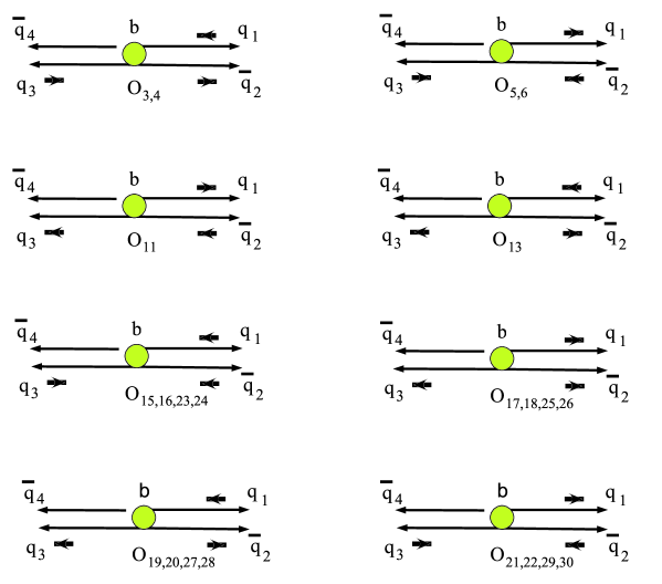
Figure 1: The main helicity directions of quarks and antiquarks arising from various four-quark operators during the $\overline{B}$ decay, where the solid circle denotes the $b$ quark, $q_{1},q_{3}$ are the $s$ quarks, and $\bar{q}_{2}$ is the $\bar{s}$ quark. ($q_{1},\bar{q}_{2}$) and ($q_{3},\bar{q}_{4}$) form $\phi$ and $\overline{K}^{*}$, respectively. $\bar{q}_{4}$ is the spectator light quark which has no preferable direction. The short arrows denote the helicities of quarks and antiquarks. See the text for the detailed discussions.

Table 1: Possible NP operators and their candidacy in satisfying the anomaly resolution criteria. We have adopted the convention $\Gamma_{1}\otimes\Gamma_{2}\equiv{\overline{s}}\Gamma_{1}b\ {\overline{s}}\Gamma_{2}s$.

Model	Operators	$\overline{H}_{00}$	$\overline{H}_{--}$	$\overline{H}_{++}$	Choice
SM	$\gamma^{\mu}(1-\gamma_{5})\otimes\gamma_{\mu}(1\mp\gamma_{5})$	${\cal O}(1)$	${\cal O}(1/m_{b})$	${\cal O}(1/m_{b}^{2})$
NP	$\gamma^{\mu}(1+\gamma_{5})\otimes\gamma_{\mu}(1+\gamma_{5})$	${\cal O}(1)$	${\cal O}(1/m_{b}^{2})$	${\cal O}(1/m_{b})$	N
NP	$\gamma^{\mu}(1+\gamma_{5})\otimes\gamma_{\mu}(1-\gamma_{5})$	${\cal O}(1)$	${\cal O}(1/m_{b}^{2})$	${\cal O}(1/m_{b})$	N
NP	$(1+\gamma_{5})\otimes(1+\gamma_{5})$	${\cal O}(1/m_{b})$	${\cal O}(1)$	${\cal O}(1/m_{b}^{2})$	Y
NP	$(1-\gamma_{5})\otimes(1-\gamma_{5})$	${\cal O}(1/m_{b})$	${\cal O}(1/m_{b}^{2})$	${\cal O}(1)$	Y
NP	$(1+\gamma_{5})\otimes(1-\gamma_{5})$	${\cal O}(1)$	${\cal O}(1/m_{b}^{2})$	${\cal O}(1/m_{b})$	N
NP	$(1-\gamma_{5})\otimes(1+\gamma_{5})$	${\cal O}(1)$	${\cal O}(1/m_{b})$	${\cal O}(1/m_{b}^{2})$	N
NP	$\sigma^{\mu\nu}(1+\gamma_{5})\otimes\sigma_{\mu\nu}(1+\gamma_{5})$	${\cal O}(1/m_{b})$	${\cal O}(1)$	${\cal O}(1/m_{b}^{2})$	Y
NP	$\sigma^{\mu\nu}(1-\gamma_{5})\otimes\sigma_{\mu\nu}(1-\gamma_{5})$	${\cal O}(1/m_{b})$	${\cal O}(1/m_{b}^{2})$	${\cal O}(1)$	Y
NP	$\sigma^{\mu\nu}(1+\gamma_{5})\otimes\sigma_{\mu\nu}(1-\gamma_{5})$	${\cal O}(1)$	${\cal O}(1/m_{b}^{2})$	${\cal O}(1/m_{b})$	N
NP	$\sigma^{\mu\nu}(1-\gamma_{5})\otimes\sigma_{\mu\nu}(1+\gamma_{5})$	${\cal O}(1)$	${\cal O}(1/m_{b})$	${\cal O}(1/m_{b}^{2})$	N

From the Table 1, we see that both (pseudo-)scalar operators $O_{15-18}$ and (axial-)tensor operators $O_{23-26}$ satisfy the anomaly resolution criteria as given by Eqs. (27) and (28), while the rest are not. However, through the Fierz transformation, it can be shown that $O_{15,16}$ and $O_{17,18}$ operators can be expressed as a linear combination of $O_{23,24}$ and $O_{25,26}$ operators, respectively, i.e.,

$$O_{15} = \frac{1}{12}O_{23}-\frac{1}{6}O_{24},$$

$$O_{16} = \frac{1}{12}O_{24}-\frac{1}{6}O_{23},$$

$$O_{17} = \frac{1}{12}O_{25}-\frac{1}{6}O_{26},$$

$$O_{18} = \frac{1}{12}O_{26}-\frac{1}{6}O_{25}.$$ (33)

Before we continue the study, five remarks are in order. (i) The $\bar{s}\sigma^{\mu\nu}(1+\gamma_{5})b\ \bar{s}\sigma_{\mu\nu}(1+\gamma_{5})s$ operator, which could maintain $|\overline{A}_{\perp}|^{2}\approx|\overline{A}_{\|}|^{2}$, was first mentioned by Kagan Kagan  . (ii) We do not consider NP of left-handed currents, $\bar{s}\gamma_{\mu}(1-\gamma_{5})b\ \bar{s}\gamma^{\mu}(1\mp\gamma_{5})s$, which give corrections to SM Wilson coefficients, $c_{1-10}$, since they have no help for understanding large polarized amplitudes and are strongly constrained by other $B\to PP,VP$ observations hfag . (iii) $O_{11-14}$ are the so-called right-handed currents, emphasized recently by Kagan Kagan . These operators give corrections to amplitudes as

$$\overline{A}_{0,\|} \propto (-V_{tb}V_{ts}^{*})a_{SM}-(a_{11}+a_{12}+a_{13}),$$

$$\overline{A}_{\perp} \propto (-V_{tb}V_{ts}^{*})a_{SM}+(a_{11}+a_{12}+a_{13}),$$ (34)

where

$$a_{11}=c_{11}+\frac{c_{12}}{N_{c}}+{\rm nonfact.},\ a_{12}=c_{12}+\frac{c_{11}}{N_{c}}+{\rm nonfact.},\ a_{13}=c_{13}+\frac{c_{14}}{N_{c}}+{\rm nonfact.},$$ (35)

with “nonfact.”$\equiv$ nonfactorizable corrections. Note that $a_{11,12,13}$ enter the $\overline{A}_{0,\|}$ amplitudes with a “minus” sign due to the relative sign changed for $A_{1},A_{2}$ form factors as compared to the SM amplitudes in Eq. (11). If the right-handed currents contribute constructively to $\overline{A}_{\perp}$ but destructively to $\overline{A}_{0,\|}$, then one may have larger $|\overline{A}_{\perp}/\overline{A}_{0}|^{2}$ to account for the data. According to the SM result $|\overline{A}_{\perp}/\overline{A}_{0}|^{2}\simeq 0.02$ in Eq. (IV), we need to have $|a_{11}+a_{12}+a_{13}|/|-V_{tb}V_{ts}^{*}a_{SM}|\sim 1.5$ such that $|\overline{A}_{\perp}/\overline{A}_{0}|^{2}\simeq 0.25$. However the resulting $|\overline{A}_{\|}|^{2}\ll|\overline{A}_{\perp}|^{2}$ will be in contrast to the recent observations Aubert:2004xc ; Abe:2004ku . (iv) Since, in large $m_{b}$ limit, the strong interaction conserves the helicity of a produced light quark pair, helicity conservation requires that the outgoing $s$ and $\bar{s}$ arising from $s-\bar{s}-n\ gluons$ vertex have opposite helicities. The contribution of the chromomagnetic dipole operator to the transversely polarized amplitudes should be suppressed as $\overline{H}_{00}:\overline{H}_{--}:\overline{H}_{++}\sim{\cal O}(1):{\cal O}(1/m_{b}):{\cal O}(1/m_{b}^{2})$; otherwise the results will violate the angular momentum conservation. Actually if only considering the two parton scenario for the meson, the contributions of the chromomagnetic dipole operator to the transversely polarized amplitudes equal to zero Kagan (see Eq. (16) and Appendix A for the detailed discussions). Similarly, the $s$ and $\bar{s}$ quark pairs generated from $c,\bar{c}$ annihilation in the charming penguin always have opposite helicities due also to the helicity conservation. Hence, that contributions to the transversely polarized amplitudes are relative suppressed, in contrast with the results in Refs. Colangelo:2004rd ; Cheng:2004ru . (v) With the same reason as the above discussion, in the SM, the transversely polarized amplitudes originating from annihilations are subjected to helicity suppression. A suggestion pointed out by Kagan Kagan for the polarization anomaly is the annihilation via the $(S-P)\otimes(S+P)$ operator, which contributes to helicity amplitudes as ${\overline{H}}_{00},{\overline{H}}_{--}\sim{\cal O}[(1/m_{b}^{2})\ln^{2}(m_{b}/\Lambda_{h})]$, ${\overline{H}}_{++}\sim{\cal O}[(1/m_{b}^{4})\ln^{2}(m_{b}/\Lambda_{h})]$. However this contribution to $\overline{H}_{--}$ is already of order $1/{m_{b}}^{2}$ although it is logarithmic divergent.

We now calculate the decay amplitudes for ${\overline{B}^{0}}\rightarrow\phi{\overline{K}^{*0}}$ due to $O_{15-18}$ and $O_{23-26}$ operators in Eqs. (31) and (LABEL:eq:tensorop). The amplitudes for $B^{0}\to\phi K^{*0}$ can be obtained by $CP$-transformation. The matrix elements for (axial-)tensor operators $O_{23,25}$ can be recast into

$$\langle\phi(q,\epsilon_{1}),\overline{K}^{*}(p^{\prime},\epsilon_{2})|\bar{s}\sigma^{\mu\nu}(1\pm\gamma_{5})s\ \bar{s}\sigma_{\mu\nu}(1\pm\gamma_{5})b|\overline{B}(p)\rangle=\left(1+\frac{1}{2N_{c}}\right)$$

$$\ \ \times f_{\phi}^{T}\Bigg{(}8\epsilon_{\mu\nu\rho\sigma}\epsilon_{1}^{*\mu}\epsilon_{2}^{*\nu}p^{\rho}p^{\prime\sigma}\,T_{1}(q^{2})\mp 4iT_{2}(q^{2})\left[(\epsilon_{1}^{*}\cdot\epsilon_{2}^{*})(m_{B}^{2}-m_{K^{*}}^{2})-2(\epsilon_{1}^{*}\cdot p)\,(\epsilon_{2}^{*}\cdot p)\right]$$

$${}\ \ \ \ \pm 8iT_{3}(q^{2})(\epsilon_{1}^{*}\cdot p)(\epsilon_{2}^{*}\cdot p)\frac{m_{\phi}^{2}}{m_{B}^{2}-m_{K^{*}}^{2}}\Bigg{)}\,,$$ (36)

under factorization, where the tensor decay constant $f_{\phi}^{T}$ is defined by alisafir ; Ali:2004hn ; Ball:1998kk

$$\langle\phi(q,\epsilon_{1})|{\overline{s}\sigma^{\mu\nu}s}|0\rangle=-if_{\phi}^{T}(\epsilon_{1}^{\mu*}q^{\nu}-\epsilon_{1}^{\nu*}q^{\mu}),$$ (37)

and

$$\langle\overline{K}^{*}(p^{\prime},\epsilon_{2})|\bar{s}\sigma_{\mu\nu}q^{\nu}(1+\gamma_{5})b|\overline{B}(p)\rangle$$

$$=i\epsilon_{\mu\nu\rho\sigma}\epsilon^{*\nu}p^{\rho}p^{\prime\sigma}\,2T_{1}(q^{2})+T_{2}(q^{2})\left\{\epsilon^{*}_{2,\mu}(m_{B}^{2}-m_{K^{*}}^{2})-(\epsilon^{*}\cdot p)\,(p+p^{\prime})_{\mu}\right\}$$

$${}+T_{3}(q^{2})(\epsilon_{2}^{*}\cdot p_{B})\left\{q_{\mu}-\frac{q^{2}}{m_{B}^{2}-m_{K^{*}}^{2}}\,(p+p^{\prime})_{\mu}\right\},$$ (38)

with

$$T_{1}(0)=T_{2}(0).$$ (39)

The helicity amplitudes for the ${\overline{B}^{0}}$ decay due to the NP operators are (in units of $G_{F}/\sqrt{2}$) given by

$${\overline{H}}_{00}^{NP} = -4if_{\phi}^{T}m_{B}^{2}\left({\tilde{a}}_{23}-{\tilde{a}}_{25}\right)\left[h_{2}T_{2}(m_{\phi}^{2})-h_{3}T_{3}(m_{\phi}^{2})\right]\,,$$

$${\overline{H}}_{\pm\pm}^{NP} = -4if_{\phi}^{T}m_{B}^{2}\left\{{\tilde{a}}_{23}\left[\pm f_{1}T_{1}(m_{\phi}^{2})-f_{2}T_{2}(m_{\phi}^{2})\right]+{\tilde{a}}_{25}\left[\pm f_{1}T_{1}(m_{\phi}^{2})+f_{2}T_{2}(m_{\phi}^{2})\right]\right\}\,,$$

and in the transversity basis, the amplitudes becomes (in units of $G_{F}/\sqrt{2}$)

$${\overline{A}_{0}^{NP}} = -4if_{\phi}^{T}m_{B}^{2}\left[{\tilde{a}}_{23}-{\tilde{a}}_{25}\right]\left[h_{2}T_{2}(m_{\phi}^{2})-h_{3}T_{3}(m_{\phi}^{2})\right],$$

$${\overline{A}_{\|}^{NP}} = 4i\sqrt{2}f_{\phi}^{T}m_{B}^{2}({\tilde{a}}_{23}-{\tilde{a}}_{25})f_{2}T_{2}(m_{\phi}^{2}),$$

$${\overline{A}_{\perp}^{NP}} = 4i\sqrt{2}f_{\phi}^{T}m_{B}^{2}({\tilde{a}}_{23}+{\tilde{a}}_{25})f_{1}T_{1}(m_{\phi}^{2}),$$ (41)

where

$$f_{1} = \frac{2p_{c}}{m_{B}},~{}f_{2}=\frac{m_{B}^{2}-m_{K^{*}}^{2}}{m_{B}^{2}},~{},$$

$$h_{2} = \frac{1}{2m_{K^{*}}m_{\phi}}\left(\frac{(m_{B}^{2}-m_{\phi}^{2}-m_{K^{*}}^{2})(m_{B}^{2}-m_{K^{*}}^{2})}{m_{B}^{2}}-4p_{c}^{2}\right),$$

$$h_{3} = \frac{1}{2m_{K^{*}}m_{\phi}}\left(\frac{4p_{c}^{2}m_{\phi}^{2}}{m_{B}^{2}-m_{K^{*}}^{2}}\right),$$ (42)

and

$${\tilde{a}}_{23} = \left(1+\frac{1}{2N_{c}}\right)\left(c_{23}+\frac{1}{12}c_{15}-\frac{1}{6}c_{16}\right)+\left(\frac{1}{N_{c}}+\frac{1}{2}\right)\left(c_{24}+\frac{1}{12}c_{16}-\frac{1}{6}c_{15}\right)+{\rm nonfact.},$$

$${\tilde{a}}_{25} = \left(1+\frac{1}{2N_{c}}\right)\left(c_{25}+\frac{1}{12}c_{17}-\frac{1}{6}c_{18}\right)+\left(\frac{1}{N_{c}}+\frac{1}{2}\right)\ \left(c_{26}+\frac{1}{12}c_{18}-\frac{1}{6}c_{17}\right)+{\rm nonfact.},$$

are NP effective coefficients defined by ${\tilde{a}}_{23}=\left|{\tilde{a}}_{23}\right|e^{i\delta_{23}}e^{i\phi_{23}},{\tilde{a}}_{25}=\left|{\tilde{a}}_{25}\right|e^{i\delta_{25}}e^{i\phi_{25}}$ with $\phi_{23},\phi_{25}$ being the corresponding NP weak phases, while $\delta_{23},\delta_{25}$ the strong phases. Note that here we do not distinguish effective coefficients for different helicity amplitudes since those differences are relatively tiny compared with the hierarchy results in Eqs. (27) and (28). A further model calculation for ${\tilde{a}}_{23},{\tilde{a}}_{25}$ will be published elsewhere dy . Note that if applying the equation of motion to 4-quark operators in deriving the matrix in Eq. (II.2.1), we can obtain the following relations: $T_{1}\simeq Vm_{B}/(m_{B}+m_{K^{*}}),T_{2}\simeq A_{1}m_{B}/(m_{B}-m_{K^{*}}),T_{3}\simeq A_{2}$, consistent with results by the light-cone sum rule (LCSR) calculation alisafir ; Ali:2004hn ; Ball:1998kk . The $B^{0}\to\phi K^{*0}$ polarization amplitudes can be obtained from the results of the ${\overline{B}^{0}}\to\phi\overline{K}^{*0}$ decay by performing the relevant changes under CP-transformation. The total SM and NP contributions for the $B^{0}$ and ${\overline{B}^{0}}$ decays can be written as

$${\overline{A}}({\overline{B^{0}}}\rightarrow\phi{\overline{K}^{*0}}) = {\overline{A}}({\overline{B^{0}}}\rightarrow\phi{\overline{K}^{*0}})_{SM}+{\overline{A}}({\overline{B^{0}}}\rightarrow\phi{\overline{K}^{*0}})_{NP},$$

$$A(B^{0}\rightarrow\phi K^{*0}) = A(B^{0}\rightarrow\phi K^{*0})_{SM}+A(B^{0}\rightarrow\phi K^{*0})_{NP}.$$ (44)

With these decay amplitudes in the transversity basis, we can evaluate physical observables: $|A_{0}|^{2},|A_{\|}|^{2},|A_{\perp}|^{2}$, $|{\overline{A}}_{0}|^{2},|{\overline{A}}_{\|}|^{2},|{\overline{A}}_{\perp}|^{2}$, $\Lambda_{00},\Lambda_{\|\|},\Lambda_{\perp\perp},\Lambda_{\perp 0},\Lambda_{\perp\|},\Lambda_{\|0},\Sigma_{00},\Sigma_{\|\|},\Sigma_{\perp\perp},\Sigma_{\perp 0},\Sigma_{\perp\|},\Sigma_{\|0}$ and the triple products $A_{T}^{0},A_{T}^{\|}$, $\overline{A}_{T}^{0},\overline{A}_{T}^{\|}$ Datta:2003mj . The observables $\Lambda_{hh}$ and $\Sigma_{hh}$ are defined as

$$\Lambda_{hh} = \frac{1}{2}\left(|A_{h}|^{2}+|{\overline{A}}_{h}|^{2}\right),$$

$$\Sigma_{hh} = \frac{1}{2}\left(|A_{h}|^{2}-|{\overline{A}}_{h}|^{2}\right),$$

$$\Lambda_{\perp i} = -Im(A_{\perp}A_{i}^{*}-{\overline{A}_{\perp}}{\overline{A}_{i}^{*}}),$$

$$\Lambda_{\|0} = Re(A_{\|}A_{0}^{*}+{\overline{A}_{\|}}{\overline{A}_{0}^{*}}),$$

$$\Sigma_{\perp i} = -Im(A_{\perp}A_{i}^{*}+{\overline{A}_{\perp}}{\overline{A}_{i}^{*}}),$$

$$\Sigma_{\|0} = Re(A_{\|}A_{0}^{*}-{\overline{A}_{\|}}{\overline{A}_{0}^{*}}),$$ (45)

with $h=0,\|,\perp$ and $i=0,\|$. Here we adopt the normalization conditions $\sum_{i}|\overline{A}_{i}|^{2}=1$ and $\sum_{i}|A_{i}|^{2}=1$. The two triple products $A_{T}^{0}$ and $A_{T}^{\|}$ are defined as

$$A_{T}^{0}=\frac{Im(A_{\perp}A_{0}^{*})}{\left|A_{0}\right|^{2}+\left|A_{\|}\right|^{2}+\left|A_{\perp}\right|^{2}},$$

$$A_{T}^{\|}=\frac{Im(A_{\perp}A_{\|}^{*})}{\left|A_{0}\right|^{2}+\left|A_{\|}\right|^{2}+\left|A_{\perp}\right|^{2}}.$$ (46)

In our numerical analysis, we will focus on the studies of these quantities. The CP-conjugated ${\overline{A}_{T}^{0}}$ and ${\overline{A}_{T}^{\|}}$ can be obtained by replacing $A_{0},A_{\|},A_{\perp}$ by their CP-tranformed forms ${\overline{A}_{0}},{\overline{A}_{\|}},{\overline{A}_{\perp}}$. Observables like $\Sigma_{\lambda\lambda},\Sigma_{\|0},\Lambda_{\perp i}$ (with $\lambda=0,\|,\perp$ and $i=0,\|$) are sensitive to the NP Datta:2003mj , which, in absence of the NP, strictly equal to zero. The triple product $A_{T}^{0}$ or $A_{T}^{\|}$ can exhibit the relative phase between $A_{\perp}$ and $A_{0}$ or between $A_{\perp}$ and $A_{\|}$. The differences between $A_{T}^{i}$ and their CP-conjugated parts, i.e. $\Lambda_{\perp i}={\overline{A}_{T}^{i}}-A_{T}^{i}$ (with $i=0,\|$), are CP-violating (and also T-violating following from the CPT invariance theorem) quantities. Therefore, any non-zero prediction of $\Sigma_{\lambda\lambda},\Sigma_{\|0},\Lambda_{\perp i}$ resembles the evidence of a new source of CP-violation. Moreover, since CP-violated effects are expected to be negligible within the SM, sizable $\Lambda_{\perp 0}$ or $\Lambda_{\perp\|}$ may also imply the existence of the NP. We will look for these possibilities from a detailed numerical study.

III Input parameters

The decay amplitudes depend on the effective coefficients $a_{i}$’s, KM matrix elements, several form factors, decay constants.

III.1 KM matrix elements

We will adopt the Wolfenstein parametrization, with parameters $A,\lambda,\rho$ and $\eta$, of the KM matrix as below

$$V_{KM}=\left(\begin{array}[]{ccc}V_{ud}&V_{us}&V_{ub}\\ V_{cd}&V_{cs}&V_{cb}\\ V_{td}&V_{ts}&V_{tb}\end{array}\right)=\left(\begin{array}[]{ccc}1-\frac{1}{2}\lambda^{2}&\lambda&A\lambda^{3}(\rho-i\eta)\\ -\lambda&1-\frac{1}{2}\lambda^{2}&A\lambda^{2}\\ A\lambda^{3}(1-\rho-i\eta)&-A\lambda^{2}&1\end{array}\right).$$

We employ $A$ and $\lambda=\sin\theta_{c}$ at the values of $0.815$ and $0.2205$, respectively, in our analysis. The other parameters are found to be ${\overline{\rho}}=\rho(1-\lambda^{2}/2)=0.20\pm 0.09$ and ${\overline{\eta}}=\eta(1-\lambda^{2}/2)=0.33\pm 0.05$ PDG .

III.2 Effective coefficients $a_{i}$, form factors and decay constants

The numerical values for the effective coefficients $a_{i}^{h}$ with $i=1,2,...,10$, which are obtained in the QCDF analysis CY , are cataloged in Table 2. The effective coefficients $a_{i}^{0}$ are the same both for $B$ and ${\overline{B}}$, but not so for $a_{i}^{(-,+)}$. In the third and fifth columns of Table 2, the $a_{i}$’s with the superscript being bracketed are for the $\overline{B}\to\phi\overline{K}^{*}$ process, otherwise for the $B\to\phi K^{*}$ process.

Table 2: Effective coefficients for $B\to\phi K^{*}({\overline{B}}\to\phi\overline{K}^{*})$ obtained in the QCD factorization analysis CY , where $a_{2,3}^{+,(-)}$, sensitive to the nonfactorizable contribution $f_{II}^{-}$ which is opposite in sign to $f_{II}^{0,+}$, are obviously different from $a_{2,3}^{0},a_{2,3}^{-,(+)}$.

$a^{0}_{1}$	$1.0370+0.0135i$	$a^{+(-)}_{1}$	$1.0900+0.0187i$	$a^{-(+)}_{1}$	$1.0180+0.0135i$
$a^{0}_{2}$	$0.0764-0.0793i$	$a^{+(-)}_{2}$	$-0.2351-0.1096i$	$a^{-(+)}_{2}$	$0.1898-0.0793i$
$a^{0}_{3}$	$0.0055+0.0026i$	$a^{+(-)}_{3}$	$0.0156+0.0035i$	$a^{-(+)}_{3}$	$0.0019+0.0026i$
$a^{0}_{4}$	$-0.0347-0.0068i$	$a^{+(-)}_{4}$	$-0.0366+0.001i$	$a^{-(+)}_{4}$	$-0.0310-0.0036i$
$a^{0}_{5}$	$-0.0046-0.0030i$	$a^{+(-)}_{5}$	$0.0023-0.0019i$	$a^{-(+)}_{5}$	$-0.0077-0.0030i$
$a^{0}_{7}$	$-0.0001-0.0001i$	$a^{+(-)}_{7}$	$0.00001-0.0001i$	$a^{-(+)}_{7}$	$0.00009-0.00005i$
$a^{0}_{9}$	$-0.0092-0.0003i$	$a^{+(-)}_{9}$	$-0.0096-0.0002i$	$a^{-(+)}_{9}$	$-0.0088-0.0002i$
$a^{0}_{10}$	$-0.0004+0.0006i$	$a^{+(-)}_{10}$	$0.0023+0.0010i$	$a^{-(+)}_{10}$	$-0.0014+0.0007i$

For the decay constants, we use CY $f_{\phi}=f_{\phi}^{T}=237$ MeV, $f_{K^{*}}=f_{K^{*}}^{T}=160$ MeV, and $f_{B}=190$ MeV. For the $B\to K^{*}$ transition form factors, we adopt the LCSR results in alisafir with the parametrization

$$F(q^{2})=F(0)~{}\exp\left[c_{1}({q^{2}/m_{B}^{2}})+c_{2}({q^{2}/m_{B}^{2}})^{2}\right]\,,$$ (47)

which were rescaled to account for the $B\to K^{*}\gamma$ data. The values of the relevant form factors and parameters are given in Table 3.

Table 3: The values for the parametrization of the $B\rightarrow K^{*}$ form factors in Eq. (47) alisafir . The renormalization scale for $T_{1},T_{2},T_{3}$ is $\mu=m_{b}$.

	$A_{1}$(0)	$A_{2}$(0)	$A_{0}$(0)	$V$(0)	$T_{1}$(0)	$T_{2}$(0)	$T_{3}$(0)
$F$(0)	0.294	0.246	0.412	0.399	0.334	0.334	0.234
$c_{1}$	0.656	1.237	1.543	1.537	1.575	0.562	1.230
$c_{2}$	0.456	0.822	0.954	1.123	1.140	0.481	1.089

The reason for choosing this set of form factors is because the $T_{1}(0)$ value extracted from the $B\to K^{*}\gamma$ and $B\to X_{s}\gamma$ data seems to prefer a smaller one Beneke:2001at ; Bosch:2001gv ; Ali:2004hn .

IV Numerical Analysis

We will estimate the NP parameters which may resolve the polarization anomaly in $B({\overline{B}})\rightarrow\phi K^{*}({\overline{K}^{*}})$ decays Aubert:2004xc ; Abe:2004ku . An enhancement in transversely polarized amplitudes by $50\%$ can therefore take place in our NP scenario since the SM polarization amplitudes, ${\overline{A}}_{0}^{SM}:{\overline{A}}_{\|}^{SM}:{\overline{A}}_{\perp}^{SM}\sim{\cal O}(1):{\cal O}(1/m_{b}):{\cal O}(1/m_{b})$, are modified to be ${\overline{A}}_{0}^{NP}:{\overline{A}}_{\|}^{NP}:{\overline{A}}_{\perp}^{NP}\sim{\cal O}(1/m_{b}):{\cal O}(1):{\cal O}(1)$, as given in Eq. (II.2.1) which allows us to find solutions in the NP parameter space ($\left|{\tilde{a}}_{23}\right|,\delta_{23},\phi_{23},\left|{\tilde{a}}_{25}\right|,\delta_{25},\phi_{25}$) for explaining the $B\to\phi K^{*}$ polarization anomaly.

Choosing the normalization conditions $\sum_{i}|A_{i}|^{2}=\sum_{i}|\overline{A}_{i}|^{2}=1$, and setting $\arg(A_{0})=\arg(\overline{A}_{0})=0$, one can measure the magnitudes and relative phases of the six $A_{0,\|,\perp},\overline{A}_{0,\|,\perp}$ polarization amplitudes , giving 8 measurements, and then extracts 12 observables in Eq. (II.2.1) as well as the triple products in Eq. (II.2.1). We take the average of the BABAR and BELLE data in our $\chi^{2}$ analyses for estimating NP parameters and consequently obtain the predictions for observables. For simplicity, we neglect the correlations among the data. The $\chi^{2}_{i}$ of any observable ${\cal O}_{i}$ with the measurement ${\cal O}_{i}(expt)\pm(1\sigma_{i})_{expt}$ is defined as

$$\chi_{i}^{2}=\left[\frac{{\mathcal{O}}_{i}(expt)-{\mathcal{O}}_{i}(theory)}{(1\sigma_{i})_{expt}}\right]^{2}.$$ (48)

For $N$ different observables, the total $\chi^{2}$ equals to $\chi^{2}=\sum_{i=1}^{N}\chi_{i}^{2}$. In the $\chi^{2}$ best fit analysis, we consider the following $8$ observables:

$$|A_{0}|^{2},|A_{\perp}|^{2},|\overline{A}_{0}|^{2},|\overline{A}_{\perp}|^{2},\arg(A_{\|}),\arg(A_{\perp}),\arg({\overline{A}}_{\|}),\arg({\overline{A}}_{\perp}),$$ (49)

as our inputs. For the purpose of performing the numerical analysis easily, we have converted the BABAR measurements into the above quantities, as shown in Tables 4 and 5.

Since the interference terms in the angular distribution analysis Aubert:2004xc ; Abe:2004ku are limited to $Re({\overline{A}}_{\|}{\overline{A}}_{0}^{*})$, $Im({\overline{A}}_{\perp}{\overline{A}}_{0}^{*})$, and $Im({\overline{A}}_{\perp}{\overline{A}}_{\|}^{*})$, there exists a phase ambiguity:

$$\arg({\overline{A}}_{\|}) \rightarrow -\arg({\overline{A}}_{\|}),$$

$$\arg({\overline{A}}_{\perp}) \rightarrow \pm\pi-\arg({\overline{A}}_{\perp}),$$

$$\arg({\overline{A}}_{\perp})-\arg({\overline{A}}_{\|}) \rightarrow \pm\pi-(\arg({\overline{A}}_{\perp})-\arg({\overline{A}}_{\|})).$$ (50)

Therefore, the world averages for $\arg({\overline{A}}_{\|})$ and $\arg({\overline{A}}_{\perp})$, given in Tables 4 and 5, can be

$$\arg({\overline{A}}_{\|})=-2.33\pm 0.22,~{}~{}\arg({\overline{A}}_{\perp})=0.59\pm 0.24,$$ (51)

or, following from Eq. (IV),

$$\arg({\overline{A}}_{\|})=2.33\pm 0.22,~{}~{}\arg({\overline{A}}_{\perp})=2.55\pm 0.24.$$ (52)

From Eq. (51), the phase difference for ${\overline{A}}_{\perp}$ and ${\overline{A}}_{\|}$ reads

$$\arg({\overline{A}}_{\perp})-\arg({\overline{A}}_{\|})\approx\pi,$$ (53)

but, on the other hand, from Eq. (52), becomes

$$\arg({\overline{A}}_{\perp})-\arg({\overline{A}}_{\|})\approx 0.$$ (54)

The resultant implications in Eqs. (53) and (54) are discussed below. Numerically, SM and NP amplitudes in the transversity basis for ${\overline{B}^{0}}\rightarrow\phi{\overline{K}^{*0}}$ are given by

$${\overline{A}}_{0}^{SM} = -0.00307-0.00074~{}i,$$

$${\overline{A}}_{\|}^{SM} = +0.00048-0.000064~{}i,$$

$${\overline{A}}_{\perp}^{SM} = +0.00040-0.000073~{}i,$$ (55)

and

$${\overline{A}}_{0}^{NP} \simeq 2.2\left(|{\tilde{a}}_{23}|e^{i(\delta_{23}+\phi_{23})}-|{\tilde{a}}_{25}|e^{i(\delta_{25}+\phi_{25})}\right),$$

$${\overline{A}}_{\|}^{NP} \simeq -11.9\left(|{\tilde{a}}_{23}|e^{i(\delta_{23}+\phi_{23})}-|{\tilde{a}}_{25}|e^{i(\delta_{25}+\phi_{25})}\right),$$

$${\overline{A}}_{\perp}^{NP} \simeq -10.9\left(|{\tilde{a}}_{23}|e^{i(\delta_{23}+\phi_{23})}+|{\tilde{a}}_{25}|e^{i(\delta_{25}+\phi_{25})}\right),$$ (56)

respectively, in units of $-iG_{F}/\sqrt{2}$. From Eq. (IV), we find that $|{\overline{A}}_{\|}^{SM}|/|{\overline{A}}_{0}^{SM}|$ and $|{\overline{A}}_{\perp}^{SM}|/|{\overline{A}}_{0}^{SM}|$ are $0.17$ and $0.14$, respectively. In other words, ${\overline{A}}_{\|,\perp}^{SM}$ are ${\cal O}(1/m_{b})$ suppressed, compared to ${\overline{A}}_{0}^{SM}$. On the other hand, the measurements for $|\overline{A}_{\|}|^{2}\approx|\overline{A}_{\perp}|^{2}\approx\frac{1}{2}|\overline{A}_{0}|^{2}$, as cataloged in Table 4, mean that ${\overline{A}}_{\|}$ and ${\overline{A}}_{\perp}$ are dominated by ${\overline{A}}_{\|}^{NP}$ and ${\overline{A}}_{\perp}^{NP}$, respectively. We therefore find that the data for the amplitude phases in Eq. (51) prefer the ${\tilde{a}}_{25}$ terms in ${\overline{A}}_{\|}^{NP}$ and ${\overline{A}}_{\perp}^{NP}$ given in Eq. (IV), since there is a phase difference of $\pi$ between two ${\tilde{a}}_{25}$ terms. Consequently, from Table 1, we get ${\overline{H}}_{++}\gg{\overline{H}}_{--}$ if $O_{17,18},O_{25,26}$ NP operators are dominant. On the other hand, for the data of the amplitude phases in Eq. (52), we find that the ${\tilde{a}}_{23}$ terms in ${\overline{A}}_{\|}^{NP}$ and ${\overline{A}}_{\perp}^{NP}$ in Eq. (IV) are instead favored, since they have the same sign. Accordingly, also from Table 1, as only $O_{15,16},O_{23,24}$ NP operators are considered we obtain ${\overline{H}}_{--}\gg{\overline{H}}_{++}$, which is consistent with the SM expectation Suzuki:2001za ; Cheng:2001ez . Therefore because of the phase ambiguity, the data prefer two different types of NP scenarios: (i) the first scenario, where the NP is characterized by $O_{17,18,25,26}$ operators, while the operators $O_{15,16,23,24}$ are absent, (ii) the second scenario, where the NP is dominated by $O_{15,16,23,24}$ operators, while $O_{17,18,25,26}$ operators are absent.

IV.1 The first scenario with $O_{15,16,23,24}$ absent

In this scenario, the NP effects characterized by $O_{17,18,25,26}$ operators are lumped into the single effective coefficient ${\tilde{a}}_{25}=|\tilde{a}_{25}|e^{i\phi_{25}}e^{i\delta_{25}}$, where $\phi_{25}$ and $\delta_{25}$ are the NP weak and strong phases associated with it. Therefore, in our $\chi^{2}$ analysis, we have three fitted parameters, $|{\tilde{a}}_{25}|,\phi_{25}$, and $\delta_{25}$. The $\chi^{2}_{min}/d.o.f.$ for this scenario is $4.15/5$, where $d.o.f.\equiv$ degrees of freedom in the fit. Our best fit results together with the data are cataloged in Tables 4 and 6. For illustration, we obtain theoretical errors by scanning the $\chi^{2}\leq\chi^{2}_{\rm min.}+1$ parameter space. The BRs are only sensitive to the form factors, while the rest results depend very weakly on the theoretical input parameters and the cutoff that regulates the hard spectator effects in the SM calculation. To estimate the errors for BRs, arising from the input parameters, we allow 10% variation in form factors and decay constants which may be underestimated, and the resulting errors are displayed in Table 6. The NP parameters are given by

$$\left|{\tilde{a}}_{25}\right|=(2.10^{+0.19}_{-0.12})\times 10^{-4},\delta_{25}=1.15\pm 0.09,\phi_{25}=-0.12\pm 0.09,$$ (57)

with the phases in radians. Note that the non-small $\delta_{25}$ may imply that the strong phase due to annihilation mechanism in the SM cannot be negligible.

Table 4: Comparison between the first NP scenario predictions and the average for BABAR and BELLE data Aubert:2004xc ; Abe:2004ku with the phases given in Eq. (51). The $\chi_{min}^{2}/d.o.f.$ for $8$ inputs is $4.15/5$.

NP parameters				NP results
$|{\tilde{a}}_{25}|$				$(2.10^{+0.19}_{-0.12})\times 10^{-4}$
$\delta_{25}$				$1.15\pm 0.09$
$\phi_{25}$				$-0.12\pm 0.09$
Observables	BABAR	BELLE	Average	NP results
$\arg({\overline{A}}_{\|})$	$-2.61\pm 0.31$	$-2.05\pm 0.31$	$-2.33\pm 0.22$	$-2.60\pm 0.14$
$\arg(A_{\|})$	$-2.07\pm 0.31$	$-2.29\pm 0.37$	$-2.16\pm 0.24$	$-2.40\pm 0.14$
$\arg({\overline{A}}_{\perp})$	$0.31\pm 0.36$	$0.81\pm 0.32$	$0.59\pm 0.24$	$0.87\pm 0.12$
$\arg(A_{\perp})$	$1.03\pm 0.36$	$0.74\pm 0.33$	$0.87\pm 0.24$	$1.10\pm 0.13$
$|\overline{A}_{0}|^{2},(|A_{0}|^{2})$	$0.49\pm 0.07\ (0.55\pm 0.08)$	$0.59\pm 0.1\ (0.41\pm 0.10)$	$0.52\pm 0.06~{}(0.50\pm 0.06)$	$0.52\pm 0.04\ (0.53\pm 0.04)$
$|\overline{A}_{\|}|^{2},(|A_{\|}|^{2})$				$0.20\pm 0.02\ (0.22\pm 0.02)$
$|\overline{A}_{\perp}|^{2},(|A_{\perp}|^{2})$	$0.20\pm 0.07\ (0.24\pm 0.08)$	$0.26\pm 0.09\ (0.24\pm 0.10)$	$0.22\pm 0.06~{}(0.24\pm 0.07)$	$0.28\pm 0.03\ (0.25\pm 0.02)$
${\overline{A}}_{T}^{0},(A_{T}^{0})$		$0.28\pm 0.10~{}(0.21\pm 0.09)$		$0.19\pm 0.04~{}(0.24\pm 0.03)$
${\overline{A}}_{T}^{\|},(A_{T}^{\|})$		$0.06\pm 0.06~{}(0.04\pm 0.08)$		$0.09\pm 0.01~{}(0.10\pm 0.00)$

In Tables 4 and 6, we obtain results in good agreement with the data. The BABAR and BELLE Abe:2004ku ; Aubert:2004xc data show that

$$\Lambda_{00} \simeq \Lambda_{\|\|}+\Lambda_{\perp\perp},$$

$$\Lambda_{\|\|} \simeq \Lambda_{\perp\perp},$$ (58)

which can be realized as follows. The transverse amplitudes are given by

$${\overline{A}}_{\|} = {\overline{A}}_{\|}^{NP}+{\overline{A}}_{\|}^{SM},$$

$${\overline{A}}_{\perp} = {\overline{A}}_{\perp}^{NP}+{\overline{A}}_{\perp}^{SM},$$ (59)

where ${\overline{A}}_{\|}^{NP}\approx-1.1{\overline{A}}_{\perp}^{NP}$ in this scenario. In ${\overline{A}}_{\|}$ of Eq. (IV.1), the interference of ${\overline{A}}_{\|}^{NP}$ and ${\overline{A}}_{\|}^{SM}$ is destructive, while in ${\overline{A}}_{\perp}$ the interference of ${\overline{A}}_{\perp}^{NP}$ and ${\overline{A}}_{\perp}^{SM}$ becomes constructive. We thus find $\Lambda_{\perp\perp}>\Lambda_{\|\|}$ and accordingly $\Lambda_{\|\|}\simeq 0.8\Lambda_{\perp\perp}$. Interestingly, because $\delta_{25}+\phi_{25}$ is much closer to $0$ as compared to $\delta_{25}-\phi_{25}$, the above interference effects thus result in $|\overline{A}_{\|}|^{2}/|\overline{A}_{\perp}|^{2}<|A_{\|}|^{2}/|A_{\perp}|^{2}$. In other words, a larger $|\phi_{25}|$ yields larger magnitudes of $A_{CP}^{\|},A_{CP}^{\perp}$. To get the first relation of Eq. (IV.1), we first take the squares of the ${\overline{A}}_{\|}$ and ${\overline{A}}_{\perp}$ of Eq. (IV.1), and then add them up together with their CP-conjugated parts. The interference terms are mutually cancelled and one thus finds $\Lambda_{\|\|}+\Lambda_{\perp\perp}\sim\Lambda_{00}$, due to $|{\overline{A}}_{\|,\perp}^{NP}|^{2}\gg|{\overline{A}}_{\|,\perp}^{SM}|^{2}$.

We obtain $\Lambda_{\|0}=-0.33\pm 0.04$ and $\Sigma_{\perp 0}=-0.44\pm 0.05$, as compared with the BELLE data: $\Lambda_{\|0}=-0.39\pm 0.14$ and $\Sigma_{\perp 0}=-0.49\pm 0.14$. Within the SM, $\Lambda_{\|0}\simeq 0.30$ and $\Sigma_{\perp 0}\simeq 0.10$ are in contrast to the data.

The consistency between data and this NP scenario requires the presence of a large strong phase $\delta_{25}$ and a (small) weak phase $\phi_{25}$. Our numerical predictions for the rest NP related observables are $\Lambda_{\perp\|},\Sigma_{00},\Sigma_{\|\|},\Sigma_{\perp\perp}\sim\pm(1-2)\%$, which are marginal sensitive to $\phi_{25}$. Since our analysis yields $\overline{A}_{T}^{\|}\simeq 0.09$ and $A_{T}^{\|}\simeq 0.10$, we therefore obtain $\Sigma_{\perp\|}=-\overline{A}_{T}^{\|}-A_{T}^{\|}\simeq-0.19$ and $\Lambda_{\perp\|}=\overline{A}_{T}^{\|}-A_{T}^{\|}\simeq-0.01$. We observe that $\Lambda_{\perp 0,\perp\|},\Sigma_{\perp\perp},A_{CP}(\overline{B}\to\phi\overline{K}^{*}),A_{CP}^{0,\|}$ have the same sign as $\phi_{25}$, whereas $\Sigma_{00,\|\|,\|0},A_{CP}^{\perp}$ are of the opposite sign. For a small $\phi_{25}=-0.12\ (=-7^{\circ})$, we get NP related quantities $\Lambda_{\perp 0}\approx-\Sigma_{\|0}\approx A_{CP}^{\|}\approx-0.05$ which may become visible in the future once the experimental errors go down. It is interesting to note that the existence of the non-zero NP weak phase $\phi_{25}$ may be hinted by the BABAR measurements of $\arg(\overline{A}_{\perp}-A_{\perp})\neq 0$ and $\arg(\overline{A}_{\|}-A_{\|})\neq 0$. If taking alone the BABAR data as inputs, we obtain $\phi_{25}=(16\pm 7)^{\circ}$, which could cause sizable effects in observations: $\Sigma_{\|0}(=Re(A_{\|}A_{0}^{*}-\overline{A}_{\|}\overline{A}_{0}^{*}))=0.15\pm 0.07$, $A_{T}^{0}(=0.26\pm 0.03)\neq\overline{A}_{T}^{0}(=0.11\pm 0.06$), $\Sigma_{\perp 0}(=-\overline{A}_{T}^{0}-A_{T}^{0})=-0.38\pm 0.08$, $\Lambda_{\perp 0}(=\overline{A}_{T}^{0}-A_{T}^{0})=-0.15\pm 0.07$ and $A_{CP}^{\|}\simeq-2A_{CP}^{\perp}\simeq 3A_{CP}^{0}\simeq(-15\pm 6)\%$. As for the branching ratio, we obtain BR($B^{0}\to\phi K^{*0})\simeq(1.33\pm 0.25)\times 10^{-6}$, in good agreement with the world average $(9.5\pm 0.9)\times 10^{-6}$ hfag , while without NP corrections the result becomes a much smaller value of $\sim 5.8\times 10^{-6}$.

IV.2 The second scenario with $O_{17,18,25,26}$ absent

Table 5: Comparison between the second NP scenario predictions and the average for BABAR and BELLE data Aubert:2004xc ; Abe:2004ku with the phases given in Eq. (52). The $\chi_{min}^{2}/d.o.f.$ for $8$ inputs is $0.56/5$.

NP parameters				NP results
$-|{\tilde{a}}_{23}|$				$-(1.70^{+0.11}_{-0.07})\times 10^{-4}$
$\tilde{\delta}_{23}=\delta_{23}-\pi$				$-0.78\pm 0.10$
$\phi_{23}$				$0.14\pm 0.09$
Observables	BABAR	BELLE	Average	NP results
$\arg({\overline{A}}_{\|})$	$2.61\pm 0.31$	$2.05\pm 0.31$	$2.33\pm 0.22$	$2.42\pm 0.17$
$\arg(A_{\|})$	$2.07\pm 0.31$	$2.29\pm 0.37$	$2.16\pm 0.24$	$2.21\pm 0.18$
$\arg({\overline{A}}_{\perp})$	$2.83\pm 0.36$	$2.33\pm 0.32$	$2.55\pm 0.24$	$2.44\pm 0.17$
$\arg(A_{\perp})$	$2.11\pm 0.36$	$2.40\pm 0.33$	$2.27\pm 0.24$	$2.24\pm 0.17$
$|\overline{A}_{0}|^{2},(|A_{0}|^{2})$	$0.49\pm 0.07\ (0.55\pm 0.08)$	$0.59\pm 0.1\ (0.41\pm 0.10)$	$0.52\pm 0.06~{}(0.50\pm 0.06)$	$0.51\pm 0.04\ (0.52\pm 0.04)$
$|\overline{A}_{\|}|^{2},(|A_{\|}|^{2})$				$0.26\pm 0.02\ (0.26\pm 0.02)$
$|\overline{A}_{\perp}|^{2},(|A_{\perp}|^{2})$	$0.20\pm 0.07\ (0.24\pm 0.08)$	$0.26\pm 0.09\ (0.24\pm 0.10)$	$0.22\pm 0.06~{}(0.24\pm 0.07)$	$0.23\pm 0.02\ (0.23\pm 0.02)$
${\overline{A}}_{T}^{0},(A_{T}^{0})$		$0.28\pm 0.10~{}(0.21\pm 0.09)$		$0.22\pm 0.04~{}(0.27\pm 0.04)$
${\overline{A}}_{T}^{\|},(A_{T}^{\|})$		$0.06\pm 0.06~{}(0.04\pm 0.08)$		$0.01^{+0.00}_{-0.01}~{}(0.01^{+0.00}_{-0.01})$

In the second scenario, the NP is characterized by $O_{15,16,23,24}$ operators and the only relevant NP parameter is ${\tilde{a}}_{23}=|{\tilde{a}}_{23}|e^{i\phi_{23}}e^{i\delta_{23}}$ with $\phi_{23}$ and $\delta_{23}$ being the NP weak and strong phases, respectively. Following the same way as in the first scenario, we show the results in Tables 5 and 6, where $\chi^{2}_{min}/d.o.f.$ is $0.56/5$. The NP parameters in this scenario are given by 

$$\left|{\tilde{a}}_{23}\right|=(1.70^{+0.11}_{-0.07})\times 10^{-4},\delta_{23}=2.36\pm 0.10,\phi_{23}=0.14\pm 0.09,$$ (60)

with phases in radians.

Table 6: Comparison between the NP predictions and data Aubert:2004xc ; Abe:2004ku . The NP related observables are denoted by $``(*)"$. The second errors for BRs come from the uncertainties of input parameters, and the first ones are obtained with the constraint $\chi^{2}\leq\chi^{2}_{\rm min.}+1$. The world average for total BR is $(9.5\pm 0.9)\times 10^{-6}$ hfag .

	BABAR	BELLE	The 1st scenario	The 2nd scenario
$\Lambda_{00}$		$\ \ 0.50\pm 0.07$	$\ \ 0.53\pm 0.04$	$\ \ 0.51\pm 0.04$
$\Lambda_{\|\|}$		$\ \ 0.25\pm 0.07$	$\ \ 0.21\pm 0.02$	$\ \ 0.26\pm 0.02$
$\Lambda_{\perp\perp}$		$\ \ 0.25\pm 0.07$	$\ \ 0.26\pm 0.02$	$\ \ 0.23\pm 0.02$
$\Lambda_{\|0}$		$-0.39\pm 0.14$	$-0.33\pm 0.04$	$-0.49\pm 0.07$
$\Sigma_{\perp 0}$		$-0.49\pm 0.14$	$-0.44\pm 0.05$	$-0.49\pm 0.07$
$\Sigma_{\perp\|}$		$-0.09\pm 0.10$	$-0.19\pm 0.01$	$-0.01\pm 0.00$
$\Lambda_{\perp 0}$(*)	$-0.22\pm 0.10$	$0.07\pm 0.12$	$-0.05\pm 0.04$	$-0.05\pm 0.06$
$\Lambda_{\perp\|}$(*)	$\ \ 0.04\pm 0.08$	$0.02\pm 0.10$	$-0.01^{+0.00}_{-0.01}$	$-0.00^{+0.00}_{-0.01}$
$\Sigma_{00}(*)$		$-0.09\pm 0.06$	$\ \ 0.00\pm 0.00$	$\ \ 0.00\pm 0.00$
$\Sigma_{\|\|}(*)$		$\ \ 0.10\pm 0.06$	$\ \ 0.01^{+0.00}_{-0.01}$	$-0.00\pm 0.00$
$\Sigma_{\perp\perp}(*)$		$-0.01\pm 0.06$	$-0.01\pm 0.01$	$-0.00\pm 0.00$
$\Sigma_{\|0}(*)$		$-0.11\pm 0.14$	$\ \ 0.06\pm 0.06$	$\ \ 0.05\pm 0.07$
BR(${\overline{B}}^{0}\rightarrow\phi{\overline{K}}^{*0}$)			$\ \ (9.0^{+0.5}_{-0.6}\pm 1.9)\times 10^{-6}$	$\ \ (8.7^{+0.5}_{-0.6}\pm 1.8)\times 10^{-6}$
BR(${\overline{B}}^{0}\rightarrow\phi{\overline{K}}^{*0})_{0}$			$\ \ (4.7\pm 0.1\pm 1.0)\times 10^{-6}$	$\ \ (4.5\pm 0.1\pm 0.9)\times 10^{-6}$
BR(${\overline{B}}^{0}\rightarrow\phi{\overline{K}}^{*0})_{\|}$			$\ \ (1.9\pm 0.3\pm 0.4)\times 10^{-6}$	$\ \ (2.2\pm 0.3\pm 0.5)\times 10^{-6}$
BR(${\overline{B}}^{0}\rightarrow\phi{\overline{K}}^{*0})_{\perp}$			$\ \ (2.4\pm 0.3\pm 0.5)\times 10^{-6}$	$\ \ (2.0\pm 0.3\pm 0.5)\times 10^{-6}$
$A_{CP}({\overline{B}}\rightarrow\phi{\overline{K}^{*}})$	$-0.01\pm 0.09$		$-0.01\pm 0.01$	$-0.01\pm 0.02$
$A_{CP}^{0}=-\Sigma_{00}/\Lambda_{00}$	$-0.06\pm 0.10$		$-0.02\pm 0.02$	$-0.02\pm 0.02$
$A_{CP}^{\|}=-\Sigma_{\|\|}/\Lambda_{\|\|}$			$-0.05\pm 0.05$	$-0.01\pm 0.02$
$A_{CP}^{\perp}=-\Sigma_{\perp\perp}/\Lambda_{\perp\perp}$	$-0.10\pm 0.25$		$\ \ 0.03\pm 0.03$	$-0.01\pm 0.01$
$A_{CP}^{T}=-{\Sigma_{\|\|}+\Sigma_{\perp\perp}\over\Lambda_{\|\|}+\Lambda_{\perp\perp}}$			$-0.01\pm 0.01$	$-0.01\pm 0.02$

${\tilde{a}}_{23}$ produces sizable contributions to the transverse amplitudes. $\Lambda_{\|\|}+\Lambda_{\perp\perp}\sim\Lambda_{00}$ can be understood by following the analysis given in the first scenario. In this scenario, because the two terms in both amplitudes ${\overline{A}}_{\|}$ and ${\overline{A}}_{\perp}$ in Eq. (IV.1) contribute constructively, we find $\Lambda_{\|\|}/\Lambda_{\perp\perp}\approx(\overline{A}_{\|}^{NP}/\overline{A}_{\perp}^{NP})^{2}=1.1$.

As for $\phi_{23}=0.14\pm 0.09\ [=(8\pm 5)^{\circ}]$, we obtain $A_{T}^{0}=0.27\pm 0.04,\overline{A}_{T}^{0}=0.22\pm 0.04$, and accordingly $\Sigma_{\perp 0}=-0.49\pm 0.07$, $\Lambda_{\perp 0}=-0.05\pm 0.06$. Since the numerical analysis gives the triple-products $A_{T}^{\|},{\overline{A}}_{T}^{\|}\simeq 0.00\sim 0.01$, we therefore obtain $\Sigma_{\perp\|}=-\overline{A}_{T}^{\|}-A_{T}^{\|}\simeq-0.01$ and $\Lambda_{\perp\|}=\overline{A}_{T}^{\|}-A_{T}^{\|}\simeq 0$. Note that $\Lambda_{\perp 0,\perp\|}$ are CP-violating observables. We get $\Lambda_{\|0}=-0.49\pm 0.07$, while the SM result is $\Lambda_{\|0}\simeq 0.30$. For NP related observables, we obtain $\Sigma_{\|0}=-\Lambda_{\perp 0}=0.05\pm 0.07$ but $\Lambda_{\perp\|}\approx\Sigma_{\lambda\lambda}\approx 0$ which are rather small. Larger magnitudes of $\Lambda_{\perp 0}$ and $\Sigma_{\|0}$ are implied for a larger $|\phi_{23}|$. The BABAR results, displaying $\arg(\overline{A}_{\perp}-A_{\perp})\neq 0$ and $\arg(\overline{A}_{\|}-A_{\|})\neq 0$, may hint at the existence of the NP weak phase; consequently, if taking alone the BABAR data, the numerical analysis yields $\phi_{23}=0.23^{+0.15}_{-0.12}$ such that $A_{T}^{0}(=0.29\pm 0.04)\neq\overline{A}_{T}^{0}(=0.14^{+0.10}_{-0.07}$), which can be rewritten as $\Sigma_{\perp 0}(=-\overline{A}_{T}^{0}-A_{T}^{0})=-0.43^{+0.08}_{-0.11}$ and $\Lambda_{\perp 0}(=\overline{A}_{T}^{0}-A_{T}^{0})=-0.16^{+0.12}_{-0.09}$, and $\Sigma_{\|0}(=Re(A_{\|}A_{0}^{*}-\overline{A}_{\|}\overline{A}_{0}^{*}))=0.15\pm 0.09$. Finally, we get BR($B^{0}\rightarrow\phi K^{*0})\simeq(1.22\pm 0.24)\times 10^{-6}$ which is in good agreement with the world average $(9.5\pm 0.9)\times 10^{-6}$ hfag .

V Summary and Conclusion

The large transverse polarization anomaly in the $\overline{B}\to\phi\overline{K}^{*}$ decays has been observed by BABAR and BELLE. We resort to the new physics for seeking the possible resolutions. We have analyzed all possible new-physics four-quark operators. Following the analysis for the helicities of quarks arising from various four-quark operators in the $B$ decays, we have found that there are two classes of operators which could offer resolutions to the $\overline{B}\to\phi\overline{K}^{*}$ polarization anomaly. The first class is made of $O_{17,18}$ and $O_{25,26}$ operators with structures $(1-\gamma_{5})\otimes(1-\gamma_{5})$ and $\sigma(1-\gamma_{5})\otimes\sigma(1-\gamma_{5})$, respectively. These operators contribute to different helicity amplitudes as ${\overline{H}_{00}}:{\overline{H}_{--}}:{\overline{H}_{++}}\sim{\cal O}(1/m_{b}):{\cal O}(1/m_{b}^{2}):{\cal O}(1)$. The second class consists of $O_{15,16}$ and $O_{23,24}$ operators with structures $(1+\gamma_{5})\otimes(1+\gamma_{5})$ and $\sigma(1+\gamma_{5})\otimes\sigma(1+\gamma_{5})$, respectively, and the resulting amplitudes are given as ${\overline{H}_{00}}:{\overline{H}_{++}}:{\overline{H}_{--}}\sim{\cal O}(1/m_{b}):{\cal O}(1/m_{b}^{2}):{\cal O}(1)$. Moreover, we have shown in Eq. (II.2.1) that by Fierz transformation $O_{17,18}$ can be rewritten in terms of $O_{25,26}$, and $O_{15,16}$ in terms of $O_{23,24}$. For each class of new physics, we have found that all new physics effects can be lumped into a sole parameter: $\tilde{a}_{25}$ (or $\tilde{a}_{23}$) in the first (or second) class. Our conclusions are as follows:

1. Two possible experimental results of polarization phases, $\arg(A_{\perp})-\arg(A_{\|})\approx\pi$ or $0$, originating from the phase ambiguity in data, could be separately accounted for by our two new-physics scenarios with the presence of a large(r) strong phase, $\delta_{25}$ (or $\delta_{23})$, and a small weak phase, $\phi_{25}$ (or $\phi_{23})$. In the fist scenario only the effective coefficient $\tilde{a}_{25}$ is relevant, which is related to $O_{17,18,25,26}$ operators such that ${\overline{H}}_{++}\gg{\overline{H}}_{--}$, while in the second scenario only the effective coefficient $\tilde{a}_{23}$ is relevant, which is associated with $O_{15,16,23,24}$ operators such that ${\overline{H}}_{--}\gg{\overline{H}}_{++}$. Note that if simultaneously considering the six parameters $|\tilde{a}_{25}|,\delta_{25},\phi_{25},|\tilde{a}_{23}|,\delta_{23},\phi_{23}$ in the fit, the final results still converge to the above two scenarios.

2. We obtain $\Lambda_{\|\|}\simeq 0.8\Lambda_{\perp\perp}$ in the first scenario, but $\Lambda_{\|\|}\gtrsim\Lambda_{\perp\perp}$ in the second scenario.

3. Our numerical analysis yields $\overline{A}_{T}^{\|},A_{T}^{\|}\approx 0.10$ and $\Sigma_{\perp\|}\approx-0.19$ in the first scenario, but gives $\overline{A}_{T}^{\|},A_{T}^{\|}\simeq 0.01$ and $\Sigma_{\perp\|}\simeq-0.01$ in the second scenario. These two scenarios can thus be distinguished. Furthermore, a larger magnitude of the weak phase, $\phi_{25}$ or $\phi_{23}$, can result in sizable $\Lambda_{\perp 0},\Sigma_{\|0}$. As displayed in Table 6, we obtain $\Lambda_{\perp 0}\simeq-\Sigma_{\|0}\simeq-0.05$ for $\phi_{25,(23)}=-0.11\ (0.14)$.

4. The NP related observations $\Sigma_{00,\|\|,\perp\perp},\Lambda_{\perp\|}$ are only marginally affected by weak phases $\phi_{25,23}$.

5. We obtain BR($B\rightarrow\phi K^{*})\simeq(1.3\pm 0.3)\times 10^{-6}$ in two scenarios. Note that we have used the rescaled LCSR form factors in Ref. alisafir ; Ball:1998kk , where smaller values for form factors were used in explaining $B\rightarrow K^{*}\gamma,X_{s}\gamma$ data Ali:2004hn .

Appendix A

The LCDAs of the vector meson relevant for the present study are given by Beneke:2000wa

$$\langle V(P^{\prime},\epsilon)|\bar{q}_{1}(y)\gamma_{\mu}q_{2}(x)|0\rangle=f_{V}m_{V}\,\int_{0}^{1}du\,e^{i(u\,p^{\prime}\cdot y+\bar{u}p^{\prime}\cdot x)}\left\{p^{\prime}_{\mu}\,\frac{\epsilon^{*}\cdot z}{p^{\prime}\cdot z}\,\Phi_{\parallel}(u)+\epsilon_{\perp}^{*}{}_{\mu}\,g_{\perp}^{(v)}(u)\right\},$$

(61)

$$\langle V(P^{\prime},\epsilon)|\bar{q}_{1}(y)\gamma_{\mu}\gamma_{5}q_{2}(x)|0\rangle$$

$$\ \ \ =-f_{V}\Bigg{(}1-{f_{V}^{T}\over f_{V}}{m_{q_{1}}+m_{q_{2}}\over m_{V}}\Bigg{)}m_{V}\,\epsilon_{\mu\nu\rho\sigma}\,\epsilon^{*}{}^{\nu}p^{\prime\rho}z^{\sigma}\,\int_{0}^{1}du\,e^{i(u\,p^{\prime}\cdot y+\bar{u}p^{\prime}\cdot x)}\,\frac{g_{\perp}^{(a)}(u)}{4},$$ (62)

$$\langle V(P^{\prime},\epsilon)|\bar{q}_{1}(y)\sigma_{\mu\nu}q_{2}(x)|0\rangle=-if_{V}^{T}\,\int_{0}^{1}du\,e^{i(u\,p^{\prime}\cdot y+\bar{u}p^{\prime}\cdot x)}\,(\epsilon^{*}_{\perp}{}_{\mu}p_{\nu}^{\prime}-\epsilon_{\perp}^{*}{}_{\nu}p^{\prime}_{\mu})\,\Phi_{\perp}(u),$$ (63)

where $z=y-x$ with $z^{2}=0$, and we have introduced the light-like vector $p^{\prime}_{\mu}=P^{\prime}_{\mu}-m_{V}^{2}z_{\mu}/(2P^{\prime}\cdot z)$ with the meson’s momentum ${P^{\prime}}^{2}=m_{V}^{2}$. Here the longitudinal and transverse projections of the polarization vectors are defined as

$$\epsilon^{*}_{\parallel}{}_{\mu}\equiv\frac{\epsilon^{*}\cdot z}{P^{\prime}\cdot z}\left(P^{\prime}_{\mu}-\frac{m_{V}^{2}}{P^{\prime}\cdot z}\,z_{\mu}\right),\qquad\epsilon^{*}_{\perp}{}_{\mu}=\epsilon^{*}_{\mu}-\epsilon^{*}_{\parallel}{}_{\mu}.$$ (64)

Note that these are not exactly the polarization vectors of the vector meson. In the QCDF calculation, the LCDAs of the meson appear in the following way

$$\langle V(P^{\prime},\epsilon)|\bar{q}_{1\,\alpha}(y)\,q_{2\,\delta}(x)|0\rangle=\frac{1}{4}\,\int_{0}^{1}du\,e^{i(u\,p^{\prime}\cdot y+\bar{u}p^{\prime}\cdot x)}$$

$$\quad\times\,\Bigg{\{}f_{V}m_{V}\left(p^{\prime}_{\mu}\,\frac{\epsilon^{*}\cdot z}{p^{\prime}\cdot z}\,\Phi_{\parallel}(u)+\not\!\epsilon^{*}_{\perp}\,g_{\perp}^{(v)}(u)+\epsilon_{\mu\nu\rho\sigma}\,\epsilon^{*}{}^{\mu}p^{\prime\rho}z^{\sigma}\,\gamma^{\mu}\gamma_{5}\,\frac{g_{\perp}^{(a)}(u)}{4}\right)$$

$$\qquad\,\,\,+\,f^{T}_{V}\not\!\epsilon_{\perp}^{*}\not\!p^{\prime}\,\Phi_{\perp}(u)\Bigg{\}}_{\delta\alpha}\!\!.$$ (65)

Note that to perform the calculation in the momentum space, we first represent the above equation in terms of $z$-independent variables, $P^{\prime}$ and $\epsilon^{*}$. Then, the light-cone projection operator of a light vector meson in the momentum space reads

$$M_{\delta\alpha}^{V}=M_{\delta\alpha}^{V}{}_{\parallel}+M_{\delta\alpha}^{V}{}_{\perp}\,,$$ (66)

with the longitudinal projector

$$M^{V}_{\parallel} = \frac{f_{V}}{4}\,\frac{m_{V}(\epsilon^{*}\cdot n_{+})}{2}\not\!n_{-}\,\Phi_{\parallel}(u)\Bigg{|}_{k=up^{\prime}}\,,$$ (67)

and the transverse projector

$$M^{V}_{\perp} = \frac{f^{T}_{V}}{4}\,\not\!\epsilon^{*}_{\perp}\not\!p^{\prime}\,\Phi_{\perp}(u)$$ (69)

$$+\frac{f_{V}m_{V}}{4}\,\Bigg{\{}\not\!\epsilon^{*}_{\perp}\,g_{\perp}^{(v)}(u)-\,\int_{0}^{u}dv\,(\Phi_{\parallel}(v)-g_{\perp}^{(v)}(v))\ \not\!p^{\prime}\,\epsilon^{*}_{\perp\mu}\,\frac{\partial}{\partial k_{\perp\mu}}$$

$$+\,i\epsilon_{\mu\nu\rho\sigma}\,\epsilon_{\perp}^{*\nu}\,\gamma^{\mu}\gamma_{5}\left[n_{-}^{\rho}n_{+}^{\sigma}\,{1\over 8}\frac{dg_{\perp}^{(a)}(u)}{du}-p^{\prime\rho}\,\frac{g_{\perp}^{(a)}(u)}{4}\,\frac{\partial}{\partial k_{\perp}{}_{\sigma}}\right]\Bigg{\}}\,\Bigg{|}_{k=up^{\prime}},$$

where $n_{-}^{\mu}\equiv(1,0,0,-1),n_{+}^{\mu}\equiv(1,0,0,1)$, $k_{\perp}$ is the transverse momentum of the $q_{1}$ quark in the vector meson, and the polarization vectors of the vector meson are

$$\epsilon_{\perp}^{\mu}\equiv\epsilon^{\mu}-\frac{\epsilon\cdot n_{+}}{2}\,n_{-}^{\mu}-\frac{\epsilon\cdot n_{-}}{2}\,n_{+}^{\mu}.$$ (70)

In the present study, we only consider the leading contribution in $\Lambda_{\rm QCD}/m_{b}$ for $M_{\|}^{V}$. In Eqs. (61), (62) and (63), $\Phi_{\|},\Phi_{\perp}$ are twist-2 LCDAs, while $g_{\perp}^{(v)},g_{\perp}^{(a)}$ are twist-3 ones. Applying the equation of motions to LCDAs, one can obtain the following Wandzura-Wilczek relations

$$g_{\perp}^{(v)}(u) = \frac{1}{2}\left[\,\int_{0}^{u}\frac{\Phi_{\parallel}(v)}{\bar{v}}\,dv+\int_{u}^{1}\frac{\Phi_{\parallel}(v)}{v}\,dv\right]+\ldots\,,$$ (71)

$$g_{\perp}^{(a)}(u) = 2\left[\bar{u}\int_{0}^{u}\frac{\Phi_{\parallel}(v)}{\bar{v}}\,dv+u\,\int_{u}^{1}\frac{\Phi_{\parallel}(v)}{v}\,dv\right]+\ldots\,,$$ (72)

where the ellipses in Eqs. (71) and (72) denote additional contributions from three-particle distribution amplitudes containing gluons and terms proportional to light quark masses, which we do not consider here. Eqs. (71) and (72) further give

$${1\over 4}\frac{dg_{\perp}^{(a)}(u)}{du}+g_{\perp}^{(v)}(u) = \int_{u}^{1}\frac{\Phi_{\parallel}(v)}{v}\,dv+\ldots\,,$$ (73)

$$\int_{0}^{u}\,(\Phi_{\parallel}(v)-g_{\perp}^{(v)}(v))\,dv = \frac{1}{2}\left[\bar{u}\int_{0}^{u}\frac{\Phi_{\parallel}(v)}{\bar{v}}\,dv-u\,\int_{u}^{1}\frac{\Phi_{\parallel}(v)}{v}\,dv\right]+\ldots\,,$$ (74)

After considering Eqs. (71), (72), (73) and (74), $G_{g}^{\pm}$ in Eq. (16) are actually equal to zero.

References

- (1) B. Aubert et al. [BABAR Collaboration], Phys. Rev. Lett. 91, 171802 (2003).
- (2) B. Aubert et al. [BABAR Collaboration], Phys. Rev. D 69, 031102 (2004); Phys. Rev. Lett. 93, 231801 (2004);
- (3) B. Aubert et al. [BABAR Collaboration], Phys. Rev. Lett. 93, 231804 (2004); A. Gritsan, arXiv:hep-ex/0409059.
- (4) J. Zhang et al. [BELLE Collaboration], Phys. Rev. Lett. 91, 221801 (2003).
- (5) K. F. Chen et al. [Belle Collaboration], Phys. Rev. Lett. 91, 201801 (2003).
- (6) K. Abe et al. [BELLE Collaboration], arXiv:hep-ex/0408141.
- (7) A. L. Kagan, Phys. Lett. B 601, 151 (2004); arXiv:hep-ph/0407076.
- (8) H. n. Li and S. Mishima, hep-ph/0411146.
- (9) P. Colangelo, F. De Fazio and T. N. Pham, Phys. Lett. B 597, 291 (2004).
- (10) H. Y. Cheng, C. K. Chua and A. Soni, arXiv:hep-ph/0409317.
- (11) M. Ladisa, V. Laporta, G. Nardulli and P. Santorelli, arXiv:hep-ph/0409286.
- (12) C. Dariescu, M. A. Dariescu, N. G. Deshpande and D. K. Ghosh, Phys. Rev. D 69, 112003 (2004); E. Alvarez, L. N. Epele, D. G. Dumm and A. Szynkman, arXiv:hep-ph/0410096; Y. D. Yang, R. Wang and G.R. Lu, hep-ph/0411211.
- (13) W. S. Hou and M. Nagashima, arXiv:hep-ph/0408007;
- (14) H. Y. Cheng and K.C. Yang, Phys. Lett. B 511, 40 (2001).
- (15) S. T’Jampens, the Babar Note # 515: “ angular distributions and time dependences”; A. Ryd et al., EvtGen V00-10-07, http://hep.physics.sc.edu/chen/PhD/eta_b/EvtGen_BAD522.pdf.
- (16) A. J. Buras, M. Jamin and P. H. Weisz, Nucl. Phys. B 347, 491 (1990).
- (17) X. Q. Li, G. r. Lu and Y. D. Yang, Phys. Rev. D 68, 114015 (2003).
- (18) H. n. Li, arXiv:hep-ph/0411305.
- (19) Heavy Flavor Averaging Group, http://www.slac.stanford.edu/xorg/hfag/.
- (20) A. Ali and A. S. Safir, Eur. Phys. J. C 25, 583 (2002); A. Ali, P. Ball, L. T. Handoko and G. Hiller, Phys. Rev. D 61, 074024 (2000).
- (21) M. Beneke, T. Feldmann and D. Seidel, Nucl. Phys. B 612, 25 (2001); arXiv:hep-ph/0412400.
- (22) S. W. Bosch and G. Buchalla, Nucl. Phys. B 621, 459 (2002); JHEP 0501, 035 (2005).
- (23) A. Ali, E. Lunghi and A. Y. Parkhomenko, Phys. Lett. B 595, 323 (2004).
- (24) P. Ball and V. M. Braun, Phys. Rev. D 58, 094016 (1998).
- (25) P. K. Das, K. C. Yang, work in progress.
- (26) A. Datta and D. London, Int. J. Mod. Phys. A 19, 2505 (2004); D. London, N. Sinha and R. Sinha, Phys. Rev. D 69, 114013 (2004).
- (27) Particle Data Group, Phys. Lett. B 592, 1 (2004).
- (28) M. Suzuki, Phys. Rev. D 64, 117503 (2001).
- (29) H. Y. Cheng, Y. Y. Keum and K. C. Yang, Phys. Rev. D 65, 094023 (2002).
- (30) M. Beneke and T. Feldmann, Nucl. Phys. B 592, 3 (2001).