The Interacting Gluon Model: a review

Abstract

The Interacting Gluon Model (IGM) is a tool designed to study energy flow, especially stopping and leading particle spectra, in high energy hadronic collisions. In this model, valence quarks fly through and the gluon clouds of the hadrons interact strongly both in the soft and in the semihard regime. Developing this picture we arrive at a simple description of energy loss, given in terms of few parameters, which accounts for a wide variety of experimental data. This text is a survey of our main results and predictions.

I Introduction

A Why a model?

After more than 30 years of continuous advances we might expect that Quantum Chromodynamics (QCD), the established theory of strong interactions, would provide us with a satisfactory understanding of high energy hadronic reactions. Unfortunately this is not yet the case and we have to study these reactions using models instead of the theory. This is so essentially because of two reasons. The first one is because we can only perform reliable calculations in the perturbative regime, i.e., in reactions where the momentum tranfer is larger than a few GeV. However these represent only a small fraction of the hadronic cross sections. Indeed, even at very large energies most of events involve low momentum transfer, as indicated by the average transverse momentum of the produced particles, which is, in most of the experiments, of the order of 1 GeV or less. The second reason is that the number of interacting particles may be so large that many body techniques and approximations are needed. At RHIC, for example, the number of finally produced hadrons may be as large as 6000 (!) resulting from the complicated interaction among a similar number of quarks and gluons at the initial stage of the collisions. The study of these systems can not be made from first principles and models are required.

B What is a good model?

Since making models is inevitable and since there has been a proliferation of models for particle production, we must try to establish criteria to decide when a model is better than other. A condition to be satisfied by a model is a clear connection to the underlying theory, i.e., the use of the appropriate degrees of freedom with the correct QCD interactions. Moreover, assumptions should be made only where the theory is not applicable and the introduction of parameters should be restricted to a minimum. Furthermore, a model must have predictive power and be testable. Even with these constraints there are many implementations of the basic QCD concepts and many different ways to treat the non-perturbative dynamics.

Among all the existing models, there are some which try to give a very comprehensive description of all possible experimental data. Usually these models are at some stage transformed into event generators and are used by experimental groups. While they may be helpful in projecting detectors and analyzing data, they have the disadvantage of containing many parameters and of being a kind of ”black box”. Well known examples of this type of model are HIJING [1], VENUS [2] and NEXUS [3]. A comprehensive list of available models of this kind can be found in [4]. In a different approach there are models which concentrate only on some more specific features both of theory and experiment. These models are more transparent, easy to handle, have only a small number of parameters and are devised to test only some limited aspects of the theory. A famous example of this kind of model is the thermal model, which is one of the first successful models formulated at a very early stage of the research on multiparticle production [5] and which remains very popular still in our days [6]. This model does not involve amplitudes nor cross sections and is applied only to systems which might be in thermal equilibrium. Typically we fit simple thermal distributions to the experimentally measured transverse momentum spectra and extract the effective temperature. Here we have little input and little output but we may learn something studying different systems and, for example, establish the behavior of the temperature as a function of the collision energy. The model discussed here belongs to this cathegory of ”economic” models. Our aim is to decribe energy flow (stopping, energy deposition and leading particle spectra) with a simple picture based on QCD, with few parameters and learn something from the analysis of data.

C Why study energy flow?

Multiparticle production processes are the most complicated phenomena as far as the number of finally involved degrees of freedom is concerned. They also comprise the bulk of all inelastic collisions and therefore are very important - if not per se then as a possible background to some other, more specialized reactions measured at high energy collisions. The large number of degrees of freedom calls inevitably for some kind of statistical or hydrodynamical descrition when addressing such processes. All corresponding models have to be supplemented with information about the fraction of the initial energy deposited in the initial object (”fireball”) which is then the subject of further investigations. This fraction is called inelasticity and it is relevant also for low energy nuclear reactions [7].

The knowledge of the energy deposited in the central rapidity region in heavy ion collisions at RHIC and LHC is crucial [8]. Dividing this number by the volume of the formed system, we will have an estimate of the initial energy density in such collisions. If it is high enough we may be in a new phase of hadronic matter: the plasma of quarks and gluons (QGP).

On the other hand, the knowledge of the momentum spectrum of the particles measured in the large rapidity region, and, in particular, those with the quantum numbers of the projectile (the so called leading particles or LP) gives valuable information about the non-perturbative dynamics of QCD. Moreover, the LP spectrum and the inelasticity of the reaction are very useful in cosmic ray physics, in the description of the evolution of hadronic showers in the atmosphere [9].

In the model considered here we hope to extract information about the gluonic structure of hadrons from observables like mass, diffractive mass and leading particle spectra, which are, at least in principle, very easy to measure. This model describes only certain aspects of hadronic collisions, related to energy flow and energy deposition in the central rapidity region. It should not be regarded as an alternative to a field-theoretical approach to amplitudes, but rather as an extension of the naive parton model. The reason for using it is that it may be good enough to account for energy flow in an economic way. The deeper or more subtle aspects of the underlying field theory probably (this is our belief) do not manifest themselves in energy flow, but rather in other quantities like the total cross section. Inspite of its simplicity, this model can teach us a few things and predict another few. This is encouraging because in the near future new data from FERMILAB, RHIC and LHC will be available.

D A brief history of the IGM

Long time ago, based on qualitative ideas advanced by Pokorski and Van Hove [10], we started to develop a model to study energy deposition, connecting it with the apparent dominance of multiparticle production processes by the gluonic content of the impinging hadrons, hence its name: Interacting Gluon Model (IGM) [11]. Its original application to the description of inelasticity [12] and multiparticle production processes in hydrodynamical treatments [13] was followed by more refined applications to leading charm production [14] and to single diffraction dissociation, both in hadronic reactions [15] and in reactions originated by photons [16]. These works allowed for providing the systematic description of the leading particle spectra [17] and clearly demonstrated that they are very sensitive to the amount of gluonic component in the diffracted hadron as observed in [18] and [19]. We have found it remarkable that all the results above were obtained using the same set of basic parameters with differences arising essentially only because of the different kinematical limits present in each particular application. All this points towards a kind of universality of energy flow patterns in all the above mentioned reactions. The IGM was further developed and fluctuations in impact parameter were included in [20], where a careful study of the inelasticity in proton-nucleus reactions was performed. The model was employed by the Campinas group of cosmic ray physics to reanalyse data from the AKENO collaboration and extract the proton-proton and proton-air cross sections [21]. This group used the IGM also to study the nucleonic and hadronic fluxes in the atmosphere [22].

Recent experimental developments encouraged us to return to the IGM picture of energy flow. One of them was connected with the new, more refined data on the leading proton spectra in $ep\rightarrow e^{\prime}pX$ obtained recently by the ZEUS collaboration [23]. Another one was a recent work on central mass production in Double Pomeron Exchange (DPE) process reported in [24] allowing, in principle, for the extraction of the Pomeron-Pomeron total cross section $\sigma_{I\!PI\!P}$ (see [25]). Finally, in the last years it became possible to study low $x$ physics experimentally, at HERA and at RHIC. In this regime we probe the very low momentum region of the gluon distributions in hadrons and nuclei, where a qualitatively new behavior is expected to be dominant. This newly explored sector of the hadronic wave function is called by some authors Color Glass Condensate [26]. Its gluon density is so high that the gluonic system can be treated semi-classically and in the weak coupling regime. This is the Bose-Einstein condensate of the strong interactions at the fundamental level and has been object of experimental searches. Some of its signatures are related to energy flow observables and, in particular, to the leading particle spectrum. Indeed, in [27] it was suggested that the LP spectrum in the saturation regime will go through a dramatically softening. In some earlier works we have predicted a slow softening but we did not include saturation. In view of the relevance of this subject, we plan to address this problem in the near future.

In the next section we shall provide a brief description of the IGM, stressing the universality of energy flow and then we devote the other sections to discuss the applications of the model.

II The model

The IGM is based on the idea that since about half of a hadron momentum is carried by gluons and since gluons interact more strongly than quarks, during a high energy hadron-hadron collision there is a separation of constituents. Valence quarks tend to be fast forming leading particles whereas gluons tend to be stopped in the central rapidity region. The collision between the two gluonic clouds is treated as an incoherent sum of multiple gluon-gluon collisions, the valence quarks playing a secondary role in particle production. While this idea is well accepted for large momentum transfer between the colliding partons, being on the basis of some models of minijet and jet production [1, 28, 29, 30, 31, 32, 33, 34], in the IGM (and also in [29] and [34]) its validity is extended down to low momentum transfers, only slightly larger than $\Lambda_{QCD}$. At first sight this is not justified because at lower scales there are no independent gluons, but rather a highly correlated configuration of color fields. There are, however, some indications coming from lattice QCD calculations, that these soft gluon modes are not so strongly correlated. One of them is the result obtained in [35], namely that the typical correlation length of the soft gluon fields is close to $0.3$ fm. Since this length is still much smaller than the typical hadron size, the gluon fields can, in a first approximation, be treated as uncorrelated. Another independent result concerns the determination of the typical instanton size in the QCD vacuum, which turns out to be of the order of $0.3$ fm [36]. As it is well known (and has been recently applied to high energy nucleon-nucleon and nucleus-nucleus collisions) instantons are very important as mediators of soft gluon interactions [37]. The small size of the active instantons lead to short distance interactions between soft gluons, which can be treated as independent.

These two results taken together give support to the idea that a collision between two gluon clouds may be viewed as a sum of independent binary gluon-gluon collisions, which is the basic assumption of our model. Developing the picture above with standard techniques and enforcing energy-momentum conservation, the IGM becomes the ideal tool to study energy flow in high energy hadronic collisions. Confronting this simple model with several and different data sets we obtained a surprisingly good agreement with experiment.

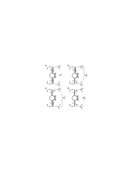
FIG. 1.: Schematic IGM pictures for $(a)$ non-diffractive (ND), $(b)$ and $(c)$ single diffractive (SD) and $(d)$ double Pomeron exchange (DPE) processes.

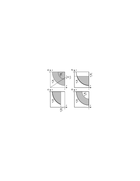
FIG. 2.: Phase space limits of ND, SD and DPE processes in the IGM. The $\frac{1}{2}\ln\frac{x}{y}$ line in a) indicates the rapidity $Y$ of the produced mass $M$.

The hadron-hadron interaction follows the simple picture shown in Fig. 1: the valence quarks fly through essentially undisturbed whereas the gluonic clouds of both projectiles interact strongly with each other forming a central fireball (CF) of mass $M$. The two incoming projectiles $p_{1}$ and $p_{2}$ loose fractions $x$ and $y$ of their original momenta and get excited forming what we call leading jets (LJ’s) carrying $x_{L}=1-x$ and $y_{L}=1-y$ fractions of the initial momenta. Depending on the type of the process under consideration one encounters the different situations depicted in Fig. 1.

In a non-diffractive (ND) process (Fig. 1a) one central fireball of mass $M$ is formed, whereas in single diffractive (SD) events (Figs. 1b and c) the corresponding diffractive systems have masses $M_{X}$ or $M_{Y}$ (comprising also the mass of CF). In double Pomeron exchanges (DPE) (Fig. 1d) a CF of mass $M_{XY}$ is formed. In Fig. 2 we show their corresponding phase space limits. The only difference between ND and SD or DPE processes is that in the latter cases the energy deposition is done by a restricted subset of gluons which in our language is a ”kinematical” Pomeron ($I\!P$), the name which we shall use in what follows.

The central quantity in the IGM is $\chi(x,y)$, the probability to form a CF carrying momentum fractions $x$ and $y$ of two colliding hadrons. It follows from the quantitative implementation of the ideas described above. The essential ingredients are the assumption of multiple independent gluon-gluon collisions, low momentum dominance of the gluon distributions and energy-momentum conservation. The derivation of our main formula, presented below, can be found in Appendix A. $\chi(x,y)$ is given by:

$$\chi(x,y) = \frac{\chi_{0}}{2\pi\sqrt{D_{xy}}}\,\exp\{-\frac{1}{2D_{xy}}[\langle y^{2}\rangle(x-\langle x\rangle)^{2}$$ (1)

$$+ \,\langle x^{2}\rangle(y-\langle y\rangle)^{2}+\,2\,\langle xy\rangle(x-\langle x\rangle)(y-\langle y\rangle)]\}$$ (2)

where $D_{xy}=\langle x^{2}\rangle\langle y^{2}\rangle-\langle xy\rangle^{2}$ and

$$\langle x^{n}\,y^{m}\rangle=\int_{0}^{x_{max}}\!dx^{\prime}\,x^{\prime n}\,\int_{0}^{y_{max}}\!dy^{\prime}\,y^{\prime m}\,\omega(x^{\prime},y^{\prime}),$$ (3)

with $\chi_{0}$ defined by the normalization condition

$$\int_{0}^{1}\!dx\,\int_{0}^{1}\!dy\,\chi(x,y)\,\theta(xy-K_{min}^{2})=1\,,$$ (4)

where $K_{min}=\frac{m_{0}}{\sqrt{s}}$ is the minimal inelasticity defined by the mass $m_{0}$ of the lightest possible CF. The function $\omega(x^{\prime},y^{\prime})$, sometimes called the spectral function, represents the average number of gluon-gluon collisions as a function of $x^{\prime}$ e $y^{\prime}$:

$$\omega(x^{\prime},y^{\prime})\,=\,\frac{d\overline{n}}{dx^{\prime}\,dy^{\prime}}.$$ (5)

The appearance of the number $\overline{n}$ comes from the use of Poissonian distributions, which, in turn, is a consequence of the assumption of independent gluon-gluon collisions. $\omega(x^{\prime},y^{\prime})$ contains all the dynamical inputs of the model both in the perturbative (semihard) and non-perturbative (soft) regimes. The soft and semihard components are given by:

$$\omega^{(S)}(x^{\prime},y^{\prime}) = \frac{\hat{\sigma}^{(S)}_{gg}(x^{\prime}y^{\prime}s)}{\sigma(s)}\,G(x^{\prime})\,G(y^{\prime})$$ (6)

$$\times \theta(x^{\prime}y^{\prime}-{K}_{min}^{2})\,\,\theta(\frac{4\,{p_{T}}_{min}^{2}}{s}-x^{\prime}y^{\prime})$$ (7)

and

$$\omega^{(H)}(x^{\prime},y^{\prime}) = \frac{\hat{\sigma}^{(H)}_{gg}(x^{\prime}y^{\prime}s)}{\sigma(s)}\,G(x^{\prime})\,G(y^{\prime})$$ (8)

$$\times \theta(x^{\prime}y^{\prime}-\frac{4\,{p_{T}}_{min}^{2}}{s})$$ (9)

where $\hat{\sigma}^{S}_{gg}$ and $\hat{\sigma}^{H}_{gg}$ are the soft and semihard gluonic cross sections, $p_{T_{min}}$ is the minimum transverse momentum for minijet production and $\sigma$ denotes the impinging projectiles cross section.

The values of $x_{max}$ and $y_{max}$ depend on the type of the process under consideration. For non-diffractive processes all phase space contained in the shaded area is allowed and in this case we have:

$$x_{max}=y_{max}=1\,\,$$ (10)

The effective number of gluons from the corresponding projectiles are denoted by $G$’s and have been approximated in all our works by the respective gluon distribution functions. There has been a remarkable progress in the knowledge of the parton distributions in hadrons [38, 39, 40], especially in the low $x$ region, which becomes crucial at energies in the TeV range. Since in our previous applications of the IGM we have been studying collisions in the GeV domain, there was no need to use very sophisticated parton distributions. Moreover, very often we needed parton densities at very low scales, which were not considered in the analyses presented in [38, 39, 40]. In some cases, we have used the parametrization of [41], which is better suited for small scales. However, as it will be shown, the IGM can describe both the hadronic and nuclear collision data with the following simple form of the gluon distribution function in the nucleon:

$$G(x)=p(m+1)\,\frac{(1-x)^{m}}{x}$$ (11)

with $m=5$ and the fraction of the energy-momentum allocated to gluons is equal to $p=0.5$.

In the IGM picture, diffractive and non-diffractive events have been treated on the same footing in terms of gluon-gluon collisions. Single diffractive processes receive great attention mainly because of their potential ability to provide information about the most important object in the Regge theory, namely the Pomeron ($I\!P$), its quark-gluon structure and cross sections. As can be seen in Fig. 1b (1c), the ”diffractive mass” $M_{X}$ ($M_{Y}$) is just the invariant mass of a system composed of the CF and LJ formed by one of the colliding projectiles. The main difference with the ”non-diffractive mass” $M$ in Fig. 1a is that the energy transfer from the diffracted projectile is now done by the highly correlated subset of gluons (denoted by $I\!P$) which are supposed to be in a color singlet state. In technical terms it means that in comparison to the previous applications of the IGM cited before, we are free to change both the possible shape of the function $G(x)$ ($\equiv G_{I\!P}(x)$), the number of gluons participating in the process and the cross section $\sigma$ ($\equiv\sigma_{pI\!P}$) in the spectral function $\omega$ used above. The function $G_{I\!P}(x)$ should not be confused with the momentum distribution of the gluons inside the Pomeron, $f_{g/I\!P}(\beta)$. The former is given by the convolution of the latter with the Pomeron flux factor as discussed in the Appendix B. Actually we have found that we can keep the shape of $G(x)$ the same as before and the only change necessary to reach agreement with data is the amount of energy-momentum $p=p_{I\!P}$ allocated to the impinging hadron and which will find its way in the object that we call $I\!P$. It turns out that $p_{I\!P}\simeq 0.05$, whereas $p\simeq 0.5$ for all gluons encountered so far. This choice, with $m=5$ in eq. (11), corresponds to an intermediate between “soft” and “hard” Pomeron (see Appendix B) and will be used in what follows. Just in order to make use of the present knowledge about the Pomeron, we have chosen $\sigma(s)=\sigma_{pI\!P}\,=\,a+b\,\ln(s/s_{0})$ where $s_{0}=1$ $GeV^{2}$ and $a=2.6$ $mb$ and $b=0.01$ $mb$.

In single diffractive processes only a limited part of the phase space supporting the $\chi(x,y)$ distribution is allowed and in this case the integration limits in the moments of the spectral function $\omega$ (eq. (3)) depend on the mass $M_{X}$ or $M_{Y}$ that is produced:

$$x_{max}=1\,\,\,;\,\,\,y_{max}=y\,\,\,;\,\,\,x_{max}\,y_{max}=M_{X}^{2}/s$$ (12)

$$x_{max}=x\,\,\,;\,\,\,y_{max}=1\,\,\,;\,\,\,x_{max}\,y_{max}=M_{Y}^{2}/s$$ (13)

By reducing these maximal values we select events in which the energy released by the projectile emitting $I\!P$ is small and at the same time allow the formation of a rapidity gap betwen the diffractive mass and the diffracted projectile. This is the experimental requirement defining a SD event.

Double Pomeron Exchange processes, inspite of their small cross sections, are inclusive measurements and do not involve particle identification, dealing only with energy flow. Such a process was recently measured by UA8 [24] and used to deduce the $I\!PI\!P$ cross section, $\sigma_{I\!PI\!P}$. It turned out that using this method one gets $\sigma_{I\!PI\!P}$ which apparently depends on the produced mass $M_{XY}$. This fact was tentatively interpreted as signal of glueball formation [24]. In the IGM a double Pomeron exchange event (Fig. 1d) is seen as a specific type of energy flow. The difference between it and the ”normal” energy flow as represented by Fig. 1a is that now the gluons involved in this process must be confined to the object we called $I\!P$ above. We are implicitly assuming that all gluons from $p_{1}$ and $p_{2}$ participating in the collision (i.e., those emitted from the upper and lower vertex in Fig. 1d) have to form a color singlet. In this case two large rapidity gaps will form separating the diffracted hadron $p_{1}$, the $M_{XY}$ system and the diffracted hadron $p_{2}$, which is the experimental requirement defining a DPE event. Also in this case only a limited part of the phase space supporting the $\chi(x,y)$ distribution is allowed and the limits in the moments of the spectral function $\omega$ (eq. (3)) depend on the mass $M_{XY}$ in the following way:

$$x_{max}=x\,\,\,;\,\,\,y_{max}=y\,\,\,;\,\,\,x_{max}\,y_{max}=M_{XY}^{2}/s\,.$$ (14)

As before $G_{I\!P}(x)$ represent the number of gluons participating in the process and the cross section $\sigma$, appearing in eqs. (7) and (9), represents now the Pomeron-Pomeron cross section, $\sigma_{I\!PI\!P}$.

The clear separation between valence quarks and bosonic degrees of freedom does not appear exclusively in the IGM. It appears also in soliton models of the nucleon [42]. In the Chiral Quark Soliton Model [43], for example, the nucleon is made of three massive quarks bound by the self-consistent pion field (the ”soliton”). It is interesting to observe that, according to this model, in a collision of two nucleons the valence quarks would interact much less than the pions and therefore would filter through and populate the large rapidity regions leaving behind a blob of pionic matter in the central region.

III Inelasticity

The energy dependence of inelasticity is an important problem which is still subject of debate [44]. Generally speaking, inelasticity $K$ is the fraction of the total energy carried by the produced particles in a given collision. However in the literature one finds several possible ways to define it. In the first one, inelasticity is defined as

$$K_{1}\,=\,\frac{M}{\sqrt{s}}$$ (15)

where $\sqrt{s}$ is the total reaction energy in its center of mass frame and $M$ is the mass of the system (fireball, string, etc.) which decays into the final produced particles. The second definition of $K$ considered here is

$$K_{2}\,=\,\frac{1}{\sqrt{s}}\,\sum_{i}\int dy\,\mu_{i}\,\frac{dn_{i}}{dy}\,\cosh y$$ (16)

where $\mu_{i}=\sqrt{p_{{\scriptscriptstyle T}_{i}}^{2}+m^{2}_{i}}$ is the transverse mass of the produced particles of type $i$ and $dn_{i}/dy$ their measured rapidity distribution. These two definitions are, in principle, model independent, although the mass $M$ might be difficult to evaluate in certain models.

The main difference between $K_{1}$ and $K_{2}$ is that, whereas the first one refers to partons, the second one refers to final observed hadrons. $K_{2}$ implicitly includes the kinetic energy of the object of mass $M$. From the theoretical point of view, $K_{1}$ is a very interesting quantity because it can be easy to calculate and because it is the relevant quantity when studying the formation of dense systems (e.g. quark-gluon plasma).

In Ref. [12] we used the IGM to study the energy dependence of $K_{1}$. We concluded that the introduction of a semihard component (minijets) in that model produces increasing inelasticities at the partonic level. In Ref. [13] we introduced a hadronization mechanism in the IGM, calculated the rapidity distributions of the produced particles, compared our results with the UA5 and UA7 data and finally calculated $K_{2}$. The purpose of this exercise was to verify whether the hadronization process changed our previous conclusion. We found that, whereas some quantitative aspects, like the existence or not of Feynman Scaling in the fragmentation region and the numerical values of $K_{2}$, depend very strongly on details of the fragmentation process, the statement that minijets lead to increasing inelasticities remains valid.

In Fig. 3 we show the IGM pseudorapidity distributions compared to UA5 data at different energies [45] and CDF [46] data at $\sqrt{s}=1800$ GeV. For the sake of comparison with other models based both on soft and semihard dynamics, we show in Fig. 4 our results for the multiplicity (Fig. 4a) and central rapidity density (Fig. 4b) together with the results of HIJING [1] for the same quantities.

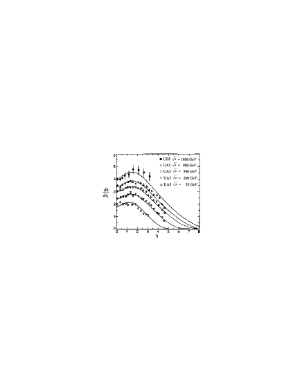
FIG. 3.: Pseudorapidity distributions measured at the central rapidity region. Data are from the UA5 collaboration [45] at different energies and from CDF collaboration [46] at $\sqrt{s}=1800$ GeV. Full lines show the IGM results.

Both models fit the data but differ significantly when one switches off the semihard (minijet) contribution. Whereas in HIJING Feynman Scaling violation in the central region (the growth of  ${\displaystyle\left.dn/d\eta\right|_{\eta=0}}$  with  $\sqrt{s}\,$) is entirely due to the minijets, in the IGM this behavior is partly due to soft interactions, there being only a quantitative difference when minijets are included.

In Fig. 5 we plot $K_{2}$ (full lines) and $K_{1}$ (dashed lines as a function of $\sqrt{s}$. The lower curves show the results when minijets are switched off and only soft interactions take place. The upper curves show the effect of including minijets.

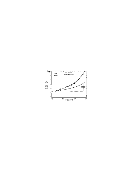
FIG. 4.: a) Average charged multiplicities as a function of the reaction energy. Squares and circles are experimental data. Full lines show the IGM results with and without the semihard contribution (lower curve). Dashed lines show the same quantities calculated with HIJING [1]. b) The same as a) for the central pseudorapidity distribution ${\displaystyle\left.dn/d\eta\right|_{\eta=0}}$.

IV Leading charm and beauty

In Ref. [14] we treated leading charm production in connection with energy deposition in the central rapidity region giving special attention to the correlation between production in central and fragmentation regions. The significant difference between the $x_{F}$ dependence of leading and nonleading charmed mesons [47] was not possible to be explained with the usual perturbative QCD [48] or with the string fragmentation model contained in PYTHIA [49].

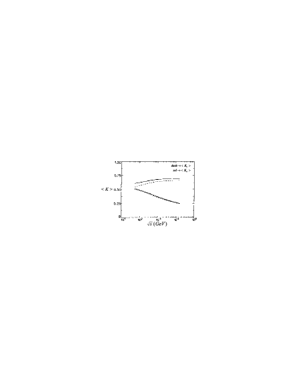
FIG. 5.: Inelasticities $K_{1}$ (dashed lines) and $K_{2}$ (solid lines) with minijets (upper curves) and without minijets (lower curves) as a function of the reaction energy.

In the case of pion-nucleon scattering, the measured leading charmed mesons [47] are $D^{-}$ and the nonleading are $D^{+}$. In the spirit of IGM, the central production ignores the valence quarks of target and projectile which, in the first approximation, just “fly through”. Because of this, the centrally produced $D$’s do not show any leading particle effect. There are, however, two distinct ways to produce $D$ mesons out of LJ’s: fragmentation and recombination. We assumed that, whenever energy allows, we would have also $\bar{c}c$ pairs in the LJ (produced, for example, from the remnant gluons present there). These charmed quarks might undergo fragmentation into $D$ mesons and also recombine with the valence quarks. Whereas $D^{+}$ and $D^{-}$ mesons are equally produced via fragmentation only ”leading” $D^{-}$’s (which carry the valence quarks of target and projectile) can be produced by recombination. It turns out that only this last process will produce asymmetry.

The idea that $\bar{c}c$ pairs pre-exist in the projectiles can be made more precise and the origin of these “intrinsic charm” pairs can be attributed to the existence of a meson cloud around the nucleons and pions [50].

The asymmetry in $D$ meson production can be defined as:

$$A(x_{F}) = \frac{\frac{d\sigma^{D^{-}}(x_{F})}{dx_{F}}\,\,-\,\,\frac{d\sigma^{D^{+}}(x_{F})}{dx_{F}}}{\frac{d\sigma^{D^{-}}(x_{F})}{dx_{F}}\,\,+\,\,\frac{d\sigma^{D^{+}}(x_{F})}{dx_{F}}}$$ (17)

In Fig. 6 we compare our calculations with experimental data from the WA82, E769 and E791 [47] collaborations. The main conclusion of the work is that if one takes properly into account the correlation between energy deposition in the central region and the leading particle momentum distribution, at higher energies the increase of inelasticity will lead to the decrease of the asymmetry in heavy quark production. In other words, if the fraction of the reaction energy released in the central region increases the asymmetry in the $x_{F}$ distributions of charmed mesons will become smaller. In Fig. 7 we illustrate this quantitatively and also consider the leading beauty production.

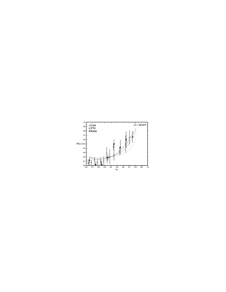
FIG. 6.: Asymmetry calculated with the IGM and compared with WA82 (solid circles), with E769 (open squares) and E791 (open triangles) data [47]. Solid, dashed and dotted lines correspond to different weights of the recombination component equal to 80%, 50% and 20% respectively.

FIG. 7.: $B^{-}$/$B^{+}$ (solid lines) and $D^{-}$/$D^{+}$ (dashed lines) asymmetries at $\sqrt{s}=$ 26 and 1800 GeV.

V Diffractive mass spectra in hadron-hadron collisions

Diffractive scattering processes have received increasing attention for several reasons. They are also related to the large rapidity gap physics and the structure of the Pomeron. In a diffractive scattering, one of the incoming hadrons emerges from the collision only slightly deflected and there is a large rapidity gap between it and the other final state particles resulted from the other excited hadron. Diffraction is due to the Pomeron exchange but the exact nature of the Pomeron in QCD is not yet elucidated. The first test of a model of diffractive dissociation (SD) is the ability to properly describe the mass ($M_{X}$) distribution of diffractive systems, which has been measured in many experiments [51] and parametrized as $(M_{X}^{2})^{-\alpha}$ with $\alpha\simeq 1$.

In Ref. [15] we studied diffractive mass distributions using the Interacting Gluon Model focusing on their energy dependence and their connection with inelasticity distributions. One advantage of the IGM is that it was designed in such a way that the energy-momentum conservation is taken care of before all other dynamical aspects. This feature makes it very appropriate for the study of energy flow in high energy hadronic and nuclear reactions. As mentioned before, in our approach the definition of the object $I\!P$ (see Fig. 1b and c) is essentially kinematical, very much in the spirit of those used in other works which deal with diffractive processes in the parton and/or string language. In order to regard our process as being of the SD type we simply assume that all gluons from the target hadron participating in the collision (i.e., those emitted from the lower vertex in Fig. 1b) have to form a colour singlet. Only then a large rapidity gap will form separating the diffracted hadron and the $M_{X}$ system. Otherwise a colour string would develop, connecting the diffracted hadron and the diffractive cluster, and would eventually decay, filling the rapidity gap with produced secondaries. As was said above, it is a special class of events in which the energy released by the projectile emiting $I\!P$ is small and consequently the diffractive mass is small. Once only a limited part of the phase space is allowed, the limits in the moments of the spectral function $\omega$ (eq. (3)), depend on the mass $M_{X}$ that is produced through the constraint $y_{max}=y=M_{X}^{2}/s$ (see eq. (12)).

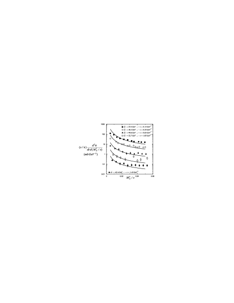
FIG. 8.: Diffractive mass spectrum for $pp$ collisions calculted with the IGM and compared with CERN-ISR data [52].

As shown in Appendix A, the mass spectra for SD processes is given by:

$$\frac{1}{\sigma}\frac{d\sigma}{dM_{X}^{2}} = \frac{dN}{dM_{X}^{2}}=\int_{0}^{1}dx\,\int_{0}^{1}dy\,\chi(x,y)$$ (18)

$$\times \,\delta\left(M^{2}_{X}-sy\right)\,\theta\left(xy-K_{min}^{2}\right)$$ (19)

Although in the final numerical calculations the above complete formulation is used, it is worthwhile to present approximate analytical results in order to illustrate the main characteristic features of the IGM diffractive dissociation processes. By keeping only the most singular terms in gluon distribution functions, i.e., $G(x)\simeq\frac{1}{x}$ and only the leading terms in $\sqrt{s}$, as shown in Appendix A, we arrive at the following expression:

$$\frac{dN}{dM_{X}^{2}}\, \simeq \,\frac{1}{s}\,H(M_{X}^{2},s)\,F(M^{2}_{X},s)$$ (20)

$$\simeq \,\frac{\rm const}{M_{X}^{2}}\,\frac{1}{\sqrt{c\,\ln\frac{M_{X}^{2}}{m_{0}^{2}}}}\,\exp\left[-\frac{\left(1\,-\,c\,\ln\frac{M_{X}^{2}}{m_{0}^{2}}\right)^{2}}{c\,\ln\frac{M_{X}^{2}}{m_{0}^{2}}}\right].$$ (21)

where $c$ is a constant and $m_{0}$ is a soft energy scale. The expression above is governed by the $\frac{1}{M^{2}_{X}}$ term. The other two terms have a weaker dependence on $M^{2}_{X}$. They distort the main ($\frac{1}{M^{2}_{X}}$) curve in opposite directions and tend to compensate each other. It is therefore very interesting to note that even before choosing a very detailed form for the gluon distributions and hadronic cross sections we obtain analytically the typical shape of a diffractive spectrum, $\frac{1}{M^{2}_{X}}$.

In Fig. 8 we show our diffractive mass spectrum and compare it to experimental data from the CERN-ISR [52]. Fig. 9 shows the diffractive mass spectrum for $\sqrt{s}=1800$ GeV compared to experimental data from the E710 Collaboration [53]. In these curves we have used our intermediate Pomeron profile: $G_{I\!P}(y)$ given by (11) with $m=5$ and $p_{{I\!P}}=0.05$.

In all curves we observe a modest narrowing as the energy increases. This small effect means that the diffractive mass becomes a smaller fraction of the available energy $\sqrt{s}$. In other words, the ”diffractive inelasticity” decreases with energy and consequently the ”diffracted leading particles” follow a harder $x_{F}$ spectrum. Physically, in the context of the IGM, this means that the deposited energy is increasing with $\sqrt{s}$ but it will be mostly released outside the phase space region that we are selecting. A measure of the ”diffractive inelasticity” is the quantity $\xi=M^{2}_{X}/s$. It is very simple to calculate its average value $\langle\xi\rangle$ from the diffractive mass spectrum. Making a trivial change of variables we get:

$$\langle\xi\rangle\left(s\right) = \int_{\xi_{min}}^{\xi_{max}}d\xi\,\frac{dN}{d\xi}\,\xi$$ (22)

where $\xi_{min}$ ($=1.5/s$) and $\xi_{max}$ ($=0.1$) are the same used in other works. In Fig. 10 we plot $\langle\xi\rangle$ against $\sqrt{s}$. As it can be seen $\langle\xi\rangle$ decreases with $\sqrt{s}$ not only because $\xi_{min}$ becomes smaller but also because $dN/d\xi$ changes with the energy, falling faster. Also shown in Fig. 10 is the quantity $\langle\xi^{\varepsilon}\rangle$ (sometimes used in connection with the energy dependence of the single diffractive cross-section) for $\varepsilon=0.08$ (dashed lines) and $\varepsilon=0.112$ (dotted lines).

FIG. 9.: Diffractive mass spectrum for $p\bar{p}$ collisions calculted with the IGM and compared with FERMILAB Tevatron data [53].

FIG. 10.: Energy dependence of the ”diffractive inelasticity” $\langle\xi\rangle$ and of $\langle\xi^{\varepsilon}\rangle$.

VI Diffractive mass spectra in electron-hadron collisions

At the HERA electron-proton collider the bulk of the cross section corresponds to photoproduction, in which a beam electron is scattered through a very small angle and a quasi-real photon interacts with the proton. For such small virtualities the dominant interaction mechanism takes place via fluctuation of the photon into a hadronic state (vector meson dominance) which interacts with the proton via the strong force. High energy photoproduction therefore exhibits similar characteristics to hadron-hadron interactions.

In Ref. [16] we studied diffractive mass distributions in a photon-proton collision. The photon is converted into a mesonic state and then interacts with the incoming proton. The diffractive meson-proton interaction follows then the usual IGM picture. The diffracted proton in Fig. 1b), looses only a fraction $y$ of its momentum but otherwise remains intact. In the limit $y\rightarrow 1$, the whole available energy is stored in $M_{X}$ which then remains at rest, i.e., $Y_{X}=0$. For small values of $y$ we have small masses $M_{X}$ located at large rapidities $Y_{X}$. As before the upper cut-off $y_{max}$ ($=y=M_{X}^{2}/s$) is a kinematical restriction preventing the gluons coming from the diffracted proton (and forming our object $I\!P$) to carry more energy than what is released in the diffractive system. It plays a central role in the adaptation of the IGM to diffractive dissociation processes being responsible for its proper $M^{2}_{X}$ dependence.

FIG. 11.: Diffractive mass spectrum for $\gamma p$ collisions at $W=187\,GeV$ calculted with the IGM and compared with H1 data [54]. The different curves correspond to the choices: I ($m_{0}=0.31\,GeV$, $\sigma=2.7\,mb$), II ($m_{0}=0.35\,GeV$, $\sigma=2.7\,mb$), III ($m_{0}=0.31\,GeV$, $\sigma=5.4\,mb$) and IV ($m_{0}=0.35\,GeV$, $\sigma=5.4\,mb$), respectively.

In the upper leg of Fig. 1b) we have assumed, for simplicity, the vector meson to be $\rho^{0}$ and take $G^{\rho^{0}}(x)=G^{\pi}(x)$. Since the parameter $p/\sigma$ appearing in eqs. (7) and (9) has been fixed considering the proton-proton diffractive dissociation and here we are addressing the $p\rho^{0}$ case there exists some freedom to change $\sigma$. We can also investigate the effect of small changes in the value of $m_{0}$ on our final results.

FIG. 12.: Diffractive mass spectrum for $\gamma p$ collisions at $W=187\,GeV$ calculted with the IGM and compared with H1 data [54]. The solid line (curve II) corresponds to the choice $m_{0}=0.35\,GeV$, $\sigma=2.7\,mb$ and $G_{I\!P}(y)$. Curves I (dashed) and III (dotted) are obtained replacing $G_{I\!P}(y)$ by $G^{h}_{I\!P}(y)$ and $G^{s}_{I\!P}(y)$ respectively. Curve IV is obtained with $G^{s}_{I\!P}(y)$ and $m_{0}=0.50\,GeV$ and $\sigma=5.4\,mb$.

In Fig. 11 we compare our results, eq. (19), for different choices of $m_{0}$ and $\sigma$ with the data from the H1 collaboration [54]. In all these curves we have used our intermediate Pomeron profile. In Fig. 12 we compare the same data with our mass spectrum obtained with $G^{h}_{I\!P}(y)$ (curve I), $G_{I\!P}(y)$ (curve II) and $G^{s}_{I\!P}(y)$ (curve III). This comparison suggests that the “hard” Pomeron can give a good description of data. The same can be said about our “mixed” Pomeron, which, in fact seems to be more hard than soft. These three curves were calculated with exactly the same parameters and normalizations, the only difference being the Pomeron profile. Soft and hard gluon distributions $G^{s,h}_{I\!P}(y)$ are calculated in the Appendix B. Apparently the “soft” Pomeron (curve III) is ruled out by data.

VII Diffractive mass spectra in double Pomeron exchange

After ten years of work at HERA, an impressive amount of knowledge about the Pomeron has been accumulated, especially about its partonic composition and parton distribution functions. Less known are its interaction properties. Whereas the Pomeron-nucleon cross section has been often discussed in the literature, the recently published data by the UA8 Collaboration [24] have shed some light on the Pomeron-Pomeron interaction. In [24] the Double Pomeron Exchange cross section was written as the product of two flux factors with the $I\!PI\!P$ cross section, $\sigma_{I\!PI\!P}$, being thus directly proportional to this quantity. This simple formula relies on the validity of the Triple-Regge model, on the universality of the Pomeron flux factor and on the existence of a factorization formula for DPE processes. However, for these processes the factorization hypothesis has not been proven and is still matter of debate [55, 56, 57, 58]. In [59] it was shown that factorizing and non-factorizing DPE models may be experimentally distinguished in the case of dijet production.

Fitting the measured mass spectra allowed for the determination of $\sigma_{I\!PI\!P}$ and its dependence on $M_{X}$, the mass of the diffractive system. The first observation of the UA8 analysis was that the measured diffractive mass ($M_{X}$) spectra show an excess at low values that can hardly be explained with a constant (i.e., independent of $M_{X}$) $\sigma_{I\!PI\!P}$. Even after introducing some mass dependence in $\sigma_{I\!PI\!P}$ they were not able to fit the spectra in a satisfactory way. Their conclusion was that the low $M_{X}$ excess may have some physical origin like, for example glueball formation.

Although the analysis performed in [24] is standard, it is nevertheless useful to confront it with the IGM description of the diffractive interaction. Double Pomeron exchange processes, inspite of their small cross sections, appear to be an excellent testing ground for the IGM because they are inclusive measurements and do not involve particle identification, dealing only with energy flow. In Ref. [25] we studied the diffractive mass distribution observed by UA8 Collaboration in the inclusive reaction $p\bar{p}\rightarrow pX\bar{p}$ at $\sqrt{s}=630\,GeV$, using the IGM with DPE included. The interaction follows the picture shown in Fig. 1d.

As shown in Appendix A, the mass spectrum for DPE processes is given by:

$$\frac{1}{\sigma}\frac{d\sigma}{dM_{XY}} = \frac{dN}{dM_{XY}}=\int_{0}^{1}dx\,\int_{0}^{1}dy\,\chi(x,y)$$ (23)

$$\times \,\delta\left(M_{XY}-\sqrt{xys}\right)\,\theta\left(xy-K_{min}^{2}\right)$$ (24)

As indicated in the recent literature [55, 56, 57, 58, 59], one of the crucial issues in diffractive physics is the possible breakdown of factorization. As stated in [56] one may have Regge and hard factorization. Our model does not rely on any of them. In the language used in [56], we need and use a “diffractive parton distribution” and we do not really need to talk about “flux factor” or “distribution of partons in the Pomeron”. Therefore there is no Regge factorization implied. However, we will do this connection in eq. (B6) of the Appendix B, in order to make contact with the Pomeron pdf’s parametrized by the H1 and ZEUS collaborations. As for hard factorization, it is valid as long as the scale $\mu$ is large. In the IGM, as it will be seen, the scale is given by $\mu^{2}=xys$, a number which sometimes is larger than $3-4\,GeV^{2}$ but sometimes is smaller, going down to values only slightly above $\Lambda_{QCD}^{2}$. When the scale is large ($\mu^{2}>p_{T_{mim}}^{2}$) we employ Eq. (9) and when it is smaller ($m^{2}_{0}<\mu^{2}<p_{T_{mim}}^{2}$) we use Eq. (7). Therefore, in part of the phase space we are inside the validity domain of hard factorization, but very often we are outside this domain. From the practical point of view, Eq. (9), being defined at a semihard scale, relies on hard factorization for the elementary $gg\rightarrow gg$ interaction, uses parton distribution function extracted from DIS and an elementary cross section $\hat{\sigma}_{gg}$ taken from standard pQCD calculations. The validity of the factorizing-like formula Eq. (7) is an assumption of the model. In fact, the relevant scale there is $m_{0}^{2}\simeq\Lambda_{QCD}^{2}$ and, strictly speaking, there are no rigorously defined parton distributions, neither elementary cross sections. However, using Eq. (7) has non-trivial consequences which were in the past years supported by an extensive comparison with experimental data. In this approach, since we have fixed all parameters using previous data on leading particle formation and single diffractive mass spectra, there are no free parameters here, except $\sigma_{I\!PI\!P}$.

We start evaluating Eq. (24) with the inputs that were already fixed by other applications of the IGM, namely, (B7) with $p_{d}=0.05$. In Fig. 13 we show the numerical results for DPE mass distribution normalized to the “AND” data sample of [24]. We have fixed the parameter $\sigma$ ($\equiv\sigma_{I\!\!PI\!\!P}$) appearing in Eq. (7) and Eq. (9), to $0.5\,mb$ (dashed lines) and $1.0\,mb$ (solid lines).

We emphasize that, in this approach, since we have fixed all parameters using previous data on leading particle formation and single diffractive mass spectra, there are no free parameters here, except $\sigma_{I\!\!PI\!\!P}$. As it can be seen from the figure, in our model we obtain the fast increase of spectra in the low mass region without the use of a $M_{X}$ dependent $I\!\!P$ $I\!\!P$ cross section and this quantity seems to be approximately $\sigma_{I\!\!PI\!\!P}\simeq 0.5\,mb$.

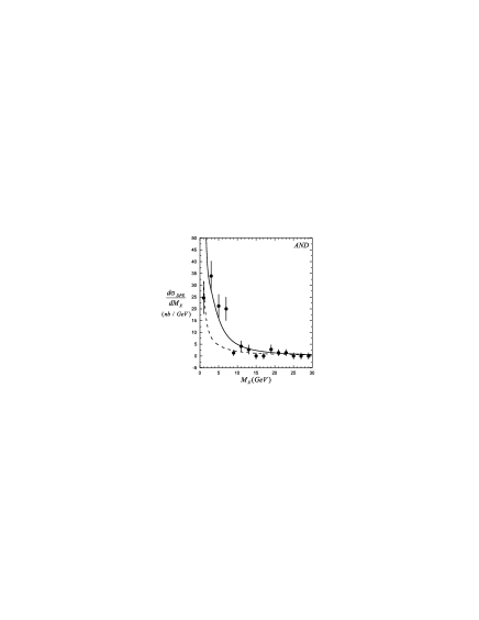
FIG. 13.: IGM DPE diffractive mass distributions: Solid and dashed lines show the results with $\sigma_{I\!PI\!P}$ equal to $0.5\,mb$ and $1.0\,mb$, respectively, calculated with the intermediate Pomeron profile. Our curves were normalized to the “AND” data sample of [24].

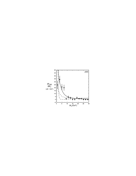
FIG. 14.: IGM DPE diffractive mass distributions: Solid line as in Fig. 13, dashed and dash-dotted lines represent the “hard” and “super-hard” Pomeron profiles. In all cases $\sigma_{I\!PI\!P}=0.5\,mb$. Our curves were normalized to the “AND” data sample of [24].

We next replace (B7) by the convolution (B6) to see which of the previously considered Pomeron profiles, hard or superhard, gives the best fit of the UA8 data. In doing so, we shall keep everything else the same, i.e., $p_{d}=0.05$ and $\sigma_{I\!\!PI\!\!P}=0.5\,mb$.

In Fig. 14, we repeat the fitting procedure used in Fig. 13 for these Pomeron profiles. Solid, dashed and dash-dotted lines represent respectively Eq. (B7), hard and superhard Pomerons. We see that, for harder Pomeron profiles we “dig a hole” in the low mass region of the spectrum. Note that the solid lines are the same as in Fig. 13. Looking at the figure, at first sight, we might be tempted to say that Eq. (B7) gives the best agreement with data and a somewhat worse description can be obtained with the hard Pomeron (in dashed lines), the superhard being discarded. However, comparing the dashed lines in Fig. 13 and Fig. 14 and observing that they practically coincide with each other, we conclude that the same curve can be obtained either with (B7) and $\sigma_{I\!\!PI\!\!P}=1.0\,mb$ (dashed line in Fig. 13) or with (B6), (B2) and $\sigma_{I\!\!PI\!\!P}=0.5\,mb$ (dashed line in Fig. 14). In other words we can trade the “hardness” of the Pomeron with its interaction cross section. The following two objects give an equally good description of data: i) a Pomeron composed by more and softer gluons and with a larger cross section and ii) a Pomeron made by fewer, harder gluons with a smaller interaction cross section. We have checked that this reasoning can be extended to the superhard Pomeron. Although, apparently disfavoured by Fig. 14 (dash-dotted lines), it might still fit the data provided that $\sigma_{I\!\!PI\!\!P}<0.25\,mb$. Given the uncertainties in the data and the limitations of the model, we will not try for the moment to refine this analysis. It seems possible to describe data in a number of different ways. We conclude then that nothing exotic has been observed and also that the Pomeron-Pomeron cross section is bounded to be $\sigma_{I\!\!PI\!\!P}<1.0\,mb$.

FIG. 15.: IGM prediction for $d\sigma/dM_{X}$ at LHC with $\sigma_{I\!PI\!P}=1.0\,mb$. Cross($+$) and Cross($\times$) are predictions made by Brandt et al. [24] for two values of effective Pomeron intercepts $\alpha(0)=1+\varepsilon$.

In Fig. 15 we compare our predictions for $d\sigma/dM_{X}$ (mb/GeV) for LHC ($\sqrt{s}=14$ TeV) assuming an $M_{X}$-independent $\sigma_{I\!\!PI\!\!P}=1.0\,mb$ (and using (B7)) with predictions made by Brandt et al. [24] for two values of effective Pomeron intercepts ($\alpha(0)=1+\varepsilon$), $\varepsilon=0.0$ and $0.035$.

FIG. 16.: Ratio double/single Pomeron exchange mass distributions as a function of $M_{X}$. In both cases we have assumed $\sigma_{I\!\!PI\!\!P}=1.0\,mb$ (for DPE processes) and $\sigma_{pI\!\!P}=1.0\,mb$ (for SPE processes).

Although the normalization of our curves is arbitrary, the comparison of the shapes reveals a difference between the two predictions. Whereas the points (from [24]) show spectra broadening with the c.m.s. energy, we predict (solid line) the opposite behavior: as the energy increases we observe a (modest) narrowing for $d\sigma/dM_{X}$. This small effect means that the diffractive mass becomes a smaller fraction of the available energy $\sqrt{s}$. In other words, the “double diffractive inelasticity” decreases with energy in the same way as the “diffractive inelasticity”, as seen in Fig. 10.

We are not able to make precise statements about the diffractive cross section (in particular about its normalization) with our simple model. Nevertheless, the narrowing of $d\sigma_{DPE}/dM_{X}$ suggests a slower increase (with $\sqrt{s}$) of the integrated distribution $\sigma_{DPE}$. We found this same effect also for $\sigma_{SPE}$. This trend is welcome and is one of the possible mechanisms responsible for the suppression of diffractive cross sections at higher energies relative to some Regge theory predictions.

In Fig. 16 we show the ratio $R(M_{X})$ defined by:

$$R(M_{X})=\frac{\frac{1}{\sigma_{DPE}}\,\frac{d\sigma_{DPE}}{dM_{X}}}{\frac{1}{\sigma_{SPE}}\,\frac{d\sigma_{SPE}}{dM_{X}}}$$ (25)

This quantity involves only distributions previously normalized to unity and does not directly compare the cross sections (which are numerically very different for DPE and single diffraction). In $R$ the dominant $1/M^{2}_{X}$ factors cancel and we can better analyse the details of the distributions which may contain interesting dynamical information. The most prominent feature of Fig. 16 is the rise of the ratio with $M_{X}$, almost by one order of magnitude in the mass range considered. This can be qualitatively attributed to the fact that, in single diffractive events the object $X$ has larger rapidities than the corresponding cluster formed in DPE events. As a consequence, when energy is released from the incoming particles in a SPE event, it goes more to kinetic energy of the $X$ system (i.e., larger momentum $P_{X}$ and rapidity $Y_{X}$) and less to its mass. In DPE, although less energy is released, it goes predominantly to the mass $M_{X}$ of the difractive cluster, which is then at lower values of $Y_{X}$. In order to illustrate this behavior, we show in Fig. 17 the rapidity distributions of the $X$ (which has mass $M_{X}$) and $XY$ (which has mass $M_{XY}$) systems. All curves are normalized to unity and with them we just want to draw attention to the dramatically different positions of the maxima of these distributions. The solid and dashed lines show $1/\sigma\,d\sigma/dY_{X}$ for DPE (curves on the left) and SPE (curves on the right) computed at $\sqrt{s}=630\,GeV$ and $\sqrt{s}=2000\,GeV$, respectively. We can clearly observe that DPE and SPE rapidity distributions are separated by three units of rapidity and this difference stays nearly constant as the c.m.s. energy increases. The location of maxima in $1/\sigma\,d\sigma/dY_{X}$ and their energy dependence are predictions of our model.

FIG. 17.: Double and single Pomeron exchange normalized rapidity ($Y_{X}$) distributions. In both cases we have assumed $\sigma_{I\!\!PI\!\!P}=1.0\,mb$ (for DPE processes) and $\sigma_{pI\!\!P}=1.0\,mb$ (for SPE processes).

VIII Leading particle spectra

The leading particle effect is one of the most interesting features of multiparticle production in hadron-hadron collisions. In high energy hadron-hadron collisions the momentum spectra of outgoing particles which have the same quantum numbers as the incoming particles, also called leading particle (LP) spectra, have been measured already some time ago [60, 61]. Later on, new data on pion-proton collisions were released by the EHS/NA22 collaboration [62] in which the spectra of both outcoming leading particles, the pion and the proton, were simultaneously measured. More recently data on leading protons produced in eletron-proton reactions at HERA with a c.m.s. energy one order of magnitude higher than in the other above mentioned hadronic experiments became available [63]. In the case of photoproduction, data can be interpreted in terms of the Vector Dominance Model [64] and can therefore be considered as data on LP production in vector meson-proton collisions. These new measurements of LP spectra both in hadron-hadron and in eletron-proton collisions have renewed the interest on the subject, specially because the latter are measured at higher energies and therefore the energy dependence of the LP spectra can now be determined.

It is important to have a very good understanding of these spectra for a number of reasons. They are the input for calculations of the LP spectra in hadron-nucleus collisions, which are a fundamental tool in the description of atmospheric cascades initiated by cosmic radiation [9, 65]. There are several new projects in cosmic ray physics including the High Resolution Fly’s Eye Project, the Telescope Array Project and the Pierre Auger Project [66] for which a precise knowledge of energy flow (LP spectra and inelasticity distributions) in very high energy collisions would be very useful.

In a very different scenario, namely in high energy heavy ion collisions at RHIC, it is very important to know where the outgoing (leading) baryons are located in momentum space. If the stopping is large they will stay in the central rapidity region and affect the dynamics there, generating, for example, a baryon rich equation of state. Alternatively, if they populate the fragmentation region, the central (and presumably hot and dense) region will be dominated by mesonic degrees of freedom. The composition of the dense matter is therefore relevant for the study of quark gluon plasma formation [8].

In any case, before modelling $p-A$ or $A-A$ collisions one has to understand properly hadron-hadron processes. The LP spectra are also interesting for the study of diffractive reactions, which dominate the large $x_{F}$ region.

Since LP spectra are measured in reactions with low momentum transfer and go up to large $x_{F}$ values, it is clear that the processes in question occur in the non-perturbative domain of QCD. One needs then “QCD inspired” models and the most popular are string models, like FRITIOF, VENUS or the Quark Gluon String Model (QGSM). Calculation of LP spectra involving these models can be found in Refs. [67] and [68].

A Leading particles in hadron-hadron collisions

In the framework of the QCD parton model of high energy collisions, leading particles originate from the emerging fast partons of the collision debris. There is a large rapidity separation between fast partons and sea partons. Fast partons interact rarely with the surrounding wee partons. The interaction between the hadron projectile and the target is primarily through wee parton clouds. A fast parton or a coherent configuration of fast partons may therefore filter through essentially unaltered. Based on these observations and aiming to study $p-A$ collisons, the authors of Ref. [67] proposed a mechanism for LP production in which the LP spectrum is given by the convolution of the parton momentum distribution in the projectile hadron with its corresponding fragmentation function into a final leading hadron. This independent fragmentation scheme is, however, not supported by leading charm production in pion-nucleus scattering. It fails specially in describing the $D^{-}/D^{+}$ asymmetry. A number of models addressed these data and the conclusion was that valence quark recombination is needed. Translated to leading pion or proton production this means that what happens is rather a coalescence of valence quarks to form the LP and not an independent fragmentation of a quark or diquark to a pion or a nucleon. Another point is that the coherent configuration formed by the valence quarks may go through the target but, due to the strong stopping of the gluon clouds, may be significantly decelerated. This correlation between central energy deposition due to gluons and leading particle spectra was shown to be essential for the undertanding of leading charm production [14].

We follow the same general ideas of Ref. [67] but with a different implementation. In particular we replace independent fragmentation by valence quark recombination and free leading parton flow by deceleration due to “gluon stripping”.

We have studied all measured LP spectra including those measured at HERA. We have found some universal aspects in the energy flow pattern of all these reactions. Universality means, in the context of the IGM, that the underlying dynamics is the same both in diffractive and non-diffractive LP production and both in hadron-hadron and photon-hadron processes.

In Ref. [17] we analyzed leading particle spectra in hadronic collisions and, assuming VDM, the leading proton spectra in $e-p$ reactions. We have also considered the contribution coming from the diffractive processes. The leading particle can emerge from different regions of the phase space, according to the values assumed by $x_{max}$ and $y_{max}$ in eqs. (7) and (9). The distribution of its momentum fraction $x_{L}$ is given by:

$$F(x_{L})=(1-\alpha)\,F_{nd}(x_{L})+\sum_{j=1,2}\alpha_{j}\,F_{d}(x_{L})$$ (26)

where $\alpha=\alpha_{1}+\alpha_{2}$ is the total fraction of single diffractive $(d)$ events from the lower and upper legs in Fig. 1, respectively.

FIG. 18.: Comparison of our LP spectra $F(x_{L})$ with data from [61] and [60].

Notice that $\alpha$ is essentially a new parameter here, which should be of the order of the ratio between the total diffractive and total inelastic cross sections [15].

In Fig. 18 we present our spectra of leading protons, pions and kaons respectively. The dashed lines show the contribution of non-diffractive LP production and the solid lines show the effect of adding a diffractive component, calculated with the intermediate Pomeron profile. All parameters were fixed previously and the only one to be fixed was $\alpha$. For simplicity we have neglected the third diagram in Fig. 1 (c), because it gives a curve which is very similar in shape to the non-diffractive curve. In contrast, the Pomeron emission by the projectile (Fig. 1b) produces the diffractive peak. We have then chosen $\alpha_{2}=0$ and $\alpha_{1}=\alpha=0.3$ in all collision types.

As expected, the inclusion of the diffractive component flattens considerably the final LP distribution bringing it to a good agreement with the available experimental data [60, 61]. In our model there is some room for changes leading to fits with better quality. We could, for example, use a prescription for hadronization (as we did before in [13])) giving a more important role to it, as done in Ref. [67]. In doing this, however, we loose simplicity and the transparency of the physical picture, which are the advantages of the IGM. We prefer to keep simplicity and concentrate on the interpretation of our results. In first place it is interesting to observe the good agreement between our curve and data for protons (Fig. 18a) in the low $x_{L}$ region. The observed protons could have been also centrally produced, i.e., they could come from the CF. However we fit data without the CF contribution. This suggests, as expected, that all the protons in this $x_{L}$ range are leading, i.e., they come from valence quark recombination. In Figs. 18b) and 18c) we observe an excess at low $x_{L}$. This is so because pions and kaons are light and they can more easily be created from the sea (centrally produced). Our distributions come only from the leading jet and consequently pass below the data points. A closer look into the three dashed lines in Fig. 18 shows that pion and kaon spectra are softer than the proton one. The former peak at $x\simeq 0.56$ while the latter peaks at $x\simeq 0.62$. In the IGM this can be understood as follows. The energy fraction that goes to the central fireball, $K=\sqrt{xy}$, is controled by the behaviour of the function $\chi(x,y)^{nd}$, which is approximately a double gaussian in the variables $x$ and $y$, as it can be seen in expression (2). The quantities $\langle x\rangle$ and $\langle y\rangle$ play the role of central values of this gaussian. Consequently when $\langle x\rangle$ or $\langle y\rangle$ increases, this means that the energy deposition from the upper or lower leg (in Fig. 1) increases respectively. The quantities $\langle x\rangle$ and $\langle y\rangle$ are the moments of the $\omega$ function and are directly proportional to the gluon distribution functions in the projectile and target and inversely proportional to the target-projectile inelastic cross section. In the calculations, there are two changes when we go from $p-p$ to $\pi-p$:

• The first is that we replace $\sigma^{pp}_{inel}$ by $\sigma^{\pi p}_{inel}$ which is smaller. This leads to an overall increase of the energy deposition. There are some indications that this is really the case and the inelasticity in $\pi-p$ is larger than in $p-p$ collisions .

• The second and most important change is that we replace one gluon distribution in the proton $G^{p}(y)$ by the corresponding distribution in the pion $G^{\pi}(y)$. We know that $G^{p}(y)\simeq(1-y)^{5}/y$ whereas $G^{\pi}(y)\simeq(1-y)^{2}/y$, i.e., that gluons in pions are harder than in protons. This introduces an asymmetry in the moments $\langle x\rangle$ and $\langle y\rangle$, making the latter significantly larger.

As a consequence, because of their harder gluon distributions, pions will be more stopped and will emerge from the collision with a softer $x_{L}$ spectrum. This can already be seen in the data points of Fig. 18. However since these points contain particles produced by other mechanisms, such as central and diffractive production, it is not yet possible to draw firm conclusions. One should mention here that there is another possible difference between nucleons and mesons which can contribute to the different behaviour of the leading particles in both cases. It is connected with the triple gluon junction present in baryons but not in mesons, which, if treated as an elementary object, can influence sunbstantially LP spectra (cf. [71]). We shall not discuss this possibility in this paper.

The analysis of the moments $\langle x\rangle$ and $\langle y\rangle$ can also be done for the diffractive process shown in Fig. 1b). Because of the cuts in the integrations in eq. (3), they will depend on $x_{L}=1-y$. We calculate them for $p+p\rightarrow p+X$ and $\pi+p\rightarrow\pi+X$ reactions. For low $x_{L}$ they assume very similar values as in the non-diffractive case. For large $x_{L}$ however we find that $\langle x\rangle_{p}\simeq\langle x\rangle_{\pi}$ and $\langle y\rangle_{p}\simeq\langle y\rangle_{\pi}$. The reason for these approximate equalities is that in diffractive processes we cut the large $y^{\prime}$ region and this is precisely where the pion and the proton would differ, since only for large $y$ are $G_{I\!\!P}^{p}(y)\simeq(1-y)^{5}/y$ and $G_{I\!\!P}^{\pi}(y)\simeq(1-y)^{2}/y$ significantly different. In Ref. [15] we have shown that the introduction of the above metioned cuts drastically reduces the energy ($\sqrt{s}$) dependence of the diffractive mass distributions leading, in particular, to the approximate $1/M^{2}_{X}$ behaviour for all values of $\sqrt{s}$ from ISR to Tevatron energies. Here these cuts produce another type of scaling, which may be called “projectile scaling” or “projectile universality of the diffractive peak” and which means that for large enough $x_{L}$ the diffractive peak is the same for all projectiles. The corresponding $\chi^{d}$ functions will be the same for protons and pions in this region. The cross section appearing in the denominator of the moments will, in this case, be the same, i.e., $\sigma^{I\!\!Pp}$.

The only remaining difference between them, their different gluonic distributions, is in this region cut off. This may be regarded as a prediction of the IGM. Experimentally this may be difficult to check since one would need a large number of points in large $x_{L}$ region of the leading particle spectrum. Data plotted in Fig. 18 neither prove nor disprove this conjecture. The discrepancy observed in the proton spectrum is only due to our choice of normalization of the diffractive and non-diffractive curves. The peak shapes are similar.

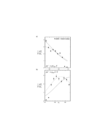
FIG. 19.: a) Comparison of our spectra $F(x_{L})$ for leading pions with data from Ref. [62] in the reaction $\pi^{+}+p\rightarrow\pi^{+}+p+X$. Solid and dashed lines correspond to the choices $m_{0}=0.35$ GeV and $m_{0}=0.45$ GeV respectively. b) the same as a) for the leading proton spectrum $F(x_{F})$ measured in the same reaction.

The EHS/NA22 collaboration provided us with data on $\pi^{+}+p\rightarrow\pi^{+}+p+X$ reactions. In particular they present the $x_{F}$ distributions of both leading particles, the pion and the proton. Their points for pions and protons are shown in Fig. 19a) and b) respectively. These points are presumably free from diffractive dissociation. The above mentioned asymmetry in pion and proton energy loss emerges clearly, the pions being much slower. The proton distribution peaks at $x_{F}\simeq 0.6-0.8$. Our curves (solid lines) reproduce with no free parameter this behaviour and we obtain a good agreement with the pion spectrum. Proton data show an excess at large $x_{F}$ that we are not able to reproduce keeping the same values of parameters as before.

The authors of Ref. [62] tried to fit their measured proton spectrum with the FRITIOF code and could not obtain a good description of data. This indicates that these large $x_{F}$ points are a problem for standard multiparticle production models as well. In our case, if we change our parameter $m_{0}$ from the usual value $m_{0}=0.35\,GeV$ (solid line) to $m_{0}=0.45\,GeV$ (dashed line) we can reproduce most of data points both for pions and protons as well. This is not a big change and indicates that the model would be able to accomodate this new experimental information. Of course, a definite statement about the subject would require a global refitting procedure, which is not our main concern now.

B Leading particles in photon-proton collisions

If, at high energies, the reactions $\rho-p$ and $\pi-p$ have the same characteristics and if VDM is a good hypothesis, then more about the energy flow in meson-$p$ collisions can be learned at HERA. Indeed, as mentioned in [54], at the HERA electron-proton collider the bulk of the cross section corresponds to photoproduction, in which a beam electron is scattered through a very small angle and a quasi-real photon interacts with the proton. Using VDM, high energy photoproduction exhibits therefore similar characteristics to hadron-hadron interactions.

Data taken by the ZEUS collaboration at HERA [63] show that the LP spectra measured in photoproducion and in DIS (where $Q^{2}\geq 4\,\,GeV^{2}$) are very similar, specially in the large $x_{L}$ region. This suggests that, as pointed out in [72], the QCD hardness scale for particle production in DIS gradually decreases from a (large) $Q^{2}$, which is relevant in the photon fragmentation region, to a soft scale in the proton fragmentation region, which is the one considered here. We can therefore expect a similarity of the inclusive spectra of the leading protons in high energy hadron-proton collisions, discussed above, and in virtual photon-proton collisions. In other words, we may say that the photon is neither resolving nor being resolved by the fast emerging protons. This implies that these reactions are dominated by some non-perturbative mechanism. This is confirmed by the failure of perturbative QCD [73], (implemented by the Monte Carlo codes ARIADNE and HERWIG) when applied to the proton fragmentation region. In Ref. [72] the LP spectra were studied in the context of meson and Pomeron exchanges. Here we use the vector meson dominance hypothesis and describe leading proton production in the same way as done for hadron-hadron collisions. The only change is that now we have $\rho-p$ instead of $p-p$ collisions. Whereas this may be generally true for photoproduction, it remains an approximation for DIS, valid in the large $x_{L}$ region.

Assuming that VDM is correct, the incoming photon line can be replaced by solid line in Fig. 1. During the interaction the photon is converted into a hadronic state, called $V$, and then interacts with the incoming proton. At HERA only collisions $V-p$ are relevant. The state $V$ looses fraction $x$ of its original momentum and gets excited carrying a $x_{F}=1-x$ fraction of the initial momentum. The proton, which we call here the diffracted proton, looses only a fraction $y$ of its momentum but otherwise remains intact. We assume here, for simplicity, that the vector meson is a $\rho^{0}$ and take $G^{\rho^{0}}(x)=G^{\pi}(x)$ in eqs. (7) and (9).

FIG. 20.: Comparison between our calculation and the data on the leading proton spectrum measured at HERA by the ZEUS Collab. [23].

In Fig. 20 we present our spectrum of leading protons in $\gamma p$ collisions. All parameters leading to the results in that figure are the same as established before in our study of diffractive mass distributions in photon-proton collision at HERA.

C Leading $J/\psi$ production

All produced particles come essentially from the gluons and quark-antiquark pairs already pre-existing in the projectile and target, or radiated during the collision. This qualitative picture takes different implementations in the many existing multiparticle production models. In the IGM, the produced particles (and consequently the energy released in the secondaries and lost by the projectiles) come almost entirely from the pre-existing gluons in the incoming hadrons. This conjecture may be directly tested using a high energy, nearly gluonless hadronic projectile. In this case, according to the IGM, inspite of the high energy involved, the production of secondaries would be suppressed in comparison to the production observed in reactions induced by ordinary hadrons. The energy would be mostly carried away by the projectile leading particle which would then be observed with a hard $x_{F}$ spectrum. This type of gluonless projectile is available in $J/\psi$ photoproduction, where the photon can be understood as a virtual $c\bar{c}$ pair which reacts with the proton and turns into the finally observed $J/\psi$. There are low energy data taken by the FTPS Collaboration [74] and high energy data from HERA [75].

We want to stress here the fact that the fair agreement with data observed in Figs. (18a) and (20) is possible only because the diffraction processes have been properly incorporated in the calculations. In other words, the inclusion of a diffractive component turns out to be a decisive factor to get agreement with data. We can also describe reasonably well pionic and kaonic LP and the observed difference turns out to be due to their different gluonic distributions.

FIG. 21.: Comparison of the IGM distribution $F(z)$ with data of Ref. [75] with restricted acceptance $p_{T}^{2}\geq 1\,(GeV/c)^{2}$ and $0.5\leq z\leq 0.9$ for fixed value of $\sigma^{inel}_{J/\psi-p}=9\,mb$ and for three different values of $p^{J/\psi}$: $0.066$ (dashed line), $0.033$ (solid line) and $0.016$ (dotted line).

The crucial role played by the parameter $p$ (see eq. (11)) representing the energy-momentum fraction of a given hadron allocated to gluons is best seen in Fig. 21 where we show the fit to data for leading $J/\psi$ photoproduction [75]. The only parameter to which results are really sensitive is $p=p^{J/\psi}$ which, as shown in Fig. 21, has to be very small, $p^{J/\psi}=0.033$. This is what could be expected from the fact that charmonium is a non-relativistic system and almost all its mass comes from the quark masses leaving therefore only a small fraction,

$$p^{J/\psi}\,=\,\frac{M_{J/\psi}-2m_{c}}{M_{J/\psi}}\,\simeq\,0.033,$$ (27)

for gluons (here $m_{c}=1.5\,GeV$ and $M_{J/\psi}=3.1\,GeV$). Of course, the value of $p^{J/\psi}$ required to give a very good fit of data might change either with another choice of $m_{c}$ or another choice of $\sigma^{inel}_{J/\psi-p}$. However these changes might affect $p^{J/\psi}$ by, at most, a factor two. This suggests that the momentum fraction carried by gluons in the $J/\psi$ is one order of magnitude smaller than that carried by gluons in light hadrons.

IX Summary and conclusions

We were able to fit an impressive amount of experimental data, which had nothing in common except the fact that they always referred to the momentum (or rapidity) distribution of some observed particle or to the invariant mass distribution of a cluster of measured particles. We could fit these data starting from one single ”generating” function, $\chi(x,y)$, which depends almost only on the density and interaction cross section of the gluons inside hadrons. These are fundamental quantities in QCD and with our model we can test the existing results for them. More than just fitting, we did some predictions and one of them, the leading particle spectrum shown in Fig. 20, was confirmed by experiment.

After all these works, we may ask ourselves what have we learned. We believe that we have constructed a simple and consistent picture of energy flow in strong interactions, based on the assumption that energy loss and leading particle spectra are determined by many independent gluon-gluon collisions and valence quarks play a secondary role. Consequently, energy flow will reflect the properties of the gluon distributions and cross sections in the colliding hadrons. This picture seems to be universal, i.e., valid in many different contexts. However, in order to see this universality we have to be careful and use proper kinematical limits of the phase space for every reaction considered, as illustrated in Figs. 1 and 2. When this is done the sensitivity of energy flow to other (than gluon distributions and cross sections) aspects of the production process is only of secondary importance and needs special observables (which are sensitive to, for example, the quantum numbers of the detected particles) to be visible. But even then, the IGM is indispensable because it provides the important energy correlations between different parts of the phase space.

Our analysis shows also clearly that our model can be regarded as a useful reference point for all more sophisticated approaches whereas, for hydrodynamical approaches of multiparticle production, it provides the initial energy used for the further evolution and hadronization of the created systems. However, in order to comply with the recent developments of QCD concerning the low $x$ gluonic content of hadrons [26, 27] it must be accordingly updated. We plan to do this in the future. We also plan to account for the intrinsic fluctuations present in the hadronizing systems. In the usual statistical models this can be done by using the so called nonextensive statistics and, as was shown in [76], it can influence substantially some energy flow results, in particular the estimation of inelasticity $K$.

A

The main ideas

The IGM can be summarized in the following way:

• The two colliding hadrons are represented by valence quarks carrying their quantum numbers plus the accompanying clouds of gluons.

• In the course of a collision the gluonic clouds interact strongly depositing in the central region of the reaction fractions $x$ and $y$ of the initial energy-momenta of the respective projectiles in the form of a gluonic Central Fireball (CF).

• The valence quarks get excited and form Leading Jets (LJ’s) which decay and populate mainly the fragmentation regions of the reaction.

The fraction of energy stored in the CF is therefore equal to $K\,=\,\sqrt{xy}$ and its rapidity is $Y=\frac{1}{2}\,\ln\frac{x}{y}$.

The CF consists of minifireballs (MF) formed from pairs of colliding gluons. In collisions at higher scales a MF is the same as a pair of minijets or jets. In the study of energy flow the details of fragmentation and hadron production are not important. Most of the MF’s will be in the central region and we assume that they coalesce forming the CF. The collisions leading to MF’s occur at different energy scales given by $Q^{2}_{i}=x_{i}\,y_{i}\,s$, where the index $i$ labels a particular kinematic configuration where the gluon from the projectile has momentum $x_{i}$ and the gluon from the target has $y_{i}$. We have to choose the scale where we start to use perturbative QCD. Below this value we have to assume that we can still talk about individual soft gluons and due to the short correlation length between them they still interact mostly pairwise. In this region we can no longer use the distribution functions extracted from DIS nor the perturbative elementary cross sections.

The central formula

The central quantity in the IGM is the probability to form a CF carrying momentum fractions $x$ and $y$ of two colliding hadrons. It is defined as the sum over an undefined number n of MF’s:

$$\chi(x,y) = \sum_{n_{1}}\,\sum_{n_{2}}\cdots\sum_{n_{i}}\,\delta\left[x-n_{1}\,x_{1}-\cdots-n_{i}\,x_{i}\right]$$ (A1)

$$\times \,\delta\left[y-n_{1}\,y_{1}-\cdots-n_{i}\,y_{i}\right]\,P(n_{1})\cdots P(n_{i})$$ (A2)

$$= \sum_{\{n_{i}\}}\left\{\delta\left[x-\sum_{i}n_{i}\,x_{i}\right]\delta\left[y-\sum_{i}n_{i}\,y_{i}\right]\right\}$$ (A3)

$$\times \prod_{\{n_{i}\}}P(n_{i})$$ (A4)

The delta functions in the above formula garantee energy momentum conservation and $P(n_{i})$ is the probability to have $n_{i}$ collisions between gluons with $x_{i}$ and $y_{i}$. The expression above is quite general. It becomes specific when we define $P(n_{i})$. The assumption of multiple parton-parton incoherent scattering (which is also used in Refs. [1, 29, 30, 31, 34]) implies a Poissonian distribution of the number of parton-parton collisions and thus $P(n_{i})$ is given by:

$$P(n_{i}) = \frac{(\overline{n}_{i})^{n_{i}}\,exp(-\overline{n}_{i})}{n_{i}\,!}$$ (A5)

Inserting $P(n_{i})$ in (A4) and using the following integral representations for the delta functions:

$$\delta\left[x-\sum_{i}n_{i}\,x_{i}\right]\,=$$ (A6)

$$= \frac{1}{2\pi}\int^{+\infty}_{-\infty}dt\,\exp\left[it\left(x-\sum_{i}n_{i}\,x_{i}\right)\right]$$ (A7)

$$\delta\left[y-\sum_{i}n_{i}\,y_{i}\right]\,=$$ (A8)

$$= \frac{1}{2\pi}\int^{+\infty}_{-\infty}du\,\exp\left[iu\left(y-\sum_{i}n_{i}\,y_{i}\right)\right]$$ (A9)

we can perform all summations and products arriving at:

$$\chi(x,y)\, = \,\frac{1}{(2\pi)^{2}}\int^{+\infty}_{-\infty}dt\int^{+\infty}_{-\infty}du\,\exp\,[i(tx+uy)]$$ (A10)

$$\times \exp\left\{\sum_{i}\left\{\overline{n}_{i}\left[e^{-i(tx_{i}+uy_{i})}-1\right]\right\}\right\}$$ (A11)

Taking now the continuum limit:

$$\overline{n}_{i}\,=\,\frac{d\overline{n}_{i}}{dx^{\prime}\,dy^{\prime}}\,\Delta x^{\prime}\Delta y^{\prime}\;\;\longrightarrow\;\;d\overline{n}\,=\,\frac{d\overline{n}}{dx^{\prime}\,dy^{\prime}}\,dx^{\prime}\,dy^{\prime}$$ (A12)

we obtain:

$$\chi(x,y)=\frac{1}{(2\pi)^{2}}\int^{+\infty}_{-\infty}dt\int^{+\infty}_{-\infty}du\,\exp[i(tx+uy)]$$ (A13)

$$\times \exp\left\{\int^{1}_{0}dx^{\prime}\int^{1}_{0}dy^{\prime}\,\omega(x^{\prime},y^{\prime})\left[e^{-i(tx^{\prime}+uy^{\prime})}-1\right]\right\}$$ (A14)

where

$$\omega(x^{\prime},y^{\prime})\,=\,\frac{d\overline{n}}{dx^{\prime}\,dy^{\prime}}.$$ (A15)

This function $\omega(x^{\prime},y^{\prime})$ is called the spectral function and represents the average number of gluon-gluon collisions as a function of $x^{\prime}$ e $y^{\prime}$. It contains all the dynamical inputs of the model and has the form:

$$\omega(x^{\prime},y^{\prime})\, = \,\frac{\sigma_{gg}(x^{\prime}y^{\prime}s)}{\sigma(s)}\,G(x^{\prime})\,G(y^{\prime})$$ (A16)

$$\times \theta\left(x^{\prime}y^{\prime}-K^{2}_{min}\right),$$ (A17)

where $G$’s denote the gluon distribution functions in the corresponding projectiles and $\sigma_{gg}$ and $\sigma$ are the gluon-gluon and hadron-hadron cross sections, respectively. In the above expression $x^{\prime}$ and $y^{\prime}$ are the fractional momenta of two gluons coming from the projectile and from the target whereas $K_{min}=m_{0}/\sqrt{s}$, with $m_{0}$ being the mass of lightest produced state and $\sqrt{s}$ the total c.m.s. energy. $m_{0}$ is a parameter of the model.

The integral in the second line of eq. (A14) is dominated by the low $x^{\prime}$ and $y^{\prime}$ region. Considering the singular behavior of the $G(x)$ distributions at the origin we make the following approximation:

$$e^{-i(tx^{\prime}+uy^{\prime})}-1\,\simeq\,-i(tx^{\prime}+uy^{\prime})-\frac{1}{2}(tx^{\prime}+uy^{\prime})^{2}$$ (A18)

With this approximation it is possible to perform the integrations in (A14) and obtain the final expression for $\chi(x,y)$ discussed in the main text:

$$\chi(x,y)=\frac{\chi_{0}}{2\pi\sqrt{D_{xy}}}\,\exp\{-\frac{1}{2D_{xy}}[\langle y^{2}\rangle(x-\langle x\rangle)^{2}$$ (A19)

$$+ \,\langle x^{2}\rangle(y-\langle y\rangle)^{2}+\,2\,\langle xy\rangle(x-\langle x\rangle)\,(y-\langle y\rangle)]\}$$ (A20)

where

$$D_{xy} = \langle x^{2}\rangle\langle y^{2}\rangle-\langle xy\rangle^{2}$$ (A21)

and

$$\langle x^{n}y^{m}\rangle = \int_{0}^{1}\!dx\,x^{n}\,\int_{0}^{1}\!dy\,y^{m}\,\omega(x,y),$$ (A22)

$\chi_{0}$ is a normalization factor defined by the condition:

$$\int_{0}^{1}\!dx\,\int_{0}^{1}\!dy\,\chi(x,y)\theta(xy-K_{min}^{2})=1$$ (A23)

The numerical inputs

In order to evaluate the distribution (A20) we need to choose the value of $m_{0}$, the semihard scale $p_{T\,min}$ and define $G(x)$ and $\sigma_{gg}$ in both interaction regimes. We take $p_{T\,min}\,=\,2.3\,GeV$ and $m_{0}\,=\,0.35\,GeV$. These are the two scales present in the model. The semihard gluon-gluon cross section is taken, at order $\alpha_{s}^{2}$, to be:

$$\hat{\sigma}^{h}_{gg}(x\,,\,y\,,\,s)\,=\,\kappa\frac{\pi}{16\,p^{2}_{T\,min}}\left[\alpha_{s}(Q^{2})\right]^{2}\,H$$ (A24)

where

$$H=36T\,+\frac{51\lambda T}{4\,x\,y}-\frac{3\lambda^{2}\,T}{8\,x^{2}\,y^{2}}+\frac{9\lambda}{x\,y}\,\ln\left[\,\frac{1-T}{1+T}\,\right]$$ (A25)

and

$$T\,=\,\left[1-\frac{\lambda}{x\,y}\right]^{\frac{1}{2}}\,;\,\lambda\,=\,\frac{4\,p^{2}_{T\,min}}{s}$$ (A26)

The parameter $\kappa$ is the one frequently used to incorporate higher corrections in $\alpha_{s}$ and is $1.1\leq\kappa\leq 2.5$ according to the choice of $G(x)$, of the scale $Q^{2}$ and $p_{T\,min}$. For $p_{T\,min}=2.3\,GeV$, $\kappa=2.5$.

The coupling constant is given by:

$$\alpha_{s}(Q^{2})\,=\,\frac{12\,\pi}{\left(33-2N_{f}\right)\,\ln\left[\frac{Q^{2}}{\Lambda^{2}}\right]}$$ (A27)

where $\Lambda\,=\,0.2\,GeV$ and $N_{f}\,=\,3$ is the number of active flavors. As usual in minijet physics we choose $Q^{2}\,=\,p^{2}_{T\,min}$ and use the distributions $G(x,Q^{2})$ parametrized in literature.

When the invariant energy of the gluon pair $\hat{s}$ is the interval $m^{2}_{0}\,\leq\,\hat{s}\,=\,xys\,\leq\,4p^{2}_{T\,min}$ we are outside the perturbative domain. Parton-parton cross sections in the non-perturbative regime have been parametrized in [77] leading to a successful quark-gluon model for elastic and diffractive scattering. Recently these non-perturbative cross sections have been calculated in the stochastic vacuum model [78]. The obtained cross sections are functions of the gluon condensate and of the gluon field correlation length, both quantities extracted from lattice QCD calculations. In order to keep our treatment simple we adopt the older parametrization for the gluon-gluon cross section used in [77]:

$$\hat{\sigma}^{s}_{gg}(x\,,\,y\,,\,s)\,=\,\frac{\alpha}{x\,y\,s}$$ (A28)

where $\alpha$ is a parameter of the model [11].

The main distributions

Given $\chi(x,y)$ we can immediately write the inelasticity distribution, its complementary distribution, the leading jet momentum spectrum and the CF rapidity distribution:

$$\chi(K) = \int^{1}_{0}dx\int^{1}_{0}dy\,\chi(x,y)\,\delta\left(\sqrt{xy}-K\right)$$ (A29)

$$\times \,\theta\left(xy-K^{2}_{min}\right)$$ (A30)

$$F(x_{L})\,=\, (1-\alpha)\int^{1}_{x_{min}}\!\!dx\,\chi^{(nd)}\left(x;y=1-x_{L}\right)\,+$$ (A32)

$$+\,\sum_{j=1,2}\alpha_{j}\int^{1}_{x_{min}}\!\!dx\,\chi^{(d)}\left(x;y=1-x_{L}\right)$$

$$\chi(Y) = \int^{1}_{0}dx\int^{1}_{0}dy\,\chi(x,y)\,\delta\left(\frac{1}{2}\,ln\,\left(\frac{x}{y}\right)-Y\right)$$ (A33)

$$\times \,\theta\left(xy-K^{2}_{min}\right)$$ (A34)

where $\alpha=\alpha_{1}+\alpha_{2}$ is the total fraction of single diffractive $(d)$ events (from the upper and lower legs in Fig. 1, respectively) and where

$$x_{min}={\rm Max}\left[\frac{m_{0}^{2}}{(1-x_{L})s};\frac{\left(M_{LP}+m_{0})\right)^{2}}{s}\right]$$ (A35)

The mass spectra for Single Diffractive processes are given by:

$$\frac{1}{\sigma}\frac{d\sigma}{dM_{X}^{2}} = \frac{dN}{dM_{X}^{2}}=\int_{0}^{1}dx\,\int_{0}^{1}dy\,\chi(x,y)$$ (A36)

$$\times \,\delta\left(M^{2}_{X}-sy\right)\,\theta\left(xy-K_{min}^{2}\right)$$ (A37)

Substituting now eq. (A20) into eq. (A37) we arrive at the following simple expression for the diffractive mass distribution:

$$\frac{dN}{dM^{2}_{X}}\,=\,\frac{1}{s}\,F(M^{2}_{X},s)\,H(M_{X}^{2},s)$$ (A38)

where

$$F(M^{2}_{X},s) = \exp\left[-\frac{\langle x^{2}\rangle}{2D_{xy}}\,\left(\frac{M^{2}_{X}}{s}-\langle y\rangle\right)^{2}\right]$$ (A39)

and

$$H(M^{2}_{X},s)=\frac{\chi_{0}}{2\pi\sqrt{D_{xy}}}\,\int^{1}_{\!{}_{\frac{m_{0}^{2}}{M_{X}^{2}}}}\!dx\,\exp\left\{-\frac{1}{2D_{xy}}\,Z\right\},$$ (A40)

$$Z=[\langle y^{2}\rangle(x-\langle x\rangle)^{2}-2\langle xy\rangle(x-\langle x\rangle)(M_{X}^{2}/s-\langle y\rangle)]$$

We first keep only the most singular parts of the gluonic distributions used (i.e., $G(x)\simeq 1/x$) and collect all other factors in eq. (A17) in a single parameter $c$. Assuming that the ratio of the cross sections $\frac{\sigma(xys)}{\sigma(s)}$ does not depend on $x$ and $y$ and neglecting all terms of the order of $\frac{m_{0}^{2}}{s}$ and $\frac{m_{0}^{2}}{M_{X}^{2}}$, we arrive at the following expressions for the moments calculated in eq. (A22):

$$\langle x\rangle\, = 2\,\langle x^{2}\rangle\simeq\,c\,\ln\frac{M_{X}^{2}}{m_{0}^{2}}$$ (A41)

$$\langle y\rangle\, = 2\,\frac{s}{M_{X}^{2}}\,\langle y^{2}\rangle\simeq\,c\,\frac{M_{X}^{2}}{s}\,\ln\frac{M_{X}^{2}}{m_{0}^{2}}$$ (A42)

$$\langle x\,y\rangle\, \simeq \,c\,\left(\frac{M_{X}^{2}}{s}\,-\frac{m_{0}^{2}}{s}\,\ln\frac{M_{X}^{2}}{m_{0}^{2}}\right)$$ (A43)

Notice that in all cases of interest $\langle x\,y\rangle$ is much smaller than other moments (by a factor $\ln\frac{M_{X}^{2}}{m_{0}^{2}}$, at least). It means that $D_{xy}\,\simeq\,\langle x^{2}\rangle\langle y^{2}\rangle$ and consequently

$$F(M^{2}_{X},s)\, \simeq \,\exp\left[-\frac{\left(\frac{M_{X}^{2}}{s}\,-\,\langle y\rangle\right)^{2}}{2\,\langle y^{2}\rangle}\right]$$ (A44)

$$\simeq \,\exp\left[-\frac{\left(1\,-\,c\,\ln\frac{M_{X}^{2}}{m_{0}^{2}}\right)^{2}}{c\,\ln\frac{M_{X}^{2}}{m_{0}^{2}}}\right]$$ (A45)

and

$$H(M_{X}^{2},s)\, \simeq \,\frac{\chi_{0}}{2\pi\sqrt{D_{xy}}}\,\int^{1}_{\!{}_{\frac{m_{0}^{2}}{M_{X}^{2}}}}\!dx\exp\left[-\frac{(x-\langle x\rangle)^{2}}{2\langle x^{2}\rangle}\right]$$ (A46)

$$\simeq \,{\rm const}\,\frac{\sqrt{\langle x^{2}\rangle}}{\sqrt{D_{xy}}}\,=\,{\rm const}\,\frac{1}{\sqrt{\langle y^{2}\rangle}}$$ (A47)

$$\simeq \,{\rm const}\,\frac{s}{M_{X}^{2}\,\sqrt{c\,\ln\frac{M_{X}^{2}}{m_{0}^{2}}}}$$ (A48)

leading to

$$\frac{dN}{dM_{X}^{2}}\, \simeq \,\frac{1}{s}\,H(M_{X}^{2},s)\,F(M^{2}_{X},s)\simeq\,\frac{\rm const}{M_{X}^{2}}\,\times$$ (A49)

$$\times \frac{1}{\sqrt{c\,\ln\frac{M_{X}^{2}}{m_{0}^{2}}}}\,\exp\left[-\frac{\left(1\,-\,c\,\ln\frac{M_{X}^{2}}{m_{0}^{2}}\right)^{2}}{c\,\ln\frac{M_{X}^{2}}{m_{0}^{2}}}\right]$$ (A50)

The mass spectra for Double Pomeron Exchange processes are given by:

$$\frac{1}{\sigma}\frac{d\sigma}{dM_{XY}} = \frac{dN}{dM_{XY}}=\int_{0}^{1}dx\,\int_{0}^{1}dy\,\chi(x,y)$$ (A51)

$$\times \,\delta\left(M_{XY}-\sqrt{xys}\right)\,\theta\left(xy-K_{min}^{2}\right)$$ (A52)

B

The ”kinematical” Pomeron

The Pomeron for us is just a collection of gluons which belong to the diffracted proton or antiproton. These gluons behave like all other ordinary gluons in the proton and have therefore the same momentum distribution. The only difference is the momentum sum rule, which for the gluons in $I\!\!P$ is:

$$\int_{0}^{1}\!dx^{\prime}\,x^{\prime}\,G_{I\!\!P}(x^{\prime})\,=\,p_{d}$$ (B1)

where $p_{d}=0.05$ (see [15]) instead of $p=0.5$, which holds for the entire gluon population in the proton.

In order to make contact with the analysis performed by HERA experimental groups we consider two possible momentum distributions for the gluons inside $I\!\!P$. A hard one:

$$f^{h}_{g/I\!\!P}(\beta) = a_{h}\,(1\,-\,\beta)$$ (B2)

and a “super-hard” (or “leading gluon”) one:

$$f^{sh}_{g/I\!\!P}(\beta) = a_{sh}\,\beta^{7}\,(1\,-\,\beta)^{0.3}$$ (B3)

where $\beta$ is the momentum fraction of the Pomeron carried by the gluons and the superscripts $h$ and $sh$ denote hard and superhard respectively. The constants $a_{h}$ and $a_{sh}$ will be fixed by the sum rule (B1). In the past, following the same formalism, we have also considered a soft gluon distribution for the Pomeron of the type

$$f^{s}_{g/I\!\!P}(\beta)=6\,\frac{(1\,-\,\beta)^{5}}{\beta}$$ (B4)

but we found that this “soft Pomeron” distribution was incompatible with the single diffractive mass spectra measured at HERA [79]. This Pomeron profile was also ruled out by other types of observables, as concluded in Refs. [80] and [54].

We use the Donnachie-Landshoff Pomeron flux factor, which, after the integration in the $t$ variable, is approximately given by [58]:

$$f_{I\!\!P/p}(x_{I\!\!P})\simeq C\,x_{I\!\!P}^{1-2\alpha_{I\!\!P}}\simeq C\,\frac{1}{x_{I\!\!P}}$$ (B5)

where $x_{I\!\!P}$ is the fraction of the proton momentum carried by the Pomeron and the normalization constant $C$ fixed also with the help of (B1). Noticing that $\beta=\frac{x}{x_{I\!\!P}}$, the distribution $G_{I\!\!P}(y)$ needed in eqs. (7) and (9) is then given by the convolution:

$$G^{s,h,sh}_{I\!\!P}(y) = \int_{y}^{1}\!\frac{dx_{I\!\!P}}{x_{I\!\!P}}\,f_{I\!\!P/p}(x_{I\!\!P})\,f^{s,h,sh}_{g/I\!\!P}(\frac{y}{x_{I\!\!P}})$$ (B6)

We use also the “diffractive gluon distribution” given by:

$$G_{I\!\!P}(y)=a\,\frac{(1\,-\,y)^{5}}{y}$$ (B7)

where $a$ is fixed by the sum rule.

Acknowledgements: This work has been supported by FAPESP, CNPQ (Brazil) (FOD and FSN) and by KBN (Poland) (GW). We are indebted to our colleagues Y. Hama, T. Kodama, M. Menon, F. Grassi, S. Padula, members of the “Projeto Temático FAPESP” and also to R. Covolan and A. Natale, V.P Gonçalves for fruitful discussions.

REFERENCES

- [1] X. N. Wang and M. Gyulassy, Phys. Rev. D44, 3501 (1991); D45, 844 (1992).
- [2] K. Werner, Phys. Rept. 232, 87 (1993).
- [3] H.J. Drescher, M. Hladik, S. Ostapchenko, T. Pierog and K. Werner, Phys. Rept. 350, 93 (2001).
- [4] K.J. Eskola, Nucl. Phys. A698, 78 (2002); S.A. Bass et al., Prog. Part. Nucl. 41, 225 (1998).
- [5] W. Heisenberg, Z.Phys. 126, 569 (1949); E. Fermi, Prog. Theor. Phys. 5, 570 (1950); I. Pomeranchuk, Dokl. Akad. Nauk SSSR 78, 889 (1951); L.D. Landau and S.Z. Bilenkij, Nuovo Cim. Suppl. 3, 15 (1956); R. Hagedorn, Riv. Nuovo Cim. 3, 147 (1965); Nuovo Cim. A52, 64 (1067); Riv. Nuovo Cim. 6, 1 (1983).
- [6] F. Beccatini and L. Ferroni, Eur. Phys. J. C35, 243 (2004); hep-ph/0407117 and references therein.
- [7] E.M. Friedlander et al., Mod. Phys. Lett. A3, 1461 (1988).
- [8] Cf. Proceedings of QM2004, J. Phys. G30, 8 (2004) and references therein.
- [9] Yu.M. Shabelski, R.M. Weiner, G. Wilk and Z. Włodarczyk, J. Phys. G18, 1281 (1992) and references therein; A.A. Watson, Nucl. Phys. B (Proc. Suppl.) 60, 171 (1998).
- [10] S. Pokorski and L. Van Hove, Acta Phys. Polon. B5, 229 (1974) and Nucl. Phys. B86, 243 (1975); G.N. Fowler, R.M. Weiner and G. Wilk, Phys. Rev. Lett. 55, 173 (1985).
- [11] G.N. Fowler, F.S. Navarra, M. Plümer, A. Vourdas, R.M. Weiner and G. Wilk, Phys. Lett. B214, 657 (1988) and Phys. Rev. C40, 1219 (1989).
- [12] F.O. Durães, F.S. Navarra and G Wilk, Phys. Rev. D47, 3049 (1993).
- [13] F.O. Durães, F.S. Navarra and G Wilk, Phys. Rev. D50, 6804 (1994).
- [14] F.O. Durães, F.S. Navarra, C.A.A. Nunes and G. Wilk, Phys. Rev. D53, 6136 (1996).
- [15] F.O. Durães, F.S. Navarra and G Wilk, Phys. Rev. D55, 2708 (1997).
- [16] F.O. Durães, F.S. Navarra and G Wilk, Phys. Rev. D56, R2499 (1997).
- [17] F.O. Durães, F.S. Navarra and G Wilk, Phys. Rev. D58, 094034 (1998).
- [18] F.O. Durães, F.S. Navarra and G Wilk, Mod. Phys. Lett. A13, 2873 (1998).
- [19] F.O. Durães, F.S. Navarra and G Wilk, Braz. Jour. Phys. 28, 505 (1998).
- [20] S. Paiva, Y. Hama and T. Kodama, Phys. Rev. C55, 1455 (1997); S. Paiva and Y. Hama, Phys. Rev. Lett. 78, 3070 (1997).
- [21] J. Bellandi, R.J.M. Covolan and A.L. Godoi, Phys. Lett. B343, 410 (1995).
- [22] J. Bellandi, R.J.M. Covolan, A.L. Godoi and J. Montanha, J. Phys. G23, 125 (1997).
- [23] M. Arneodo et al., (ZEUS Collab.), Nucl. Phys. B658, 3 (2003).
- [24] A. Brandt et al., (UA8 Collab.), Eur. Phys. Jour. C25, 361 (2002).
- [25] F.O. Durães, F.S. Navarra and G Wilk, Phys. Rev. D67, 074002 (2003).
- [26] For recent reviews see: E. Iancu, A. Leonidov and L. McLerran, The Colour Glass Condensate: An Introduction, hep-ph/0202270, published in QCD Perspectives on Hot and Dense Matter, Eds. J.-P. Blaizot and E. Iancu, NATO Science Series, Kluwer, 2002; E. Iancu and R. Venugopalan, T͡he Color Glass Condensate and High Energy Scattering in QCD, hep-ph/0303204.
- [27] A. Dumitru, L. Gerland and M. Strikman, Phys. Rev.Lett. 90, 092301 (2003); Erratum-ibid. 91, 259901 (2003).
- [28] T.K. Gaisser and F. Halzen, Phys. Rev. Lett. 54, 1754 (1985); F.S. Navarra and D. Treleani, Int. J. Mod. Phys. E2, 207 (1993).
- [29] N. Brown, Mod. Phys. Lett. A4, 2447 (1989).
- [30] T.K. Gaisser and T. Stanev, Phys. Lett. B219, 375 (1989).
- [31] T. Sjostrand and M. van Zijl, Phys. Rev. D36, 2019 (1987).
- [32] K.Geiger, Phys. Rev. D46, 4965 (1992); 46, 4986 (1992).
- [33] S. Lupia, W. Ochs and J. Wosiek, Nucl. Phys. B540, 405 (1999).
- [34] S. Sapeta, Phys. Lett. B597, 352 (2004).
- [35] A. di Giacomo and H. Panagopoulos, Phys. Lett. B285, 133 (1992).
- [36] T. Schaefer and E. Shuryak, Rev. Mod. Phys. 70, 323 (1998).
- [37] E. Shuryak, Phys. Lett. B486, 378 (2000).
- [38] J. Pumplin et al., JHEP 0207, 012 (2002).
- [39] A.D. Martin, R.G. Roberts, W.J. Stirling and R.S. Thorne, hep-ph/0411040, hep-ph/0407311 and references therein.
- [40] M. Glück, C. Pisano and E. Reya, hep-ph/0412049; M. Glück and E. Reya, hep-ph/0203063 and references therein.
- [41] M. Glück, E. Reya and A. Vogt, Z. Phys. C47, 433 (1995).
- [42] D. Diakonov, hep-ph/0406043 and references therein; F.S. Navarra, Marina Nielsen, M.R. Robilotta, J. Phys. G19, 685 (1993).
- [43] D. Diakonov, V. Petrov and P.V. Pobylitsa, Nucl. Phys. B306, 809 (1988).
- [44] R. Luna, A. Zepeda, C.A. Garcia Canal, S.J. Sciutto, hep-ph/0408303
- [45] C. Geich-Gimbel, Int. Jour. Mod. Phys. A4, 1527 (1989).
- [46] F. Abe et al., Phys. Rev. D41, 2330 (1990).
- [47] M. Adamovich et al., (WA82 Collab.), Phys. Lett. B306, 402 (1993); G.A. Alves et al., (E769 Collab.), Phys. Rev. Lett. 72, 812 (1994); E.M. Aitala et al., (E791 Collab.), Phys. Lett. B371, 157 (1996).
- [48] S. Frixione et al., Nucl. Phys. B431, 453 (1994); P. Nason, S. Dawson and K.Ellis, Nucl. Phys. B327, 49 (1989).
- [49] T. Sjöstrand, Comp. Phys. Commun. 39, 344 (1986); T. Sjöstrand and Bengtsson, Comp. Phys. Commun. 43, 367 (1987).
- [50] H. Forkel et al., Phys. Rev. C50, 3108 (1994); F. Carvalho et al., Phys. Rev. Lett. 86, 5434 (2001).
- [51] N.A. Amos et al., (E710 Collab.), Phys. Lett. B301, 313 (1993); F. Abe et al., (CDF Collab.), Phys. Rev. D50, 5535 (1994).
- [52] M.G. Albrow et at., Nucl. Phys. B108, 1 (1976).
- [53] N.A. Amos et al., (E710 Collab.), Phys. Lett. B301, 313 (1993); F. Abe et al., (CDF Collab.), Phys. Rev. D50, 5535 (1994).
- [54] C. Adloff et al., (H1 Collab.), Z. Phys. C74, 221 (1997).
- [55] J.C. Collins, L. Frankfurt and M. Strikman, Phys. Lett. B307, 161 (1993).
- [56] A. Berera and D.E. Soper. Phys. Rev. D53, 6162 (1996).
- [57] A. Berera and J.C. Collins, Nucl. Phys. B474, 183 (1996).
- [58] L. Alvero, J.C. Collins, J. Terron and J.J. Witmore, Phys. Rev. D59, 074022 (1999).
- [59] A. Berera, Phys. Rev. D62, 014015 (2000).
- [60] A.E. Brenner et al., Phys. Rev. D26, 1497 (1982).
- [61] D.S. Barton et al., Phys. Rev. D27, 2580 (1983).
- [62] N.M. Agababyan et al., (EHS/NA22 Collab.), Z. Phys. C75, 229 (1996).
- [63] N. Cartiglia, Leading Baryons at Low in DIS and Photoproduction at ZEUS, hep-ph/9706416.
- [64] S.D. Holmes, W. Lee and J.E. Wiss, Ann. Rev. Nucl. Part. Sci. 35, 397 (1985); T.H. Bauer, R.D. Spital, D.R. Yennie and F.M. Pipkin, Rev. Mod. Phys. 50, 261 (1978).
- [65] G.M. Frichter, T.K. Gaisser and T. Stanev, Phys. Rev. D56, 3135 (1997).
- [66] Cf., for example, A.A. Watson, Nucl. Phys. B (Proc. Suppl.) B60, 171 (1998); J.W. Cronin, Nucl. Phys. B (Proc. Suppl.) B28, 213 (1992); The Pierre Auger Project, Design Report, http://www-td-auger.fnal.gov
- [67] A. Berera et al., Phys. Lett. B403, 1 (1997).
- [68] W.D. Walker, Phys. Rev. D53, 1886 (1996).
- [69] G. Donaldson et al., Phys. Lett. B73, 375 (1978).
- [70] E. Fishbach and G.W. Look, Phys. Rev. D15, 2576 (1977).
- [71] D. Kharzeev, Phys. Lett. B378, 238 (1996); S.E.Vance, M.Gyulassy and X.-N. Wang, Phys. Lett. B443, 45 (1998) and references therein.
- [72] A. Szczurek, N.N. Nikolaev and J. Speth, Phys. Lett. B428, 383 (1998).
- [73] M. Derrick et al., (ZEUS Collab.), Phys. Lett. B384, 388 (1996).
- [74] B.H. Denby et al., Phys. Rev. Lett. 52, 795 (1984).
- [75] S. Aid et al., (H1 Collab.), Nucl. Phys. B472, 3 (1996); M. Derrick et al., (ZEUS Collab.), Phys. Lett. B350, 120 (1995); J. Breitweg et al., (ZEUS Collab.), Z. Phys. C76, 599 (1997).
- [76] F.S. Navarra, O.V. Utyuzh, G.Wilk and Z. Włodarczyk, Nuovo Cim. C24, 725 (2001); Phys. Rev. D67, 114002 (2003); Physica 340, 467 (2004); Physica 344, 568 (2004); Nukleonika 49, S19 (2004).
- [77] P. L’Hereux, B. Margolis and P. Valin, Phys. Rev. D32, 1 (1985).
- [78] A.F. Martini, M.J. Menon and D.S. Thober, Phys. Rev. D57, 3026 (1998).
- [79] T. Ahmed et al., (H1 Collab.), Nucl. Phys. B435, 3 (1995); B429, 477 (1994).
- [80] M. Derrick et al., (ZEUS Collab.), Phys. Lett. B356, 129 (1995); Z. Phys. C68, 569 (1995) and references therein.