New Source of CP violation in $B$ physics ?

In this talk we discuss how the down type left-right squark mixing in Supersymmetry can induce a new source of CP violation in the time dependent asymmtries in $B\to\phi K$ process. We use QCD improved factorization process to calculate the hadronic matrix element for the process and find the allowed parameter space for $\rho$ and $\phi$, the magnitude and phase of the down type LR(RL) squark mixing parameter $\delta^{bs}_{LR(RL)}$. In the same allowed regin we calculate the expected CP asymmtries in the $B\to\phi K^{*}$ process.

1 Introduction

Time dependent asymmetries measured in the decay $B\to\phi K_{S}$ both by BaBar and Belle collaborations [1, 2, 3, 4] show significant deviation from the standard model and this has generated much theoretical speculation regarding physics beyond the standard model [References-References]. In the standard model, the process $B\to\phi K_{S}$ is purely penguin dominated and the leading contribution has no weak phase. The coefficient of $\sin(\Delta m_{B}t)$ in the asymmetry therefore should measure $\sin 2\beta$, the same quantity that is involved in $B\to\psi K_{S}$ in the standard model. The most recent measured average values of asymmetries are  [4, 22]

$$S_{\psi K_{S}} = 0.734\pm 0.055$$

$$S_{\phi K_{S}} = -0.15\pm 0.33$$ (1)

The value for $S_{\psi K_{S}}$ agrees with theoretical expectation from the CKM matrix of $S_{\psi K_{S}}=\sin 2\beta=0.715^{+0.05}_{-0.045}$  [23]. This leads to the conclusion that CP phase in $B-\bar{B}$ mixing is consistent with the standard model. The deviation in the $\phi K_{S}$ is intriguing because a penguin process being a loop induced process is particularly sensitive to new physics which can manifest itself in a loop diagram through exchange of heavy particles. In this talk [24] we consider effects arising from non universal squark mixing in the second and third generation of the down type squarks in supersymmetric theory as the origin of additional contributions to the amplitude within the mass insertion approximation scheme. In particular, the exchanges of gluinos $(\tilde{g})$ and squark $(\tilde{q})$ with left-right mixing can enhance the Wilson coefficient of the gluonic dipole penguin operator ${\cal O}_{8g}$ by a factor of $m_{\tilde{g}}/m_{b}$ compared with the standard model prediction and we take into account its effect on the process $B\to\phi K_{S}$. In our analysis we take the $B-\bar{B}$ mixing phase the same as in the standard model as required by $\psi K_{S}$ data, and permitted in SUSY by requiring that the first and third generation squark mixing to be small. We study $B\to\phi K$ in QCD improved factorization scheme (BBNS approach ) [25]. This method incorporates elements of naive factorization approach (as its leading term ) and perturbative QCD corrections (as sub-leading contributions) and allows one to compute systematic radiative corrections to the naive factorization for the hadronic $B$ decays.

In supersymmetry, assuming masses of squarks $(\tilde{q})$ and gluinos $(\tilde{g})$, the new source of CP violation can be parameterized by the complex quantity $\delta^{bs}_{LR(RL)}$ written in the form $\rho e^{i\psi}$ We identify the region in $\rho-\psi$ plane allowed by the experimental data on $B\to\phi K$ time dependent asymmetries $S_{\phi K_{S}}$ and $C_{\phi K_{S}}$ and the branching ratio. This allowed region is dependent of the QCD scale $\mu$, therefore we illustrate the region for two values of $\mu=m_{b}$ and $m_{b}/2$. The same contribution should also be present in other penguin mediated process. We study the effect of $LR(RL)$ mass insertion to the $B\to\phi K^{\ast}$ decay mode which is also a pure penguin process using QCD improved factorization method. We then estimate the branching ratio ${\cal B}(B\to\phi K^{\ast})$ and the CP asymmetry ${\cal A}_{CP}$ in the parameter space of $\delta^{bs}_{LR(RL)}$ allowed by $B\to\phi K$ data. In this vector vector final state, one can also construct more CP violating observables [26]. We compute these observables in the same range of parameter space as that allowed by $B\to\phi K$.

2 CP Asymmetry of $B\to\phi K$

The time dependent CP asymmetry of $B\to\phi K_{S}$ is described by :

$${\cal A}_{\phi K_{S}}(t) = \frac{\Gamma(\overline{B^{0}}(t)\to\phi K_{S})-\Gamma(B^{0}(t)\to\phi K_{S})}{\Gamma(\overline{B^{0}}(t)\to\phi K_{S})+\Gamma(B^{0}(t)\to\phi K_{S})}$$ (2)

$$= -C_{\phi K_{S}}\cos(\Delta m_{B}t)+S_{\phi K}\sin(\Delta m_{B}t)$$ (3)

where $S_{\phi K}$ and $C_{\phi K_{S}}$ are given by

$$S_{\phi K}=\frac{2Im~{}\lambda_{\phi K_{S}}}{1+\mid\lambda_{\phi K_{S}}\mid^{2}},~{}~{}~{}~{}C_{\phi K_{S}}=\frac{1-\mid\lambda_{\phi K_{S}}\mid^{2}}{1+\mid\lambda_{\phi K_{S}}\mid^{2}}$$ (4)

and $\lambda_{\phi K_{S}}$ can be expressed in terms of decay amplitudes:

$$\lambda_{\phi K_{S}}=-e^{-2i\beta}\frac{{\overline{\cal M}}(\overline{B^{0}}\to\phi K_{S})}{{\cal M}(B^{0}\to\phi K_{S})}$$ (5)

The branching ratio and the direct CP asymmetries of both the charged and neutral modes of $B\to\phi K$ have been measured [1, 2, 3, 4, 22, 27]:

$${\cal B}(B^{0}\to\phi K_{S}) = (8.0\pm 1.3)\times 10^{-6}$$ (6)

$${\cal B}(B^{+}\to\phi K^{+}) = (9.4\pm 0.9)\times 10^{-6},$$ (7)

$$S_{\phi K_{S}} = +0.45\pm 0.43\pm 0.07~{}~{}(\rm{BaBar});$$ (8)

$$= -0.96\pm 0.50^{+0.09}_{-0.11}~{}~{}({\rm Belle});$$ (9)

$$C_{\phi K_{S}} = -0.19\pm 0.30$$ (10)

$${\cal A}_{CP}(B^{+}\to\phi K^{+}) = (3.9\pm 8.8\pm 1.1)\%$$ (11)

3 The exclusive $B\to\phi K$ decay

Figure 1: Variation of $\mid G(x)\mid$ with $x(=m^{2}_{\tilde{g}}/m^{2}_{\tilde{q}})$.

In the standard model, the effective Hamiltonian for charmless $B\to\phi K(\phi K^{\ast})$ decay is given by [25]

$${\cal H}_{eff} = -\frac{G_{F}}{\sqrt{2}}V_{tb}V^{\ast}_{ts}\Bigg{\{}C_{1}(\mu){\cal O}_{1}(\mu)+C_{2}(\mu){\cal O}_{2}(\mu)+\sum^{10}_{i=3}C_{i}(\mu){\cal O}_{i}(\mu)+C_{7\gamma}{\cal O}_{7\gamma}$$ (12)

$$+C_{8g}{\cal O}_{8g}\Bigg{\}}$$

where the Wilson coefficients $C_{i}(\mu)$ are obtained from the weak scale down to scale $\mu$ by running the renormalization group equations. The definitions of the operators and different Wilson coefficients can be found in Ref.[25].

4 $B\to\phi K$ in the QCDF Approach

In the QCD improved factorization scheme, the $B\to\phi K$ decay amplitude due to a particular operator can be represented in following form :

$$<\phi K\mid{\cal O}\mid B>=<\phi K\mid{\cal O}\mid B>_{fact}\left[1+\sum r_{n}\alpha_{s}^{n}+O(\Lambda_{QCD}/m_{b})\right]$$ (13)

where $<\phi K\mid{\cal O}\mid B>_{fact}$ denotes the naive factorization result. The second and third term in the bracket represent higher order $\alpha_{s}$ and $\Lambda_{QCD}/m_{b}$ correction to the hadronic transition amplitude. Following the scheme and notations presented in Ref.[28, 29], we write down the $B\to\phi K$ amplitude in the heavy quark limit.

$${\cal M}(B^{+}\to\phi K^{+}) =$$

$${\cal M}(B^{0}\to\phi K^{0}) = \frac{G_{F}}{\sqrt{2}}m_{B}^{2}f_{\phi}F_{1}^{B\to K}(m^{2}_{\phi})V_{pb}V^{\ast}_{ps}\left[a^{p}_{3}+a^{p}_{4}+a^{p}_{5}\right.$$ (14)

$$\left.-\frac{(a^{p}_{7}+a^{p}_{9}+a^{p}_{10})}{2}+a^{p}_{10a}\right]$$

where $p$ is summed over $u$ and $c$. The coefficients $a^{p}_{i}$ are given by

$$a^{u}_{3}=a^{c}_{3}=C_{3}+{C_{4}\over N_{c}}\left[1+{C_{F}\alpha_{s}\over 4\pi}\left(V_{\phi}+H_{\phi}\right)\right],$$

$$a^{p}_{4}=C_{4}+{C_{3}\over N_{c}}\left[1+{C_{F}\alpha_{s}\over 4\pi}\left(V_{\phi}+H_{\phi}\right)\right]+{C_{F}\alpha_{s}\over 4\pi N_{c}}P^{p}_{\phi},$$

$$a^{u}_{5}=a^{c}_{5}=C_{5}+{C_{6}\over N_{c}}\left[1+{C_{F}\alpha_{s}\over 4\pi}(-12-V_{\phi})\right],$$

$$a^{u}_{7}=a^{c}_{7}=C_{7}+{C_{8}\over N_{c}}\left[1+{C_{F}\alpha_{s}\over 4\pi}(-12-V_{\phi}-H_{\phi})\right],$$

$$a^{u}_{9}=a^{c}_{9}=C_{9}+{C_{10}\over N_{c}}\left[1+{C_{F}\alpha_{s}\over 4\pi}\left(V_{\phi}+H_{\phi}\right)\right],$$

$$a^{u}_{10}=a^{c}_{10}=\left[1+{C_{F}\alpha_{s}\over 4\pi}\left(V_{\phi}+H_{\phi}\right)\right],$$

$$a^{u}_{10a}=a^{c}_{10a}={C_{F}\alpha_{s}\over 4\pi N_{c}}Q_{\phi}$$ (15)

with $C_{F}=(N^{2}_{c}-1)/2N_{c}$ and $N_{c}=3$. The quantities $V_{\phi},H_{\phi},P^{p}_{\phi}$ and $Q^{p}_{\phi}$ are hadronic parameters that contain all nonperturbative dynamics.

$$V_{\phi} = -12\ln{\frac{\mu}{m_{b}}}-18+f^{I}_{\phi},$$

$$f^{I}_{\phi} = \int^{1}_{0}dxg(x)\Phi_{\phi}(x);~{}~{}~{}~{}~{}g(x)=3\frac{1-2x}{1-x}\ln{x}-3i\pi,$$

$$H_{\phi} = \frac{4\pi^{2}}{N_{c}}\frac{f_{B}f_{K}}{F_{1}^{B\to K}(0)m^{2}_{B}}\int^{1}_{0}dz\frac{\Phi_{B}(z)}{z}\int^{1}_{0}dx\frac{\Phi_{K}(x)}{x}\int^{1}_{0}dy\frac{\Phi_{\phi}(y)}{y},$$

$$P^{p}_{\phi} = C_{3}\left[G_{\phi}(s_{s})+G_{\phi}(s_{b})\right]+C_{2}G_{\phi}(s_{p})+(C_{4}+C_{6})\sum_{f=u}^{b}{\tilde{G}}_{\phi}(s_{f})+C^{eff}_{8g}G_{\phi g}$$

$$Q_{\phi} = (C_{8}+C_{10})\frac{3}{2}\sum_{f=u}^{b}e_{f}G_{\phi}(s_{f})+C_{9}\frac{3}{2}\left[e_{s}G_{\phi}(s_{s})+e_{b}G_{\phi}(s_{b})\right]$$

$$G_{\phi}(s) = \frac{2}{3}-\frac{4}{3}\ln{\frac{\mu}{m_{b}}}+4\int^{1}_{0}dx~{}\Phi_{\phi}(x)\int^{1}_{0}du~{}u~{}(1-u)\ln\left[s-u(1-u)(1-x)\right]$$

$${\tilde{G}}_{\phi}(s) = G_{\phi}(s)-(2/3)$$

$$G_{\phi g} = -\int^{1}_{0}dx\frac{2}{(1-x)}\Phi_{\phi}(x)$$ (16)

where, $s_{i}=m_{i}^{2}/m_{b}^{2}$. Here, $V_{\phi}$ represent contributions from the vertex correction and $H_{\phi}$ correspond to hard gluon-exchange interactions with spectator quarks. $P^{p}_{\phi}$ and $Q^{p}_{\phi}$ represent QCD penguin contributions. We neglect order $\alpha_{em}$ EW penguin corrections to $a_{i}$. $f_{B},f_{K}$ are the $B$ and $K$ meson decay constants and $F^{B\to K}_{1}$ denotes the form factor for $B\to K$ transitions. $\Phi_{B}(z),\Phi_{K}(x)$, and $\Phi_{\phi}(y)$ are the $B,K$, and $\phi$ meson wave functions respectively. In this analysis we take following forms for them [28]

$$\Phi_{B}(x) = N_{B}~{}x^{2}~{}(1-x)^{2}\exp\left[-\frac{m^{2}_{B}x^{2}}{2\omega^{2}_{B}}\right],$$

$$\Phi_{K,\phi}(x) = 6~{}x~{}(1-x)$$ (17)

where, $N_{B}$ is a normalization factor satisfying $\int^{1}_{0}dx~{}\Phi_{B}(x)=1$, and $\omega_{B}=0.4$.

For the sake of completeness, we give the branching ratio for $B\to\phi K$ decay channel in the rest frame of the $B$ meson.

$${\cal BR}(B\to\phi K)=\frac{\tau_{B}}{8\pi}\frac{\mid P_{cm}\mid}{m^{2}_{B}}\mid{\cal M}(B\to\phi K)\mid^{2}$$ (18)

where, $\tau_{B}$ represents the $B$ meson lifetime and the kinematical factor $\mid P_{cm}\mid$ is written as

$$\mid P_{cm}\mid=\frac{1}{2m_{B}}\sqrt{\left[m^{2}_{B}-(m_{K}+m_{\phi})^{2}\right]\left[m^{2}_{B}-(m_{K}-m_{\phi})^{2}\right]}$$ (19)

5 SUSY gluino contributions to $B\to\phi K$

In order to study the new physics contribution to the CP violating phase of amplitude ${\cal M}(B\to\phi K)$, we compute the effect of flavor changing contribution to $B\to\phi K$ arising from $q-\tilde{q}-\tilde{g}$ interactions in supersymmetric theory under the mass insertion approximation scheme [30, 31]. In this approximation, the flavor changing contribution is parameterized in terms of $\delta^{ij}_{AB}=\Delta^{ij}_{AB}/{\tilde{m}}^{2}$, where, $\Delta$ represents the off-diagonal entries of the squark mass matrices, ${\tilde{m}}$ is an average squark mass, $A,B=L,R$ and $i,j$ are the generation indices. The $LR(RL)$ mass insertion can enhance the Wilson coefficients $C_{7\gamma}$ and $C_{8g}$ by a factor of $m_{\tilde{g}}/m_{b}$ compared to the standard model contribution. This leads to a strong limit of order $O(10^{-2})$ on the $LR(RL)$ insertions $\mid\delta^{bs}_{LR(RL)}\mid$ from the ${\cal B}(B\to X_{s}\gamma)$ [31, 32] while the limit on the $LL$ and $RR$ ones is rather mild [31, 32]. Thus, although larger values for $LL$ and $RR$ mixings are allowed, when one considers $B\to\phi K$, the effect of their mixings are only significant in the parameter space where the squark and gluino masses are at the edge of their experimental constraints [17]. Motivated by this fact, we only concentrate on $LR(RL)$ down type squark mixing in hereafter. Thus, the new physics effect is very sensitive to $\delta^{bs}_{LR(RL)}$.

In general, these contributions $LR(RL)$ can generate gluonic dipole interactions with the same as well as opposite chiral structure as the standard model. In our analysis we will consider each of them separately. Furthermore we will only consider the gluonic dipole moment operator, which is the dominant operator for this process.

The effective Wilson coefficient for $C^{SUSY}_{8g}$ obtained in the mass insertion approximation is given by for the same chiral structure as the standard model [33, 34]

$$C_{8g}^{SUSY}(m_{\tilde{q}}) = -\,\frac{\sqrt{2}\pi\alpha_{s}}{G_{F}(V_{ub}V_{us}^{*}+V_{cb}V_{cs}^{*})m_{\tilde{g}}^{2}}\,\delta^{bs}_{LR(RL)}\,\frac{m_{\tilde{g}}}{m_{b}}\,G_{(}x)\,,$$ (20)

with

$$G(x) = \frac{x}{3(1-x)^{4}}\,\left[22-20x-2x^{2}+16x\ln(x)-x^{2}\ln(x)+9\ln(x)\right],$$ (21)

where $x=m_{\tilde{g}}^{2}/m_{\tilde{q}}^{2}$ is the ratio of the gluino and squark mass.

Using the renormalization group equation one can evolve the coefficient $C^{SUSY}_{8g}$ from the high scale $m_{\tilde{q}}$ to the scale $m_{b}$ relevant for $B\to\phi K$ decay [33]

$$C_{8g}^{SUSY}(m_{b}) = \eta C_{8g}^{SUSY}(m_{\tilde{q}})\,,$$ (22)

with

$$\eta\,=\,\left(\alpha_{s}(m_{\tilde{q}})/\alpha_{s}(m_{t})\right)^{2/21}\left(\alpha_{s}(m_{t})/\alpha_{s}(m_{b})\right)^{2/23}$$ (23)

One can obtain $C^{SUSY}_{8g}$ for opposite chirality, by adding one more operator similar to ${\cal O}_{8g}$ with $(1+\gamma_{5})\to(1-\gamma_{5})$ and $\delta^{bs}_{LR}\to\delta^{bs}_{RL}$. However, in $B\to\phi K$ process, both $LR$ and $RL$ contribute with the same sign because $B$ and $K$ parity are both $0^{-}$, and the process is parity conserving.

The effective Wilson coefficient $C^{eff}_{8g}$ is defined as $C^{eff}_{8g}=C_{8g}+C^{SUSY}_{8g}$. This effective $C^{eff}_{8g}$ will contribute to the amplitude ${\cal M}(B\to\phi K)$ through the function $P^{p}_{\phi}$ of Equation 16. $C^{eff}_{8g}$ depends on the magnitude and phase of the $(\delta^{bs}_{LR(RL)})$, value of squark mass $(m_{\tilde{q}})$ and the ratio $x~{}(=m^{2}_{\tilde{g}}/m^{2}_{\tilde{q}})$. The variation of $C^{eff}_{8g}$ with $x$ is determined by the function $\mid G(x)\mid$ as shown in Figure 1. From this Figure, it is clear that SUSY gluino contribution to $B\to\phi K$ first increases with increase in $x$, and then after some value of $x=0.5$, it starts decreasing asymptotically with further increase in $x$.

The different input parameters and their values used in numerical calculation of branching ratio and CP asymmetries are given in Ref.[24].

5.1 $LR(RL)$ mixing

In this section we study the effect of $LR(RL)$ mixing in $B\to\phi K$ process. This $LR(RL)$ mixing of the down type squark sector can also affect the $B\to\gamma X_{s}$ process and $B_{s}-\bar{B}_{s}$ mixing. Hence we need to take into account the limit on $LR(RL)$ mixing parameter $\delta^{bs}_{LR(RL)}$ from the above two experimental data in the present analysis. In the first case, it has been shown in Ref. [31] that from the measurement of ${\cal B}(B\to\gamma X_{s})$ one gets $\mid\delta^{bs}_{LR(RL)}\mid<1.0\times 10^{-2}$ and $3.0\times 10^{-2}$ for $x=0.3$ and 4 respectively, with $m_{\tilde{q}}=500$ GeV. It is interesting to note that the lower the $x$ value stronger the limit on $\mid\delta^{bs}_{LR(RL)}\mid$, which can be explained by the $x$ dependent behavior of the $C^{SUSY}_{7\gamma}$.

The current experimental data on $B_{s}-\bar{B}_{s}$ mixing is $\Delta M_{s}>14.4$ ${\rm ps}^{-1}$ ( at $95\%$ C.L.) [36]. We have found that the $LR(RL)$ mixing does not change the value of $\Delta M_{s}$ significantly from the standard model prediction in the allowed range of $\mid\delta^{bs}_{LR(RL)}\mid$.

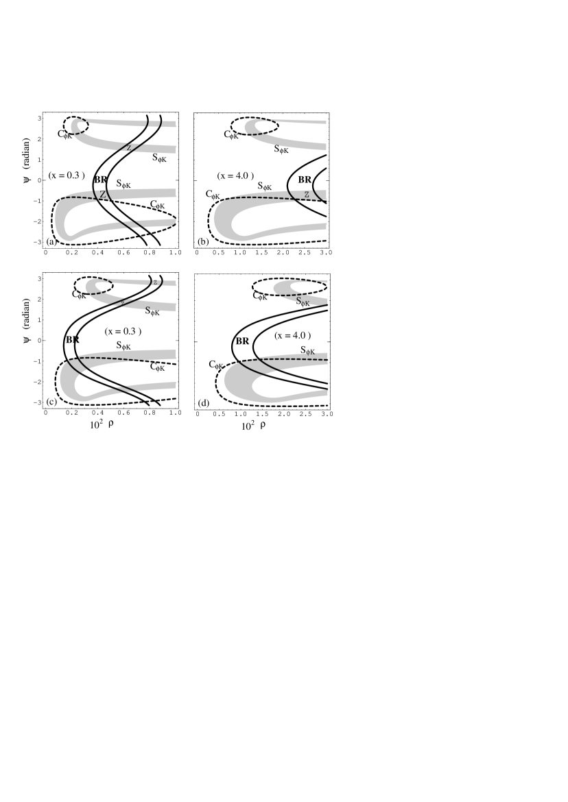
Figure 2: Contour plots of $S_{\phi K},C_{\phi K}$ and ${\cal B}(B\to\phi K_{S})$ in $\rho-\psi$ plane for two values of $x=0.3~{}(a,c)$ and $4.0~{}(b,d)$ for $LR(RL)$ mixing with $m_{\tilde{q}}=500$ GeV. The scale $\mu=m_{b}$ for Figures $(a)$ and $(b)$, while it is $m_{b}/2$ for Figures $(c)$ and $(d)$. The $1\sigma$ allowed regions of $S_{\phi K}$, ${\cal B}$ and $C_{\phi K}$ are two gray bands, area within the solid curves and area outside the two dotted contours respectively.

In our analysis we consider $m_{\tilde{q}}=500$ GeV and take two values of $x=0.3$ and $4.0$, which will determine the gluino masses. In Figure 2 we show the $1\sigma$ allowed region in $\rho-\psi$ plane from $B\to\phi K$ data on $S_{\phi K},C_{\phi K}$ and ${\cal B}$. The gray band indicate the parameter space which is allowed by $S_{\phi K}$. The area outside the two dotted contours is allowed by $C_{\phi K}$, while the area enclosed by the solid curves is allowed by the ${\cal B}(B\to\phi K_{S})$ measurement. The region (marked by $Z$) in gray band enclosed by the solid curves is the only parameter space left in $\rho-\psi$ plane which is allowed by the experimentally measured $S_{\phi K},C_{\phi K}$ and ${\cal B}$ within $1\sigma$.

The Figures 2$(a)$ and $(b)$ , correspond to contour plots for $x=0.3$ and $4.0$ respectively at the scale $\mu=m_{b}$. For $x=0.3$, we get two allowed regions each at positive and negative values of the new phase $\psi$. On the other hand for $x=4.0$, we get only one allowed region which lies at the negative value of $\psi$ and at much higher value of $\rho>2.2\times 10^{-2}$. We have noticed before that the constraint on $LR(RL)$ mixing parameter from the ${\cal B}(B\to X_{s}\gamma)$ is stronger at $x=0.3$ compared to the limit at $x=4.0$. This behavior is also reflected in the $B\to\phi K$ process, where we find that, for $x=4.0$, the $1\sigma$ constraint from $S_{\phi K},C_{\phi K}$ and ${\cal B}$ is much weaker compared to the constraint shown in Figure 2$(a)$ correspond to $x=0.3$.

Similar allowed regions are shown in Figure 2$(c)$ for a different choice of the QCD scale $\mu=m_{b}/2$. One can see that the allowed parameter space does depend on $\mu$. In this case, both the allowed regions are confined at the positive value of $\psi$. For $x=4.0$ ( Figure 2$(d)$), there are no allowed regions. From the $S_{\phi K}$ and branching ratio contour one can see that the allowed region from $B\to\phi K$ require some higher value of $\rho$ which lies beyond $B\to X_{s}\gamma$ limit.

Before we conclude this section, we would like to compare our predictions with some of the existing literatures on $B\to\phi K$ process [10, 11, 17].

We agree qualitatively with the results of Ref.[11, 17] in places where we overlap. Similar to our approach, both of these analyses were based upon the QCD improved factorization scheme. However, there are some quantitative differences between these papers and our analysis. For example, we differ in the choice of squark and gluino masses, the authors of the above two papers considered degenerate squark and gluino masses, whereas we have considered non-degenerate squark-gluino masses. We have fixed the squark mass at 500 GeV and considered two values of the gluino masses, determined by the parameter $x$ defined earlier. Secondly, we have performed our analysis for two values the QCD scale, $\mu=m_{b}/2$ and $m_{b}$. Our results depend strongly on the choice of the ratio $x$ and also on the scale $\mu$. However, in a broad sense, we do agree that to satisfy $B\to\phi K$ data, one requires $\mid\delta^{bs}_{LR(RL)}\mid\sim 10^{-3}-10^{-2}$.

In Ref.[10], authors made a detailed investigation of a scenario in which the $LR$ and $RR$ operators co-exist. Moreover, because of the large mixing, the calculation was done in the mass eigenbasis with more model dependence than ours. It has been shown in this analysis that $RR$ insertion (which arises due to a large mixing between $\tilde{s}_{R}$ and $\tilde{b}_{R}$) could show sizable effect on $S_{\phi K}$, but only for very light gluino mass, near the experimental bound. Such a large $RR$ mixing also modify $\Delta M_{s}$ significantly which can be observed at the Tevatron Run II. In their second case, they have the combination of both large right-right and left-right squark mixing ($LR+RR)$. In this case the squark and gluinos could be sufficiently heavy to have no significant enhancement of the $\Delta M_{s}$.

From our analysis we observe that SUSY leads to a comprehensive understanding of $B\to\phi K_{S}$ data though in a very limited parameter space of $\delta^{bs}_{LR(RL)}$. In rest of the paper we now explore the consequence of such $LR(RL)$ mixing of squarks in the $B\to\phi K^{\ast}$ process.

6 $B\to\phi K^{\ast}$ decay

In this section we will study the effect of $LR(RL)$ mixing of down type squarks to $B\to\phi K^{\ast}$ process through the gluonic dipole moment operator $C_{8g}$. We will study the $B\to\phi K^{\ast}$ process by using the QCD improved factorization. Using this method one can compute nonfactorizable corrections to the above process in the heavy quark limit. Recently the $B\to VV$ process has been computed using QCD improved factorization method [37]. In rest of analysis we will follow Ref. [37].

The most general Lorentz invariant decay amplitude for the process $B\to VV$ can be expressed as

$${\cal M}(B(p_{B})\to V_{1}(\epsilon_{1},p_{1})V_{2}(\epsilon_{2},p_{2}))\propto\epsilon^{\ast\mu}_{1}\epsilon^{\ast\nu}_{2}\left[ag_{\mu\nu}+bp_{B\mu}p_{B\nu}+ic\epsilon_{\mu\nu\alpha\beta}p^{\alpha}_{1}p^{\beta}_{2}\right]$$ (24)

where the coefficients $c$ correspond to the $p$-wave amplitude, and $a,b$ to the mixture of $s$ and $d$ wave amplitudes. Using these $a,b$ and $c$ coefficients one can construct the three helicity amplitudes:

$$H_{00} = \frac{1}{2m_{V_{1}}m_{V_{2}}}\left[(m^{2}_{B}-m^{2}_{V_{1}}-m^{2}_{V_{2}})a+2m^{2}_{B}p^{2}_{cm}b\right]\$$

$$H_{\pm\pm} = a\mp m_{B}p_{cm}c$$ (25)

where $p_{cm}$ is the center of mass momentum of the vector meson in the $B$ rest frame and $m_{V_{1}}(m_{V_{2}})$ is the mass of the vector meson $V_{1}(V_{2})$. These helicity amplitudes $H_{00}$ and $H_{\pm\pm}$ can be related to the spin amplitudes in the transverse basis $(A_{0},A_{\mid\mid},A_{\perp})$ defined in terms of linear polarization of the vector mesons:

$$A_{0} = H_{00}$$

$$A_{\mid\mid} = \frac{1}{\sqrt{2}}\left(H_{++}+H_{--}\right)$$

$$A_{\perp} = \frac{1}{\sqrt{2}}\left(H_{++}-H_{--}\right)$$ (26)

Branching ratio	Data	Weighted average
$B^{+}\to\phi K^{*+}$	BaBar     $\left(12.1^{+2.1}_{-1.9}\pm 1.5\right)\times 10^{-6}$
	CLEO      $\left(10.6_{-4.9-1.6}^{+6.4+1.8}\right)\times 10^{-6}$	$\left(9.9\pm 1.23\right)\times 10^{-6}$
	Belle     $\left(9.4\pm 1.1\pm 0.7\right)\times 10^{-6}$
$\bar{B}^{0}\to\phi\bar{K}^{*0}$	BaBar     $\left(11.1_{-1.2}^{+1.3}\pm 1.1\right)\times 10^{-6}$
	CLEO     $\left(11.5_{-3.7-1.7}^{+4.5+1.8}\right)\times 10^{-6}$	$\left(10.6\pm 1.3\right)\times 10^{-6}$
	Belle     $\left(10_{-1.5-0.8}^{+1.6+0.7}\right)\times 10^{-6}$

Table 1: Experimental data of $B\to\phi K^{\ast}$ decays from BaBar [40], CLEO [41] and Belle [42] and their weighted average.

The decay rate can be written as

$$\Gamma(B\to V_{1}V_{2})=\frac{p_{cm}}{8\pi m^{2}_{B}}\left[\mid H_{00}\mid^{2}+\mid H_{++}\mid^{2}+\mid H_{--}\mid^{2}\right]$$ (27)

Neglecting the annihilation contributions (which are expected to be small) to $B\to\phi K^{\ast}$, $H_{00}$ and $H_{\pm\pm}$ are given by:

$$H_{00} = \frac{G_{F}}{\sqrt{2}}\frac{a^{n}(\phi K^{\ast})f_{\phi}}{2m_{K^{\ast}}}\Bigg{\{}\left(m^{2}_{B}-m^{2}_{K^{\ast}}-m^{2}_{\phi}\right)\left(m_{B}+m_{K^{\ast}}\right)A^{BK^{\ast}}_{1}(m^{2}_{\phi})$$

$$-\frac{4m^{2}_{B}p^{2}_{c}}{m_{B}+m_{K^{\ast}}}A^{BK^{\ast}}_{2}(m^{2}_{\phi})\Bigg{\}}$$

$$H_{\pm\pm} = \frac{G_{F}}{\sqrt{2}}a^{n}(\phi K^{\ast})m_{\phi}f_{\phi}\Bigg{\{}\left(m_{B}+m_{K^{\ast}}\right)A^{BK^{\ast}}_{1}(m^{2}_{\phi})$$ (28)

$$\mp\frac{2m_{B}p_{c}}{m_{B}+m_{K^{\ast}}}V^{BK^{\ast}}(m^{2}_{\phi})\Bigg{\}}$$

where, $a^{n}(\phi K^{\ast})=a^{n}_{3}+a^{n}_{4}+a^{n}_{5}-(a^{n}_{7}+a^{n}_{9}+a^{n}_{10})/2$. The effective parameters $a_{i}$ appearing in the helicity amplitudes $H_{00}$ and $H_{\pm\pm}$ given in Ref.[37, 24] and other input parameters are given in Ref.[24].

In Table 1, we display the experimentally (BaBar, CLEO and Belle) measured branching ratios and the weighted averaged values for the $B^{+}\to\phi K^{\ast+}$ and $\bar{B}^{0}\to\phi\bar{K}^{\ast 0}$. The theoretical predictions in the SM for two different form factor models, the LCSR and BSW models are given in Ref.[37].

$x$	$(\rho,\psi)$	${\cal B}^{\rm SUSY}$ (in units of $10^{-6}$)	${\cal A}_{CP}$ (in $\%$)
	($0.4\times 10^{-2}$, -0.5)	$23.37^{+4.88}_{-4.42}~{}~{}(21.76^{+4.56}_{-4.13})$	$-4.7(-4.4)$
0.3	($0.4\times 10^{-2}$, -0.7)	$21.50^{+4.49}_{-4.06}~{}~{}(20.17^{+4.22}_{-3.83})$	$-7.0~{}~{}(-6.5)$
	($0.6\times 10^{-2}$, 1.5)	$27.46^{+5.75}_{-5.2}~{}~{}(26.82^{+5.62}_{-5.08})$	$17.7~{}~{}(15.7)$
	$(2.4\times 10^{-2},-0.5)$	$24.33^{+5.08}_{-4.6}~{}~{}(22.65^{+4.75}_{-4.3})$	$-4.7~{}~{}(-4.4)$
4.0	($2.6\times 10^{-2}$, -0.45)	$26.98^{+5.6}_{-5.1}~{}~{}(25.11^{+5.27}_{-4.76})$	$-4.2~{}~{}(-3.9)$
	($2.8\times 10^{-2}$, -0.8)	$25.31^{+5.3}_{-4.8}~{}~{}(23.87^{+5.01}_{-4.52})$	$-8.0~{}~{}(-7.5)$

Table 2: ${\cal B}(B^{+}\to\phi K^{\ast+})$ and ${\cal A}_{CP}(B^{+}\to\phi K^{\ast+})$ at the QCD scale $\mu=m_{b}$ for $LR$ mass insertion for selected points in the allowed $\rho-\psi$ space. The numbers in the parenthesis correspond to the $RL$ mass insertion. The standard model branching ratio corresponding to this scale is $(6.18^{+1.29}_{-1.15})\times 10^{-6}$. The errors are due to $\pm 10\%$ theoretical uncertainties in the calculation.

6.1 $LR(RL)$ mixing contributions to $B\to\phi K^{\ast}$

In this section we will study the effect of $LR(RL)$ mixing in $B\to\phi K^{\ast}$ process. This $LR(RL)$ mass insertion can enhance the Wilson coefficient $C_{8g}$ by a factor of $m_{\tilde{g}}/m_{b}$ compared to the standard model contribution in the same way as shown in section 5 for $B\to\phi K$ process. Hence, one need to impose the constrain on $LR(RL)$ mixing from experimentally measured ${\cal B}(B\to X_{s}\gamma)$ and also from $S_{\phi K},C_{\phi K}$ and ${\cal B}(B\to\phi K)$ as obtained section 5.

In this scenario, the new weak phase $\psi$, (the phase of the $LR(RL)$ mixing ) will contribute to direct CP-violating asymmetry ${\cal A}_{CP}$ defined as :

$${\cal A}_{CP}=\frac{\Gamma(B^{+}\to\phi K^{\ast+})-\Gamma(B^{-}\to\phi K^{\ast-})}{\Gamma(B^{+}\to\phi K^{\ast+})+\Gamma(B^{-}\to\phi K^{\ast-})}$$ (29)

in terms of partial widths. Recently BaBar and Belle Collaboration has presented their measurement of CP violating asymmetries for $B^{0}\to\phi K^{\ast 0}$ and $B^{\pm}\to\phi K^{\ast\pm}$ [40, 42]

$${\cal A}_{CP}(\bar{B}^{0}\to\phi\bar{K}^{\ast 0}) = 0.04\pm 0.12\pm 0.02,~{}~{}~{}0.07\pm 0.15^{+0.05}_{-0.03}$$ (30)

$${\cal A}_{CP}(B^{\pm}\to\phi K^{\ast\pm}) = +0.16\pm 0.17\pm 0.04,~{}~{}~{}-0.13\pm 0.29^{+0.08}_{-0.11}$$ (31)

where, in each asymmetry result, the first number correspond to the BaBar data while the second one correspond to Belle measurement. The standard model value for this asymmetry is less than $1\%$. The new physics (SUSY) contributions from the new penguin operator appeared due to $LR(RL)$ mixing $(\delta^{bs}_{LR(RL)})$ can modify the sign and magnitude of ${\cal A}_{CP}(B^{\pm}\to\phi K^{\ast\pm})$ within the allowed parameter space of $\delta^{bs}_{LR(RL)}$.

$x$	$(\rho,\psi)$	${\cal B}^{\rm SUSY}$ (in units of $10^{-6}$)	${\cal A}_{CP}$ (in $\%$)
	($0.55\times 10^{-2}$, 1.8)	$31.83^{+6.6}_{-6.0}~{}~{}(32.45^{+6.7}_{-6.1})$	$19.39^{+0.01}_{-0.02}~{}~{}(16.17^{+0.05}_{-0.07})$
0.3	($0.82\times 10^{-2}$, 2.8)	$14.50^{+3.04}_{-2.74}~{}~{}(21.62^{+4.44}_{-4.02})$	$20.2~{}~{}(10.96^{+0.06}_{-0.08})$
	($0.82\times 10^{-2}$, 2.9)	$12.39^{+2.59}_{-2.34}~{}~{}(19.82^{+4.05}_{-3.67})$	$15.73~{}~{}(8.04^{+0.05}_{-0.06})$

Table 3: ${\cal B}(B^{+}\to\phi K^{\ast+})$ and ${\cal A}_{CP}(B^{+}\to\phi K^{\ast+})$ at the QCD scale $\mu=m_{b}/2$ for $LR$ mass insertion for selected points in the allowed $\rho-\psi$ space. The numbers in the parenthesis correspond to the $RL$ mass insertion. The standard model branching ratio corresponding to this scale is $(14.92^{+3.08}_{-2.78})\times 10^{-6}$. The errors are due to $\pm 10\%$ theoretical uncertainties in the calculation.

To get the numerical values of ${\cal B}(B^{+}\to\phi K^{\ast+})$, and ${\cal A}_{CP}(B^{+}\to\phi K^{\ast+})$, we fix $x=0.3$ and $4.0$. Then for a given QCD scale $\mu$, we select some points in the allowed parameter space of $\rho-\psi$ plane (as marked by $Z$ in Figure 2) for both values of $x$. In this computation, we include $(\pm 10\%)$ theoretical uncertainties.

In Table 2, we present the branching ratio ${\cal B}(B^{+}\to\phi K^{\ast+})$ and the CP rate asymmetry ${\cal A}(B^{+}\to\phi K^{\ast+})$ for $\mu=m_{b}$ and selected values of $x=0.3$ and $4.0$ for values of $\rho$ and $\psi$ allowed by $B\to\phi K_{S}$ data for $LR$ mass insertion ($RL$ is shown in the parenthesis). The branching ratio with SUSY turn out to be much higher than the standard model value of $6.18^{+1.29}_{-1.15}$, which is lower than the experimental data (Table 1). Even the lower range of theory prediction is much higher than the upper range of experimental data within $1\sigma$. The rate asymmetry has much less error and is consistently within the range $\sim-4\%$ to $\sim 18\%$.

Similarly in Table 3, we show ${\cal B}$ and ${\cal A}_{CP}$ calculated for QCD scale $\mu=m_{b}/2$. In this case, there are two allowed regions from the combined $B\to\phi K$ and $B\to X_{s}\gamma$ constraints corresponding to $x=0.3$. For $x=4.0$, there are no allowed regions from $B\to\phi K$ data. The standard model branching ratio is much larger compared to the one computed at $\mu=m_{b}$. In SUSY, apart from the QCD scale $\mu$, the branching ratio also depend on the values of $\rho$ and $\psi$. Moreover, the selected points in $\rho-\psi$ plane are different in the two cases. In the case, with $\mu=m_{b}/2$, and at $\rho=0.82\times 10^{-2}$ and $\psi=2.8,2.9$ radians, with $LR$ mixing, lower ranges of the theory predictions are consistent with the upper range of experimental data at one sigma. For the other value of $\rho$ and $\psi$, the theoretical prediction for branching ratio is much higher than the standard model theory as well as experimental data. With $RL$ mixing, the predicted branching ratio is much larger compared to both the standard model prediction and experimental data. The asymmetries for both $LR$ and $RL$ mixing case are always positive with less errors.

We conclude that for some selected points in $\rho-\psi$ plane allowed by $B\to\phi K$ and $B\to X_{s}\gamma$ at $\mu=m_{b}/2$ provide a satisfactory understanding of $B\to\phi K^{\ast}$ process. We also note that, at $\mu=m_{b}$ the SUSY contribution to the branching ratio of $B\to\phi K^{*}$ is too large to be consistent with the experimental data.

We have also studied other CP violating asymmetries that can arise in vector-vector final state. The set of observables are defined in terms of $A_{0},A_{\mid\mid}$ and $A_{\perp}$ as follows [26].

$$\Lambda_{\lambda}\,=\,\frac{|A_{\lambda}|^{2}+|\bar{A}_{\lambda}|^{2}}{2},~{}~{}~{}~{}\Sigma_{\lambda\lambda}=\frac{\mid A_{\lambda}\mid^{2}-\mid\bar{A}_{\lambda}\mid^{2}}{2},$$

$$\Lambda_{\perp i}\,=\,-\,{\rm Im}\left(A_{\perp}A_{i}^{*}-\bar{A}_{\perp}\bar{A}_{i}^{*}\right),~{}~{}~{}~{}\Lambda_{\mid\mid 0}={\rm Re}\left(A_{\mid\mid}A^{\ast}_{0}+\bar{A}_{\mid\mid}\bar{A^{\ast}}_{0}\right),$$

$$\Sigma_{\perp i}=-{\rm Im}\left(A_{\perp}A^{\ast}_{i}+\bar{A}_{\perp}\bar{A^{\ast}}_{i}\right),~{}~{}~{}~{}\Sigma_{\mid\mid 0}={\rm Re}\left(A_{\mid\mid}A^{\ast}_{0}-\bar{A}_{\mid\mid}\bar{A^{\ast}}_{0}\right),$$

$$\rho_{\perp i}={\rm Re}\left(\frac{q}{p}\left[A^{\ast}_{\perp}\bar{A}_{i}+A^{\ast}_{i}\bar{A}_{\perp}\right]\right),~{}~{}~{}~{}\rho_{\perp\perp}={\rm Im}\left(\frac{q}{p}A^{\ast}_{\perp}\bar{A}_{\perp}\right),$$

$$\rho_{\mid\mid 0}=-{\rm Im}\left(\frac{q}{p}\left[A^{\ast}_{\mid\mid}\bar{A}_{0}+A^{\ast}_{0}\bar{A}_{\mid\mid}\right]\right),~{}~{}~{}~{}\rho_{ii}=-{\rm Im}\left(\frac{q}{p}A^{\ast}\bar{A}_{i}\right)$$ (32)

where $\lambda=\{0,\,\parallel,\,\perp\}$ and the observables where $i=\{0,\,\parallel\}$, We restrict ourselves to the study of helicity dependent $CP$ asymmetry defined as $\Sigma_{\lambda\lambda}/\Lambda_{\lambda\lambda}$  [26]. For the purpose of illustration we select last two sample points from the Table 3. At these values of $\rho$ and $\psi$, with $LR$ mass insertion, the lower range of the ${\cal B}^{SUSY}$ is consistent with the upper range of the experimental data on ${\cal B}(B\to\phi K^{*})$ at one sigma. We then compute $\Sigma_{\lambda\lambda}/\Lambda_{\lambda\lambda}$ for each values of $\lambda$ for these two sets of $\rho$ and $\psi$ and is shown in Table 4. As before, in this case also we include $\pm 10\%$ theoretical uncertainties in our calculation. We only show the helicity dependent asymmetries for $LR$ mass insertion, since with $RL$ mass insertion the SUSY contribution to the branching ratio is too large to be consistent with the data.

$x$	$(\rho,\psi)$	$\Sigma_{00}/\Lambda_{00}$	$\Sigma_{\mid\mid}/\Lambda_{\mid\mid}$	$\Sigma_{\perp\perp}/\Lambda_{\perp\perp}$
0.3	($0.82\times 10^{-2}$, 2.8)	$0.19\pm 0.00$	$0.61^{+0.009}_{-0.012}$	$0.57^{+.011}_{-0.013}$
	($0.82\times 10^{-2}$, 2.9)	$0.15\pm 0.00$	$0.71^{+0.020}_{-0.026}$	$0.65^{+0.022}_{-0.027}$

Table 4: Helicity dependent CP asymmetry at the QCD scale $\mu=m_{b}/2$ for $LR$ mass insertion for selected points in the allowed $\rho-\psi$ space. The errors consist of $\pm 10\%$ theoretical uncertainties.

7 Conclusions

In this talk, we considered the SUSY contribution to the gluonic dipole moment operator to $B\to\phi K_{S}$ process. We found that the $LR(RL)$ mass insertion can enhance the gluonic dipole moment operator significantly. We then used the experimentally measured quantities, such as $S_{\phi K},C_{\phi K}$ and ${\cal B}(B\to\phi K_{S})$ to constrain the parameter space of $LR(RL)$ mixing. Interestingly, we find that the constraints from $B\to\phi K$ data is consistent with the $B\to X_{s}\gamma$ limit. It turned out that the same enhancement of gluonic dipole moment operator could also affect other penguin dominated process, such as $B\to\phi K^{\ast}$, which is a pure penguin process like $B\to\phi K_{S}$. In standard model, the predicted ${\cal A}_{CP}(B\to\phi K^{\ast})$ is less than $1\%$. We calculated such asymmetries and also the branching ratio for the set of parameters allowed by $B\to\phi K$ data. At $\mu=m_{b}$, for both $LR$ and $RL$ mass insertion, we observed that the predicted branching ratio is well above the experimentally measured one. On the other hand, at the QCD scale $\mu=m_{b}/2$ with $LR$ mass insertion, we found that the theoretically computed branching ratio is consistent with the data with in one sigma error. At this second choice of allowed parameter space of $\delta^{bs}_{LR(RL)}$, we found ${\cal A}_{CP}(B^{+}\to\phi K^{\ast+})$ in the range $15\%$ to $20\%$, which is significantly higher than the standard model prediction but is still consistent with the present data. Finally, we also presented helicity dependent CP asymmetries in the same parameter space of $\delta^{bs}_{LR}$.

Acknowledgments

This work was supported in part by US DOE contract numbers DE-FG03-96ER40969.

References

- [1] B. Aubert et al.[BaBar Collaboration], arXiv:hep-ex/0207070.
- [2] K. Abe et al.[Belle Collaboration], arXiv:hep-ex/0207098
- [3] K. Abe et al.[Belle Collaboration], Phys. Rev. D 67, 031102 (2003) .
- [4] G. Hamel De Monchenault, arXiv:hep-ex/0305055.
- [5] R. Barbieri and A. Strumia, Nucl. Phys. B508, 3 (1997) .
- [6] A. Kagan, arXiv:hep-ph/9806266; talk at the 2nd International Workshop on B physics and CP Violation, Taipei, 2002; SLAC Summer Institute on Particle Physics, August 2002.
- [7] G. Hiller, Phys. Rev. D 66, 071502 (2002) .
- [8] A. Datta, Phys. Rev. D 66, 071702 (2002) .
- [9] M.Ciuchini and L. Silvestrini, Phys. Rev. Lett. 89, 231802 (2002);
- [10] R. Harnik, D. T. Larson, H. Murayama and A. Pierce, Phys. Rev. D 69, 094024 (2004) .
- [11] M. Ciuchini, E. Franco, A. Masiero and L. Silvestrini, Phys. Rev. D 67, 075016 (2003) [Erratum-idib. D 68, 079901 (2003)].
- [12] B. Dutta, C.S. Kim and S. Oh, Phys. Rev. Lett. 90, 011801 (2003).
- [13] S. Khalil and E. Kou, Phys. Rev. D 67, 055009 (2003) .
- [14] C.W. Chiang and J.L. Rosner, Phys. Rev. D 68, 014007 (2003) .
- [15] A. Kundu and T. Mitra, Phys. Rev. D 67, 116005 (2003) .
- [16] K. Agashe and C.D. Carone, Phys. Rev. D 68, 035017 (2003) .
- [17] G.L. Kane, P. Ko, H. b. Wang, C. Kolda, J.h. Park and L.T. Wang, Phys. Rev. Lett. 90, 141803 (2003).
- [18] D. Chakraverty, E. Gabrielli, K. Huitu and S. Khalil, Phys. Rev. D 68, 095004 (2003) .
- [19] J.F. Cheng, C.S.Huang and X.h. Wu, Phys. Lett. B585, 287 (2004).
- [20] R. Arnowitt, B. Dutta and B. Hu, Phys. Rev. D 68, 075008 (2003) .
- [21] E. Gabrielli, K. Huitu and S. Khalil, arXiv: hep-ph/0407291.
- [22] K. Abe et al.[Belle Collaboration], Phys. Rev. Lett. 91, 261602 (2003). T. Browder, CKM Phases (), Talk presented at Lepton-Photon 2003.
- [23] A.J. Buras, arXiv:hep-ph/0210291.
- [24] C. Dariescu, M.A. Dariescu, N.G. Deshpande and D. K. Ghosh, Phys. Rev. D 69, 112003 (2004) .
- [25] M. Beneke, G. Buchalla, M. Neubert and C.T. Sachrajda, Phys. Rev. Lett. 83, 1914 (1999) ; Nucl. Phys. B591, 313 (2000); Nucl. Phys. B606, 245 (2001).
- [26] D. London, N. Sinha, and R. Sinha, Phys. Rev. Lett. 85, 1807 (2000).
- [27] R.A. Briere et al., [CLEO Collaboration], Phys. Rev. Lett. 86, 3718 (2002).
- [28] X.-G. He, J.P. Ma and C.-Y. Wu, Phys. Rev. D 63, 094004 (2001) ;
- [29] C.-S. Huang and S. Zhu, Phys. Rev. D 68, 114020 (2003) .
- [30] L.J. Hall, V.A.Kostelecky and S. Raby, Nucl. Phys. B267, 415 (1986) .
- [31] F. Gabbiani, E. Gabrielli, A. Masiero and L. Silvestrini, Nucl. Phys. B477, 321 (1996) .
- [32] M. B. Causse and J. Orloff, Eur. Phys. J. C23,749 (2002) ; S. Khalil and E. Kou in Ref.[5].
- [33] A.J. Buras, G. Colangelo, G. Isidori, A. Romanino, and L. Silvestrini, Nucl. Phys. B566, 3 (2000).
- [34] X.-G. He, J.-Y. Leou and J.-Q. Shi, Phys. Rev. D 64, 094018 (2001) .
- [35] A. Ali, G. Kramer and Cai-Dian Lu, Phys. Rev. D 58, 094009 (1998) .
- [36] A. Stocchi, Phys. Proc. Suppl. 117, 145 (2003).
- [37] H.-Y. Cheng and K.-C. Yang, Phys. Lett. B511, 40 (2001).
- [38] P. Ball and V.M. Braun, Phys. Rev. D 58, 094016 (1998) ; P. Ball, J. High Energy Phys.09, 005 (1998).
- [39] M. Wirbel, B. Stech and M. Bauer, Z. Phys. C29, 637 (1985) ; M. Bauer, B. Stech and M. Wirbel, Z. Phys. C34, 103 (1987) .
- [40] B. Aubert et al., [BaBar Collaboration], Phys. Rev. Lett. 91, 171802 (2003); ibid 93,231804 (2004).
- [41] R.A. Briere et al., [CLEO Collaboration], Phys. Rev. Lett. 86, 3718 (2001).
- [42] K.-F. Chen et al., [Belle Collaboration], Phys. Rev. Lett. 91, 201801 (2003).