Bohr-Sommerfeld quantization and meson spectroscopy

Abstract

We use the Bohr-Sommerfeld quantization approach in the context of constituent quark models. This method provides, for the Cornell potential, analytical formulae for the energy spectra which closely approximate numerical exact calculations performed with the Schrödinger or the spinless Salpeter equations. The Bohr-Sommerfeld quantization procedure can also be used to calculate other observables such as r.m.s. radius or wave function at the origin. Asymptotic dependence of these observables on quantum numbers are also obtained in the case of potentials which behave asymptotically as a power-law. We discuss the constraints imposed by these formulae on the dynamics of the quark-antiquark interaction.

I Introduction

It is well known that nonrelativistic or semirelativistic constituent quark models can describe with surprising accuracy a large part of the meson and baryon properties. The mass spectra of hadrons have been intensively studied since the pioneering works of, e.g., Eichten et al. eich75 , Stanley and Robson stan80 and Godfrey and Isgur godf85 (see for example luch91 ; fulc94 ; brau98 ). Other observables, such as decay widths, have also been well reproduced within the framework of potential models godf85 . The success of these calculations shows that it is possible to understand the major part of the hadron observables using the simple picture for the quark-quark or quark-antiquark interaction provided by constituent quark models.

In this paper, we will focus on the meson spectroscopy. Many potentials have been proposed to describe the meson properties luch91 ; brau98 . Despite of this diversity, the central part of the interaction used in usual models presents similar characteristics: an attractive short range part with a confining long range interaction. The prototype for these potentials is the so-called Cornell potential eich75 which can be used to describe a large body of the meson masses except the masses of the pseudoscalar states for which a spin dependent and a flavor mixing interaction is necessary. Indeed, the role of this additional interaction is too important, in this sector, to be neglected even in a first approximation. Recent lattice calculations bali97 confirm that the Cornell potential fits in a good approximation the static quark-antiquark interaction.

Most of the models found in Refs. luch91 ; brau98 have a phenomenological nature: whereas the general behavior of potentials are often dictated by physical considerations, the values of their parameters are most of the time obtained by trial and error from a comparison with some experimental data. The values of various observables which can be generated from potential models will be strongly constrained by this general behavior of potentials and by the values of their parameters; however, despite of the ease with which the numerical values of these observables can be obtained, the exact nature of these constraints is often very difficult to infer from the numerical results.

It is the purpose of this work to show that the use of a Bohr-Sommerfeld quantization (BSQ) approach can provide unexpected insight into potential models. We use this method to obtain some general characteristics of constituent quark models. In particular, we will show that it is possible to obtain analytical expressions for the spectra, root mean square radii, decay widths, electromagnetic mass splittings or electric polarizabilities, which closely approximate the numerically exact results obtained from full quantum Schrödinger or spinless Salpeter approaches, and which can thus be used, e.g., to derive accurate predictions for the dependence of the observables on the quantum numbers. We will study the constraints imposed by these formulae on the dynamics of the quark-antiquark interaction within a potential model.

II The BSQ Method

The basic quantities in the BSQ approach tomo62 are the action variables,

$$J_{s}=\oint p_{s}\,dq_{s},$$ (1)

where $s$ labels the degrees of freedom of the system, and where $q_{s}$ and $p_{s}$ are the coordinates and conjugate momenta; the integral is performed over one cycle of the motion. The action variables are quantized according to the prescription

$$J_{s}=(n_{s}+c_{s})\,h,$$ (2)

where $h$ is Planck’s constant, $n_{s}$ ($\geq 0$) is an integral quantum number and $c_{s}$ is some real constant, which according to Langer should be taken equal to $1/2$ lang37 .

To draw some general conclusions about potential models applied to meson spectroscopy we use the BSQ formalism, in the next sections, with the Cornell potential. The properties of various observables are representative of those which can be obtained from the usual constituent quark models. In particular, conclusions about asymptotic behaviors (large value of quantum numbers) of these quantities will be quite reliable since most of the potential models use a linear confinement. Moreover, we will show that we can also obtain information about asymptotic behaviors for any power-law confinement.

II.1 Nonrelativistic calculations

The nonrelativistic Hamiltonian corresponding to the Cornell potential reads in natural units $(\hbar=c=1)$:

$$H=\frac{1}{2\mu}\left(p_{r}^{2}+\frac{p_{\phi}^{2}}{r^{2}}\right)-\frac{\kappa}{r}+a\,r.$$ (3)

Of course since the interaction is central, the orbital angular momentum $p_{\phi}=L$ is a constant of the motion. The expression for the radial momentum $p_{r}$ derives from the conservation of the total energy $E$ of the system,

$$p_{r}=\pm\,\frac{1}{r}\,\sqrt{-2\mu a\,r^{3}+2\mu E\,r^{2}+2\mu\kappa\,r-L^{2}}=\pm\,\frac{1}{r}\,\sqrt{g(r)}.$$ (4)

The radial motion takes place between two turning points, $r_{-}$ and $r_{+}$, which are the two positive zeros of $g(r)$; the three roots, $r_{k}$ ($k=0,1,2$), of $g(r)$ are

$$r_{k}=2\,\sqrt{\frac{-P}{3}}\,\cos\left(\frac{\theta+2\pi k}{3}\right)+\frac{E}{3a},$$ (5)

where

$$P = -\frac{1}{3a^{2}}\left(E^{2}+3a\kappa\right),\quad\cos\theta=-\frac{Q}{2}\sqrt{\frac{27}{-P^{3}}},$$

$$Q = -\frac{1}{27a^{3}}\left(2E^{3}+9a\kappa E-27\frac{a^{2}}{2\mu}L^{2}\right).$$ (6)

As $r_{1}\leq 0\leq r_{2}\leq r_{0}$, the turning points are $r_{-}=r_{2}$ and $r_{+}=r_{0}$.

Quantization of $J_{\phi}$ trivially gives $L=\ell+c_{\phi}$; on the other hand, quantization of $J_{r}$ leads to the equation

$$2\mu\,r_{+}\,(Er_{1}+2\kappa)\,K(\eta)+2\mu\,E\,r_{+}\,(r_{+}-r_{1})\,E(\eta)-3(\ell+c_{\phi})^{2}\,\Pi(\pi/2,\gamma,\eta)-$$

$$\frac{3}{2}\pi\,(n+c_{r})r_{+}\sqrt{r_{+}-r_{1}}\,\sqrt{2\mu\,a}=0,$$ (7)

where

$$\eta=\frac{r_{+}-r_{-}}{r_{+}-r_{1}}\quad\text{and}\quad\gamma=1-\frac{r_{-}}{r_{+}},$$ (8)

$K(x)$, $E(x)$ and $\Pi(\pi/2,x,y)$ are the complete elliptic integrals of the first, second and third kind, respectively (grad80, , p. 904), and $n$ is the radial quantum number. This appears to be a rather complicated equation since it cannot be solved explicitly for the energy. However, it leads to very accurate results if we choose the Langer prescription $c_{r}=c_{\phi}=1/2$, as it can be seen in Table 1 where a selected set of masses, computed from Eq. (II.1), are compared with the results of an exact calculation fulc94 . The accuracy of the results presented in Table 1 is representative of that obtained for the states which are not displayed here. One sees that, even for small quantum numbers, the errors introduced by the BSQ approximation are remarkably small; indeed the errors in the spectrum reported in Table 1 do not exceed $0.1\%$.

One of the most useful byproducts of the BSQ method is to provide simple asymptotic expressions for the total energy for large values of $\ell$ and $n$. Indeed, for large angular momenta ($\ell\gg n$), the orbits become almost circular, and thus $r_{-}\approx r_{+}$ and $\eta\approx 0$. In this limit, $\theta=\pi$ and all the elliptic integrals are equal to $\pi/2$; keeping the leading terms in Eq. (II.1), we obtain:

$$E\sim\frac{3}{2}\left(\frac{a^{2}}{\mu}\right)^{1/3}\ell^{2/3}\quad\quad(\ell\gg n).$$ (9)

This is a well-known result: a linear potential does not lead to linear Regge trajectories in a nonrelativistic description; correct Regge trajectories can only be obtained with confining potentials rising as $r^{2/3}$ fabr88 .

For large radial quantum numbers ($n\gg\ell$), the orbits have a large eccentricity, and thus $r_{1}\approx r_{-}\approx 0$ and $\eta\approx 1$. Although $\eta=1$ cannot be directly inserted into Eq. (II.1) because of the singularity of the elliptic integrals, setting $r_{1}=r_{-}=0$ into Eq. (1) and evaluating an elementary integral leads to:

$$E\sim\left(\frac{3\pi}{2}\right)^{2/3}\left(\frac{a^{2}}{2\mu}\right)^{1/3}n^{2/3}\quad\quad(n\gg\ell).$$ (10)

This is a new result: the radial quantum number does not appear explicitly in the classical Hamiltonian, and thus “naive” semiclassical methods fail to reproduce correctly the spectrum in this sector shee81 ; olso97 . Eqs. (9) and (10) show that the spectrum has the same asymptotic behavior in $\ell$ and $n$. The square of the ratio of the “slopes”, $R$, assumes the value:

$$R=\left(\frac{\pi^{2}}{3}\right)^{2/3},$$ (11)

that is, it does not depend on any physical parameter. In fact, these properties remain valid for any power-law confining potential. Indeed for $V(r)\sim ar^{\alpha}$ ($\alpha>0$), the large-$\ell$ behavior is found to be:

$$E\sim\left(\frac{a^{2}}{(2\mu)^{\alpha}}\right)^{1/(\alpha+2)}\left(1+\frac{\alpha}{2}\right)\left(\frac{2}{\alpha}\right)^{\alpha/(\alpha+2)}\ell^{2\alpha/(\alpha+2)}\quad(\ell\gg n),$$ (12)

confirming the result of Ref. fabr88 ; for large $n$, the turning points behave as:

$$r_{+} \sim \left(\frac{E}{a}\right)^{1/\alpha},$$

$$r_{-} \sim 0,$$ (13)

and Eq. (1) leads to an elementary integral which gives:

$$E\sim\left(\frac{a^{2}}{(2\mu)^{\alpha}}\right)^{1/(\alpha+2)}\left(\frac{\alpha\pi}{B(1/\alpha,3/2)}\ n\right)^{2\alpha/(\alpha+2)}\quad(n\gg\ell),$$ (14)

where $B(x,y)$ denotes the beta function (grad80, , p. 948). We will discuss in Sec. II.3 the implication of these results for the meson spectroscopy.

The BSQ method can be used to compute other observables as well. In quantum theory, the value of an observable $A$ is obtained from the wave function of the system as an average value. In the BSQ context, we have in contrast to evaluate an average over time according to

$$\langle A\rangle=\frac{1}{T}\int_{0}^{T}\,A(t)\,dt,$$ (15)

where $T$ is the period of the radial motion. As an example, we calculate the mean square radii of the states bound by the Cornell potential, which were reported in Table 1. Using the nonrelativistic equation of motion $\dot{r}=p_{r}/\mu$, we can write

$$\langle r^{2}\rangle=\frac{2\mu}{T}\int_{r_{-}}^{r_{+}}\,\frac{r^{2}}{p_{r}}\,dr,$$ (16)

and

$$T=2\mu\int_{r_{-}}^{r_{+}}\,\frac{1}{p_{r}}\,dr.$$ (17)

One obtains:

$$\langle r^{2}\rangle=\frac{1}{15a^{2}}\left[9a\kappa+8E^{2}+\left(4E\kappa-\frac{3a(\ell+c_{\phi})^{2}}{\mu}\right)\frac{K(\eta)}{r_{1}K(\eta)+(r_{+}-r_{1})E(\eta)}\right].$$ (18)

Inspection of Table 1 shows again that the accuracy of this formula is excellent. It can be used to derive nice asymptotic formulae; indeed one obtains

$$\langle r^{2}\rangle\sim\left(\frac{1}{a\mu}\right)^{2/3}\,\ell^{4/3}\quad(\ell\gg n),$$ (19)

$$\langle r^{2}\rangle\sim\left(\frac{1}{a\mu}\right)^{2/3}\,\frac{2}{5}\left(3\pi^{4}\right)^{1/3}\,n^{4/3}\quad(n\gg\ell).$$ (20)

The behavior of the r.m.s. radius is the same for large $\ell$ and $n$. Comparison with Eqs. (9-10) shows that the r.m.s. radius becomes proportional at large $\ell$ or $n$ to the total energy. This behavior is a property of a linear potential. The ratio of the “slopes” of the relations (19-20) does not depend on any physical parameter as it was the case for the ratio $R$ for the energy. These properties are still valid for any power-law confining potential. For $V(r)\sim ar^{\alpha}$, the large-$\ell$ and large-$n$ asymptotic formulae are:

$$\langle r^{2}\rangle\sim\left(\frac{1}{\alpha a\mu}\right)^{2/(\alpha+2)}\,\ell^{4/(\alpha+2)}\quad(\ell\gg n),$$ (21)

$$\langle r^{2}\rangle\sim\left(\frac{1}{2a\mu}\right)^{2/(\alpha+2)}\,\frac{B(3/\alpha,1/2)}{B(1/\alpha,1/2)}\,\left(\frac{\alpha\pi}{B(1/\alpha,3/2)}\ n\right)^{4/(\alpha+2)}\quad(n\gg\ell).$$ (22)

These expressions can also be used to study the electric polarizability of mesons since the latter is proportional to $\langle r^{2}\rangle^{2}$ luch91 .

Other observables can also be evaluated like, e.g., the various decay widths of the system. In the nonrelativistic reduction, the main ingredient in the calculation of these quantities is the modulus of the $\ell=0$ wave function at the origin, $|\Psi(0)|^{2}$, a quantity which is not available in our formalism. However, use of the following relation luch91 , valid in the nonrelativistic case

$$|\Psi(0)|^{2}=\frac{\mu}{2\pi}\left\langle\frac{dV(r)}{dr}\right\rangle,$$ (23)

makes possible an analytical evaluation of the decay widths within the BSQ approximation. For a Cornell potential, using the definition (15) and the equation of motion $\dot{r}=p_{r}/\mu$, the square of the modulus of the wave function at the origin is found to be

$$|\Psi(0)|^{2}=\frac{\mu}{2\pi}\left(a+\kappa\left\langle 1/r^{2}\right\rangle\right),$$ (24)

with

$$\left\langle\frac{1}{r^{2}}\right\rangle=\frac{\Pi(\pi/2,\gamma,\eta)}{r_{+}(r_{1}\,K(\eta)+(r_{+}-r_{1})E(\eta))},$$ (25)

where $\gamma$ and $\eta$ are defined by Eq. (8). In Table 1, we show a comparison between this formula and values obtained with an exact calculation using parameters of Ref. fulc94 . The accuracy is here also remarkable especially for light mesons, with an error smaller than $1\%$ for the $n\bar{n}$ states. The error is about $5\%$ for the $b\bar{b}$ ground state. In this sector the Coulomb part of the interaction plays a more active role and more important errors are introduced since the BSQ result is only exact for a pure linear potential. However, the error for the ratio $|\Psi_{1S}(0)/\Psi_{2S}(0)|^{2}$ is always smaller than $1\%$ even for the heavy mesons.

It is also possible to derive an asymptotic behavior formula for $|\Psi(0)|^{2}$ for a potential which behaves as $V(r)\sim ar^{\alpha}$:

$$|\Psi(0)|^{2}\sim\frac{\mu\alpha\,a^{1/\alpha}}{\pi B(1/\alpha,1/2)}\ E^{(\alpha-1)/\alpha}\quad\quad(n\gg\ell),$$ (26)

with the total energy $E$ given by Eq. (14). The asymptotic value for the ratio of the wave function at the origin, for two states with radial quantum numbers equal to $m$ and $n$, reads

$$\left|\frac{\Psi_{m}(0)}{\Psi_{n}(0)}\right|^{2}\sim\left(\frac{m}{n}\right)^{2(\alpha-1)/(\alpha+2)}.$$ (27)

It depends only on the value of $\alpha$ and the radial quantum numbers considered.

Note that the BSQ approach can also provide analytical formulae for electric mass splittings because the wave function at the origin and the mean value of $1/r$, which can be calculated with Eq. (15), are the main ingredients for the evaluation of this quantity.

II.2 Semirelativistic calculations

Similar calculations can be performed within a relativistic kinematics. The semirelativistic Hamiltonian corresponding to the nonrelativistic Hamiltonian (3) reads

$$H=2\sqrt{p_{r}^{2}+\frac{p_{\phi}^{2}}{r^{2}}+m^{2}}-\frac{\kappa}{r}+a\,r.$$ (28)

The orbital angular momentum $p_{\phi}=L$ is still a constant of the motion. The expression of the radial momentum $p_{r}$ derives from the conservation of the total energy $M$ of the system,

$$p_{r}=\pm\,\frac{1}{2r}\,\sqrt{a^{2}r^{4}-2a\,Mr^{3}+\left(M^{2}-2a\kappa-4m^{2}\right)\,r^{2}+2M\kappa\,r+\kappa^{2}-4L^{2}}\equiv\pm\,\frac{1}{2r}\,\sqrt{h(r)},$$ (29)

The polynomial $h(r)$ is here of the fourth order. One can verify that $h(r)$ reduces to $g(r)$ in the nonrelativistic limit ($m\rightarrow\infty$). The radial motion takes place between two turning points, $r_{-}$ and $r_{+}$, which are two zeros of $h(r)$; the four roots of $h(r)$ are:

$$r_{1} = -\frac{1}{2}\left(\sqrt{U}+\sqrt{\Delta_{+}}\right)+\frac{M}{2a},\quad r_{2}=-\frac{1}{2}\left(\sqrt{U}-\sqrt{\Delta_{+}}\right)+\frac{M}{2a},$$

$$r_{3} = \frac{1}{2}\left(\sqrt{U}-\sqrt{\Delta_{-}}\right)+\frac{M}{2a},\quad r_{4}=\frac{1}{2}\left(\sqrt{U}+\sqrt{\Delta_{-}}\right)+\frac{M}{2a},$$ (30)

with,

$$\Delta_{\pm} = -(U+2P)\pm\frac{2Q}{\sqrt{U}}$$

$$P = -\frac{1}{2a^{2}}\left(M^{2}+4a\kappa+8m^{2}\right),\quad Q=-\frac{4m^{2}M}{a^{3}}$$

$$U = 2\sqrt{\frac{-S}{3}}\cos\left(\frac{\theta}{3}\right)-\frac{2P}{3},\quad\cos\theta=-\frac{T}{2}\sqrt{\frac{27}{-S^{3}}}$$

$$S = -\frac{P^{2}}{3}-4R,\quad T=-\frac{2}{27}P^{3}+\frac{8}{3}PR-Q^{2}$$

$$R = \frac{1}{16a^{4}}\left(M^{4}+8M^{2}\left(a\kappa-2m^{2}\right)+16a^{2}\left(\kappa^{2}-4L^{2}\right)\right).$$ (31)

The two turning points are $r_{-}=r_{2}$ and $r_{+}=r_{3}$.

Quantization of $J_{\phi}$ leads to $L=\ell+c_{\phi}$; on the other hand quantization of $J_{r}$ gives the equation

$$\alpha_{1}\,K(\eta)+\alpha_{2}\,\Pi(\pi/2,\gamma,\eta)+\alpha_{3}\,\Pi\left(\pi/2,\frac{r_{1}}{r_{-}}\gamma,\eta\right)+\alpha_{4}\,E(\eta)$$

$$-2\pi a(n+c_{r})\,\sqrt{r_{4}-r_{-}}\sqrt{r_{+}-r_{1}}=0,$$ (32)

where

$$\eta=\frac{r_{4}-r_{1}}{r_{4}-r_{-}}\,\frac{r_{+}-r_{-}}{r_{+}-r_{1}},\quad\gamma=\frac{r_{+}-r_{-}}{r_{+}-r_{1}},$$ (33)

and where

$$\alpha_{1} = \frac{a}{2}(r_{+}-r_{1})(r_{-}-r_{1})(M+a(r_{4}-r_{1})),$$

$$\alpha_{2} = -2(r_{-}-r_{1})\left(a\kappa+2m^{2}\right),$$

$$\alpha_{3} = -2a^{2}r_{+}r_{4}(r_{-}-r_{1}),$$

$$\alpha_{4} = \frac{aM}{2}(r_{4}-r_{-})(r_{+}-r_{1}).$$ (34)

This equation present some common features with the non-relativistic formula (II.1): it involves complete elliptic integrals, it cannot be solved explicitly for the energy and it leads to very accurate results if we choose the Langer prescription $c_{r}=c_{\phi}=1/2$. A comparison of the results obtained from this equation and exact calculations fulc94 is given in Table 2. The accuracy is less good for the ground states in the relativistic case. The poorest result is obtained for the $\rho$ state with an error of about $2.8\%$. But the convergence is quite rapid since the error already reduces to about $0.2\%$ for the $\rho(1450)$ meson.

We can also obtain some simple asymptotic expressions for the masses of the states for large values of $\ell$ and $n$. The condition for circular orbits, $r_{-}=r_{+}$, leads to

$$2\sqrt{U}=\sqrt{\Delta_{+}}+\sqrt{\Delta_{-}}.$$ (35)

Since the values of the total energy $M$ and the angular momentum $\ell$ are important, we have

$$\Delta_{+}=\Delta_{-}=-(U+2P).$$ (36)

These two last equations give $U=-P$ from which we obtain an expression for $\cos(\theta/3)$. Comparison of this expression with the definition of $\cos\theta$ (II.2) imposes $R=0$, and we find

$$M\sim 2\sqrt{2}\sqrt{a\,\ell}\quad(\ell\gg n).$$ (37)

This is the expected result luch91 ; kang75 ; mart86 : a linear potential leads to linear Regge trajectories in the relativistic case.

For large values of the radial quantum number, the large eccentricity of the orbits implies $r_{1}\sim r_{-}\sim 0$ and $r_{+}\sim r_{4}\sim M/a$. Setting $r_{1}=r_{-}=0$ into Eq. (1) and evaluating an elementary integral leads to:

$$M\sim 2\sqrt{\pi}\sqrt{a\,n}\quad(n\gg\ell).$$ (38)

This result shows that the spectrum has the same asymptotic behavior in $\ell$ and $n$. The square of the ratio of the slopes $R$ assumes the value

$$R=\pi/2,$$ (39)

that is, this quantity is still parameter-independent. In fact, as in the nonrelativistic case, these properties remain valid for any power-law confining potential. For $V(r)\sim ar^{\alpha}(\alpha>0)$, the large-$\ell$ behavior is found to be

$$M\sim a^{1/(\alpha+1)}(\alpha+1)\left(\frac{2\ell}{\alpha}\right)^{\alpha/(\alpha+1)}\quad(\ell\gg n);$$ (40)

for large $n$, the turning points have the forms

$$r_{+} \sim \left(\frac{M}{a}\right)^{1/\alpha},$$

$$r_{-} \sim 0,$$ (41)

and Eq. (1) leads to an elementary integral which gives:

$$M\sim a^{1/(\alpha+1)}\left(\frac{2\pi(\alpha+1)}{\alpha}n\right)^{\alpha/(\alpha+1)}\quad(n\gg\ell).$$ (42)

To calculate the r.m.s. radius in the semirelativistic formulation we use the definition (15) with the equation of motion $\dot{r}=4p_{r}/(M-V(r))$. The relativistic version of Eq. (16) is found to be

$$\langle r^{2}\rangle=\frac{1}{2T}\int_{r_{-}}^{r_{+}}\,\frac{r^{2}}{p_{r}}\,(M-V(r))\,dr,$$ (43)

with

$$T=\frac{1}{2}\int_{r_{-}}^{r_{+}}\,\frac{(M-V(r))}{p_{r}}\,dr.$$ (44)

Using the expression (29) of the radial momentum $p_{r}$ the integration of Eqs. (43-44) leads to

$$\langle r^{2}\rangle=\frac{1}{3a^{2}}\,\frac{\beta_{1}K(\eta)+\beta_{2}\Pi\left(\pi/2,\gamma,\eta\right)+\beta_{3}E(\eta)}{\beta_{4}K(\eta)+\beta_{5}E(\eta)},$$ (45)

with

$$\beta_{1} = -2Mr_{1}\left(M^{2}+a\kappa-4m^{2}\right)-2M^{2}\kappa-2a\left(\kappa^{2}-4(\ell+c_{\phi})^{2}\right)$$

$$+ a\left(M^{2}+a\kappa+8m^{2}\right)(r_{1}(r_{+}+r_{1})-r_{-}(r_{+}-r_{1})),$$

$$\beta_{2} = 24Mm^{2}(r_{-}-r_{1}),$$

$$\beta_{3} = -a\left(M^{2}+a\kappa+8m^{2}\right)(r_{4}-r_{-})(r_{+}-r_{1}),$$

$$\beta_{4} = -2Mr_{1}-2\kappa+a(r_{1}(r_{+}+r_{1})-r_{-}(r_{+}-r_{1})),$$

$$\beta_{5} = -a(r_{4}-r_{-})(r_{+}-r_{1}).$$ (46)

This rather complicated equation gives very accurate results as it can be seen in Table 2 where they are compared with exact calculations. It can be used to obtain some simple asymptotic formulae:

$$\langle r^{2}\rangle\sim\frac{2}{a}\,\ell\quad(\ell\gg n),$$ (47)

$$\langle r^{2}\rangle\sim\frac{4\pi}{3a}\,n\quad(n\gg\ell).$$ (48)

Like in the nonrelativistic calculations the asymptotic behavior is the same in $\ell$ and $n$. Comparison with Eqs. (37-38) shows that the r.m.s. radius becomes proportional to the total energy for large values of quantum numbers, which is a characteristic of a linear potential. The ratio of the slopes which appear in these asymptotic formulae is parameter-independent. These properties are, here also, still valid for a power-law potential $V(r)\sim ar^{\alpha}$. In this case the asymptotic formulae are

$$\langle r^{2}\rangle\sim\left(\frac{2}{a\alpha}\right)^{2/(\alpha+1)}\,\ell^{2/(\alpha+1)}\quad(\ell\gg n),$$ (49)

$$\langle r^{2}\rangle\sim\frac{1}{3}\left(\frac{2\pi(\alpha+1)}{a\alpha}\,n\right)^{2/(\alpha+1)}\quad(n\gg\ell).$$ (50)

II.3 Discussion

Application of the results obtained in Sec. II.1 and II.2 to meson spectroscopy could prove to be of a great interest. Indeed, if we want to produce linear Regge trajectories (which are well observed experimentally in the light meson sector) within a potential model, we must use a potential which behaves at large $r$ like $r^{2/3}$ in the nonrelativistic case, and like $r$ for a semirelativistic kinematics. In both cases, we have just shown that the trajectories for radial excitation are then necessarily also linear; moreover, the square of the ratio of the slopes $R$ is completely determined by the asymptotic behavior of the potential and the kinematics used, and takes here the value

$$R=\sqrt{3}$$ (51)

in the nonrelativistic case and

$$R=\pi/2$$ (52)

in the semirelativistic case. This is an additional strong constraint, especially as these ratios are parameter-independent. But, since we have chosen the confining potential to reproduce the energy orbital trajectories (Regge trajectories), the asymptotic behavior of orbital and radial trajectories of other observables is determined. These results imply that the currently investigated potential models luch91 ; brau98 , which use power-law confining interactions, can only describe a restricted class of experimental data. This remark could prove decisive in the (near?) future, when new experimental informations on the radial excitations of light mesons, which are still very scarce, become available. For example, if the experimental energy radial trajectories differ from a straight line, or if $R$ does not assume the values of Eqs. (51) or (52), the understanding of the physics underlying the confinement could become more problematic, and a simple power-law potential would not be sufficient to describe the confinement of quarks (the above arguments remain valid if one considers the possibility that the asymptotic behavior of the Regge trajectory could not be exactly linear).

If the experimental radial trajectories prove in the end to be linear, but if the ratio $R$ differs significantly from the values of Eqs. (51) or (52), the introduction of a scalar component in the confining potential could be a possible way out; indeed we have performed calculations using the BSQ method, which show that this additional flexibility (which only makes sense within a relativistic approach) allows the ratio $R$ to take any value between $\pi/2$ and $2$. Of course, a quantum number-dependent confining potential could easily lead to a complete decoupling of the Regge and radial trajectories. A better kinematical treatment of the problem, as the use of full covariant equations (see for example Ref. salp51 ), could also alter the predicted large-$\ell$ and large-$n$ behaviors of the trajectories.

A limited set of additional experimental informations on the radial excitations of light mesons could already be sufficient to draw important conclusions. Indeed, the linear behavior of the Regge trajectories, which is governed by the long range part of the interaction, is already reached experimentally for the very first orbital excitations. The situation seems to be even more favorable for the radial trajectories, since, as the masses grow faster as a function of $n$ than as a function of $\ell$, the asymptotic regime is expected to be attained at very low $n$; most potential models luch91 ; brau98 predict that this regime is already effective from the first radial excitation.

To conclude this discussion, it is worth noting that the calculations presented in this paper allow to understand some well-observed properties of potential models. It is known that the use of a semirelativistic kinematics yields a better description of radial excitations such as $\rho(1450)$ for the mesons and $N(1440)$ for the baryons. Actually a non-relativistic description gives in general too high masses for these states (see for example ono82 ; blas90 ; sema97 ). Indeed, correct description of Regge trajectories leads to heavier masses for radial excitations in nonrelativistic calculations since Eqs. (51) and (52) show that the ratio $R$ is higher when the Schrödinger equation is used.

It is also known that experimentally the mass of the $K^{*}(892)$ meson is in good approximation the average of the masses of the $\rho(770)$ and the $\phi(1020)$ mesons. This property is also verify for each orbital excitation of these states. This behavior is well reproduced within the usual potential models. But the strong relation between orbital and radial trajectories obtained for the energy in the previous Sections shows that this remarkable property will be also verify for radial excitations within a potential model description. This leads to a mass for the $K^{*}(2S)$ of about 1565 MeV which is approximately the value found with the usual models; this value is just between the masses of the two possible candidates for this states $K^{*}(1410)$ and $K^{*}(1680)$. This is a major problem of usual potential models: the radial excitations of light strange mesons cannot be satisfactorily be described (see for example brau98 ; sema97 ; bura97 ).

III The one-dimensional BSQ approach

In this section we show that a 1-dimensional BSQ approach can be used to derive some simple formulae which can be applied to the 3-dimensional $\ell=0$ states. For a central potential, odd states of the 1-dimensional Schrödinger equation remain solutions of the 3-dimensional $\ell=0$ Schrödinger equation (considering only the $x\geq 0$ part of the $x$-axis). This property can be used within a BSQ approach.

In a 3-dimensional calculation, if we use the Langer prescription, the centrifugal term never vanishes. But in a pure 1-dimensional case, the absence of this centrifugal term simplifies the evaluation of the action variable and leads to very simple formulae. Indeed, in the non-relativistic case, we have

$$p=\pm\sqrt{2\mu(E-V(x))}.$$ (53)

With $V(x)=a|x|^{\alpha}$, the quantization of the action variable $J$ leads to an equation which can be solved for the energy:

$$E=\left(\frac{a^{2}}{(2\mu)^{\alpha}}\right)^{1/(\alpha+2)}\left(\frac{\alpha\pi}{B(1/\alpha,3/2)}\ (n+3/4)\right)^{2\alpha/(\alpha+2)},$$ (54)

where we have changed $n+1/2$ into $(2n+1)+1/2$ to only take into account odd states. This last result is an extension to the three-dimensional case of a formula obtained previously from a one-dimensional calculation cari93 . This formula is very close from the Eq. (14), but here it can be used, in principle, to approximate all the 3-dimensional $\ell=0$ states of a pure power-law potential.

It is well known, from scaling properties (see for example luch91 ), that the energy obtained with the Schrödinger equation for a power-law potential can be written as

$$E=\left(\frac{a^{2}}{(2\mu)^{\alpha}}\right)^{1/(\alpha+2)}\epsilon,$$ (55)

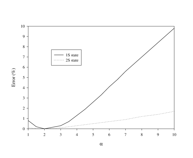
Figure 1: Evolution of the errors introduced by Eq. (54) as a function of $\alpha$ for the ground state and the first radial excitation.

where $\epsilon$ is a solution of a dimensionless Schrödinger equation. Since the BSQ approach gives the correct dimensional factor, the error depends only on $\alpha$ and $n$. Fig. 1 shows the evolution of errors with $\alpha$ for $n=1$ and $n=2$. For the ground states the errors are about $1\%$ (or smaller) for $\alpha\leq 4$. As expected, the errors decrease rapidly with the increase of the radial quantum number.

In general it is not obvious to understand why the formula (54) works so well since the exact solution is not known. For the harmonic oscillator case this formula gives the correct position of the energy levels. But it is more instructive to consider the case of a linear potential. Indeed, for $\alpha=1$ Eq. (54) leads to

$$\epsilon=\left(\frac{3\pi}{4}(n+3/4)\right)^{2/3}\equiv z^{2/3}.$$ (56)

This expression is just the leading term of an expansion ($z\gg 1$) for the values of the zeros of the Airy function (abra70, , p. 450). The exact solution is obtained by the summation of all the terms present in the expansion. In this particular case we can see how the Eq. (54) approximates the exact solution and how evolves this approximation. The formula (56) gives much better results than variational methods using trial wave functions for which the accuracy decrease rapidly as a function of $n$ (see for example (flam86, , p. 267)).

It is worth noting that a 3-dimensional calculation using BSQ approach introduces smaller errors than the 1-dimensional formulae obtained here. For example, for a linear potential the error is about $0.5\%$ for the ground state when a 3-dimensional calculation is performed, and about $0.75\%$ with the 1-dimensional formula. But in general the 3-dimensional calculations do not lead to analytical formulae or lead to complicated ones.

We can also calculate the mean square radius for a power-law potential. Using the definition (15) we can write:

$$\langle r^{2}\rangle=\left(\frac{1}{2a\mu}\right)^{2/(\alpha+2)}\,\frac{B(3/\alpha,1/2)}{B(1/\alpha,1/2)}\,\left(\frac{\alpha\pi}{B(1/\alpha,3/2)}\ (n+3/4)\right)^{4/(\alpha+2)}.$$ (57)

The calculation of the values of the wave functions at the origin leads to

$$|\Psi(0)|^{2}=\frac{\mu\alpha\,a^{1/\alpha}}{\pi B(1/\alpha,1/2)}\ E^{(\alpha-1)/\alpha},$$ (58)

but this time with the expression (54) for the energy. The evolution of the accuracy of formulae (57) and (58) with $\alpha$ and $n$ is similar to that shown in Fig. 1 for the energy.

The formula for the ratio of the wave function at the origin is given by

$$\left|\frac{\Psi_{m}(0)}{\Psi_{n}(0)}\right|^{2}=\left(\frac{m+3/4}{n+3/4}\right)^{2(\alpha-1)/(\alpha+2)}.$$ (59)

Some connection with previous general results can be done. If we suppose that $m=2$ and $n=1$, formula (59) shows that the ratio is greater than 1 if $\alpha>1$ $(d^{2}V(r)/dr^{2}>0)$ and smaller than 1 if $\alpha<1$ $(d^{2}V(r)/dr^{2}<0)$. This behavior is predicted by a general result obtained in Ref. mart77 . Eq. (54) shows that the energy behaves with the reduced mass as $E\propto\mu^{-\alpha/(\alpha+2)}$. Thus we can calculate that

$$\frac{d}{d\mu}\left(\frac{|\Psi_{n}(0)|^{2}}{\mu}\right)\propto\frac{1-\alpha}{\alpha+2}\,\mu^{-(1+2\alpha)/(\alpha+2)}.$$ (60)

This quantity is positive if $\alpha<1$ $(d^{2}V(r)/dr^{2}<0$ and $dV(r)/dr\geq 0)$ and negative if $\alpha>1$. This property is proved for $n=1$ in Ref. rosn78 .

The same calculations, for the energy and the r.m.s. radius, can be done for a semirelativistic kinematics but unfortunately they lead to complicated equations involving hypergeometric functions. The relativistic version of Eq. (54) can only be solved explicitly for the energy when one considers asymptotic behaviors. Thus further information about the observables cannot be extracted within the frame of a 1-dimensional semirelativistic approach.

To conclude this Section, we show that the 1-dimensional BSQ approach can also be used to derive a simple formula giving the number of $\ell=0$ bound states (a generalization to $\ell\not=0$ states can easily be done). We consider an attractive potential which vanishes at infinity (for example a Gaussian or a Yukawa potential). We calculate the value of the radial quantum number $n$ for $E=0$:

$$n=\frac{2\sqrt{2\mu}}{\pi}\int_{0}^{\infty}\sqrt{-V(r)}\,dr-\frac{1}{2}.$$ (61)

In general this number is not an integer except if the energy level $E=0$ is a real solution. But the integer part of $n$ gives the radial quantum number $n_{max}$ of the highest energy level. The formula for the number of bound states, $N=n_{max}+1$, of a given potential reads

$$N=\left[\frac{2\sqrt{2\mu}}{\pi}\int_{0}^{\infty}\sqrt{-V(r)}\,dr+\frac{1}{2}\right],$$ (62)

where $[x]$ denotes the integer part of $x$. For example, if $V(r)$ is of the form $V(r)=-af(br)$, we have

$$N=\left[\frac{2\sqrt{2\mu a}}{\pi b}\int_{0}^{\infty}\sqrt{f(y)}\,dy+\frac{1}{2}\right].$$ (63)

The remaining integral is a pure number and we can see immediately the dependence of the number of bound states on the potential parameters.

The same calculation can be performed in the semirelativistic case and we find

$$N=\left[\frac{1}{\pi}\int_{0}^{\infty}\sqrt{V(r)^{2}-4mV(r)}\,dr+\frac{1}{2}\right].$$ (64)

In this case the simple reduction performed in Eq. (63) cannot be obtained.

IV Summary

We have shown in this paper that the Bohr-Sommerfeld quantization procedure is an accurate and powerful method. It makes possible the derivation of reliable analytical formulae, from which one can easily study, e.g., the dependence of some physical quantities on the quantum numbers. Our study emphasizes the strong connection existing between the Regge and radial trajectories for the energy within a potential model, which could play an important role in elucidating the confining properties of the quark-antiquark interaction when additional experimental information is obtained on the radial excitations of light mesons; the study of other observables (decay widths, mean square radii, electromagnetic mass splittings,…) could put supplementary constraints on this interaction.

We have also shown that even if semirelativistic calculations yield results quantitatively different compared with nonrelativistic calculations some common general features of observables are observed. The asymptotic behavior of orbital and radial trajectories, for the energy and the r.m.s. radius, are the same for a potential which behaves asymptotically as a power-law. Moreover the ratio of the slopes of these trajectories depends only on the value of the power of the confining potential.

At last, we have shown in Sec. II.3 that 1-dimensional calculations lead to very simple approximated formula for the energy, the r.m.s. radius and the wave function at the origin in the $\ell=0$ sector. We have also obtained formulae which give the number of bound states of a given potential for the nonrelativistic and semirelativistic case.

Of course, a BSQ approach cannot replace a correct quantum description since it is only an approximate method which is not completely self-consistent. For example, we need to use the Schrödinger equation to give a definition of the wave function at the origin to be able to calculate this quantity with this formalism. Moreover some quantum concepts have no meaning in this framework. But we emphasize that for some cases the evaluation of observables (evaluation of average values) can be performed using this old method; even if calculations yield complicated formulae it is often possible to extract interesting information from an analytical relation and in this way guide full quantum calculations.

Table 1: Energies, r.m.s. radii and wave functions at the origin for a selected set of mesons, obtained from the Schrödinger equation and from the BSQ approximation for the Cornell potential, using the parameters of Ref. fulc94 (masses are given in MeV, r.m.s. radii in GeV^-1, and wave functions at the origin in GeV³).

States	Exact Masses	BSQ	Exact $\sqrt{\bar{r}^{2}}$	BSQ	Exact $|\Psi(0)|^{2}$	BSQ
$n\bar{n}$ states
$1S$	681	681	4.04	3.97	7.5715 10-3	7.6383 10-3
$2S$	1577	1577	7.32	7.30	6.7084 10-3	6.7601 10-3
$1P$	1240	1242	5.82	5.79
$1D$	1692	1693	7.32	7.31
$n\bar{s}$ states
$1S$	794	794	3.65	3.58	1.0653 10-2	1.0784 10-2
$2S$	1626	1626	6.68	6.65	9.2169 10-3	9.3099 10-3
$1P$	1320	1321	5.30	5.28
$1D$	1738	1739	6.69	6.67
$s\bar{s}$ states
$1S$	1004	1002	3.17	3.10	1.7346 10-2	1.7668 10-2
$2S$	1759	1758	5.87	5.85	1.4416 10-2	1.4623 10-2
$1P$	1490	1492	4.67	4.65
$1D$	1869	1870	5.91	5.90
$n\bar{c}$ states
$1S$	1973	1972	3.36	3.29	1.4194 10-2	1.4418 10-2
$2S$	2757	2757	6.19	6.17	1.2004 10-2	1.2154 10-2
$1P$	2474	2475	4.92	4.89
$2P$	3125	3126	7.43	7.42
$c\bar{c}$ states
$1S$	3067	3062	2.26	2.19	5.8025 10-2	6.0210 10-2
$2S$	3693	3691	4.38	4.36	4.2153 10-2	4.3351 10-2
$1P$	3497	3497	3.48	3.46
$2P$	3991	3991	5.35	5.34
$1D$	3806	3806	4.47	4.46
$2D$	4242	4242	6.17	6.17
$n\bar{b}$ states
$1S$	5313	5311	3.16	3.09	1.7607 10-2	1.7937 10-2
$2S$	6066	6065	5.85	5.83	1.4613 10-2	1.4825 10-2
$1P$	5799	5800	4.65	4.63
$2P$	6420	6420	7.04	7.03
$b\bar{b}$ states
$1S$	9448	9439	1.13	1.04	7.3583 10-1	7.7015 10-1
$2S$	10007	10003	2.55	2.52	3.3903 10-1	3.5597 10-1
$1P$	9901	9900	2.04	2.02
$2P$	10261	10261	3.28	3.28
$1D$	10148	10148	2.74	2.73

Table 2: Energies and r.m.s. radii for a selected set of mesons, obtained from the spinless Salpeter equation and from the BSQ approximation for the Cornell potential, using the parameters of Ref. fulc94 (masses are given in MeV and r.m.s. radii in GeV^-1).

States	Exact Masses	BSQ	Exact $\sqrt{\bar{r}^{2}}$	BSQ
$n\bar{n}$ states
$1S$	703	683	3.30	3.22
$2S$	1416	1413	5.40	5.39
$1P$	1240	1236	4.62	4.60
$1D$	1642	1639	5.60	5.60
$s\bar{s}$ states
$1S$	1004	991	2.96	2.87
$2S$	1695	1691	5.04	5.02
$1P$	1508	1506	4.27	4.25
$1D$	1885	1884	5.27	5.26
$c\bar{c}$ states
$1S$	3067	3056	2.05	1.97
$2S$	3668	3662	3.89	3.85
$1P$	3504	3504	3.19	3.18
$2P$	3970	3970	4.76	4.76
$1D$	3811	3811	4.07	4.06
$2D$	4216	4216	5.48	5.48
$b\bar{b}$ states
$1S$	9448	9433	1.10	1.01
$2S$	9999	9993	2.45	2.42
$1P$	9900	9900	1.99	1.98
$2P$	10262	10262	3.17	3.17
$1D$	10150	10150	2.66	2.66