Gereralized Parton Distributions:
Analysis and Applications

Abstract

Results from a recent analysis of the zero-skewness generalized parton distributions (GPDs) for valence quarks are discussed. The analysis bases on a physically motivated parameterization of the GPDs with a few free parameters adjusted to the available nucleon form factor data. Various moments of the GPDs as well as their Fourier transfroms, the quark densities in the impact parameter plane, are also presented. The $1/x$ moments of the zero-skewness GPDs are form factors specific to Compton scattering off protons within the handbag approach. The results of the GPD analysis enables one to predict Compton scattering.
Talk presented at the workshop on Lepton Scattering and the Structure of Hadrons and Nuclei, Erice Italy) September 2004

1 Factorization and general parton distributions

In recent years we learned how to deal with hard exclusive reactions within QCD. In analogy to hard inclusive reactions like deep inelastic lepton-nucleon scattering (DIS), the process amplitudes factorize in partonic subprocess amplitudes, calculable in perturbation theory, and in GPDs which parameterize soft hadronic matrix elements. In some cases rigorous proofs of factorization exist. For other processes factorization is shown to hold in certain limits or under certain assumptions or is just a hypothesis.

The GPDs which are defined by Fourier transforms of bilocal proton matrix elements of quark field operators [1], describe the emission and reabsorption of partons by the proton carrying different momentum fractions $x_{1}$ and $x_{2}$, respectively. Usually the GPDs are parameterized in terms of the momentum transfer from the initial to the final proton, $t$, the average momentum fraction $x$ and the skewness, $\xi$. The latter variables are related to the individual momentum fractions $x_{1}$ and $x_{2}$ by

$$x_{1}\,=\,\frac{x+\xi}{1+\xi}\,,\qquad x_{2}\,=\,\frac{x-\xi}{1-\xi}\,.$$ (1)

Although the GPDs are not calculable with a sufficient degree of accuracy at present, we know many of their properties. Thus, for instance, they satisfy the reduction formulas

$$H^{q}(x,\xi=0,t=0)\,=\,q(x)\,,\qquad\widetilde{H}^{q}(x,\xi=0,t=0)\,=\,\Delta q(x)\,,$$ (2)

i.e. in the forward limit of zero momentum transfer and zero skewness, two of them, namely $H$ and $\widetilde{H}$ reduce to the usual unpolarized and polarized parton distributions (PDFs), respectively. The other two GPDs, $E$ and $\widetilde{E}$, are not accessible in DIS. Another property of the GPDs is the polynomiality which comes about as a consequence of Lorentz covariance

$$\int^{1}_{-1}\,dx\,x^{n-1}\,H^{q}(x,\xi,t)\,=\,\sum^{[n/2]}_{i=0}\,h^{q}_{n,i}(t)\,\xi^{i}\,,$$ (3)

where $[n/2]$ denotes the largest integer smaller than or equal to $n/2$. Eq. (3) holds analogously for the other GPDs and, for $n=1$ implies sum rules for the form factors of the nucleon, e.g.

$$F^{q}_{1}(t)\,=\,h^{q}_{1,0}(t)\,=\,\int^{1}_{-1}\,dxH^{q}(x,\xi,t)\,.$$ (4)

Reinterpreting as usual a parton with a negative momentum fraction $x$ as a antiparton with positive $x$ ($H^{\bar{q}}(x)=-H^{q}(-x)$), one becomes aware that this sum rules provides the difference of the contributions from quarks and antiquarks of given flavor to the Dirac form factor of the nucleon. Introducing the combination

$$H^{q}_{v}(x,\xi,t)\,=\,H^{q}(x,\xi,t)-H^{\bar{q}}(x,\xi,t)\,,$$ (5)

which, in the forward limit, reduces to the usual valence quark density $q_{v}(x)=q(x)-\bar{q}(x)$, one finds for the Dirac form factor the representation

$$F_{1}^{p(n)}(t)\,=\,e_{u(d)}\int_{0}^{1}\,dx\,H_{v}^{u}(x,\xi,t)+e_{d(u)}\int_{0}^{1}\,dx\,H_{v}^{d}(x,\xi,t)\,.$$ (6)

Here, $e_{q}$ is the charge of the quark $q$ in units of the positron charge. There might be contributions from other quarks, $s,c,...$, to the sum rule (6). These possible contributions are likely small ( in the forward limit one has for instance $s(x)\simeq\bar{s}(x)$ [2]) and neglected in the sum rule (6). A representation anlogue to (6) holds for the Pauli form factor replacing $H$ by $E$.

The isovector axial vector form factor, on the other hand, satisfies the following sum rule

$$F_{A}(t)\,=\,\int_{0}^{1}dx\,\Big{[}\widetilde{H}^{u}(x,\xi,t)-\widetilde{H}^{d}(x,\xi,t)\Big{]}+2\int_{0}^{1}dx\,\Big{[}\widetilde{H}^{\bar{u}}(x,\xi,t)-\widetilde{H}^{\bar{d}}(x,\xi,t)\Big{]}\,,$$ (7)

where $\widetilde{H}^{\bar{q}}(x)=\widetilde{H}^{q}(-x)$. At least for small $t$ the magnitude of the second integral in Eq. (7) reflects the size of the flavor-singlet combination $\Delta\bar{u}(x)-\Delta\bar{d}(x)$ of forward densities. This difference is poorly known, and at present there is no experimental evidence that it might be large [3]. In the analysis of the polarized PDFs performed by Blümlein and Böttcher Ref. [4] it is even zero. In a perhaps crude approximation the second term in (7) can be neglected.

We also know how the GPDs evolve with the scale. They satisfy positivity bounds and possess overlap representations. But, I repeat, we don’t know how to calculate them accurately from QCD at present. Thus, we have either to rely on models or we have to extract the GPDs from experiment as it has been done for the PDFs, see for instance Refs. [2, 4]. The universality property of the GPDs, i.e. their process independence, subsequently allows to predict other hard exclusive reactions once the GPDs have been determined in the analysis of a given process. This way QCD acquires a predictive power for hard processes provided factorization holds.

2 Analysis of the zero-skewness GPDs

At present the data basis is too sparse to allow for a phenomenological extraction of the GPDs as a function of the three variables $x$, $t$ and $\xi$. Lacking are in particular sufficient data on deeply virtual Compton scattering. Available is, on the other hand, a fair amount of nucleon form factor data, spread over a fairly large range of momentum transfer, see references given in [5, 6]. More form factor data will become available in the near future.

The form factors represent the first moment of GPDs for any value of the skewness and, in particular, at $\xi=0$, see (6), (7). Mathematically one needs infinitely many moments to deduce the integrand, i.e. the GPDs. However, from phenomenological experience with particle physics one can expect the GPDs to be rather smooth functions and, therefore, a small number of moments may suffer to fix the GPDs. A first attempt in this direction adopts the extreme (and at present the only feasible) point of view that the lowest moment of a GPD suffices to determime it [6] (see also Ref. [7]). Indeed using recent results on PDFs [2, 4] and form factor data [5] as well as suitable, physically motivated parameterizations of the GPDs with a few parameters adjusted to data, one can indeed carry through this analysis. Needless to say that this method while phenomenologically succesful as I will discuss below, does not lead to a unique result. Other parameterizations which may imply different physics, cannot be excluded in the present stage of the GPD analysis. In principle this can be remedied by the inclusion of higher order moments from lattice QCD. Provided the lattice results are obtained in a scenario with light quarks or reliably extrapolated to the chiral limit, a combined analysis of form factor and lattice data will lead to improved results on the GPDs with a lesser or even no dependence on the chosen parameterization. The analysis advocated for in Ref. [6] can easily accomodate higher order moments. The LHPC [8] and QCDSF [9] collaborations have recently presented results on GPD moments in scenarios with pion masses around $800\,~{}{\rm MeV}$. These results have not used in the analysis presented in Ref. [6] for obvious reasons but they indicate that, in a few years, the quality of the lattice results may suffice for use in a GPD analysis.

In Ref. [6] $\xi=0$ is chosen (implying $x_{1}=x_{2}$) and a parameterization of the GPDs is exploited that combines the usual PDFs with an exponential $t$ dependence (the argument $\xi=0$ is dropped in the following for convenience)

$$H_{v}^{q}(x,t)\,=\,q_{v}(x)\exp[tf_{q}(x)]\,,$$ (8)

where the profile function reads

$$f_{q}(x)\,=\,\big{[}\alpha^{\prime}\,\log(1/x)+B_{q}\big{]}(1-x)^{n+1}+A_{q}x(1-x)^{n}\,.$$ (9)

This ansatz is motivated by the expected Regge behaviour at low $t$ and low $x$ [10] (where $\alpha^{\prime}$ is the Regge slope for which the value $0.9\,~{}{\rm GeV}^{2}$ is imposed). For large $t$ and large $x$, on the other hand, one expects a behaviour like $f_{q}\sim 1-x$ from the overlap model [11, 12, 13, 14]. The ansatz (8), (9) interpolates between the two limits smoothly  and allows the generalization to the case $n=2$. The ansatz (8), (9) matches the following criteria for a reasonable parameterization

• simplicity

• consistency with theoretical and phenomenological constraints

• plausible interpretation of the parameters (if possible)

• stability with respect to variations of PDFs

• stability under evolution (scale dependence of GPDs can be absorbed into parameters)

A fit of the ansatz (8), (9) to the data on the Dirac form factor ranging from $t=0$ up to $\simeq 30\,~{}{\rm GeV}^{2}$, exploiting the sum rule (6) and using the CTEQ PDFs [2], leads to very good results with the three parameters

$$B_{u}\,=\,B_{d}\,=\,(0.59\pm 0.03)\,~{}{\rm GeV}^{-2}\,,\quad A_{u}\,=\,(1.22\pm 0.020)\,~{}{\rm GeV}^{-2}\quad A_{d}\,=\,(2.59\pm 0.29)\,~{}{\rm GeV}^{-2}\,,$$ (10)

quoted for the case $n=2$ and at a scale of $\mu=2\,~{}{\rm GeV}$.

In Fig. 1 the results for $H$ are shown at two values of $t$. While at small $t$ the behaviour of the GPD still reflects that of the parton densities it exhibits a pronounced maximum at larger values of $t$. The maximum moves towards $x=1$ with increasing $t$ and becomes more pronounced. In other words only a limited range of $x$ contributes to the form factor substantially and this range moves with $t$ in parallel with the position of the maximum of $H$.

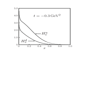
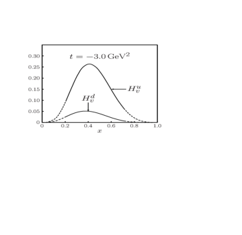
Figure 1: Result for the valence GPD $H_{v}^{q}(x,t)$ at the scale $\mu=2~{}{\rm GeV}$ and for $n=2$ obtained in the analysis presented in [6]. The dashed lines indicate regions of $x$ where only $5\%$ of the sum rule (6) is accumulated.

The quality of the fit is very similar in both the cases, $n=1$ and 2; the results for the GPDs and related quantities agree very well with each other. Substantial differences between the two results only occur for very low and very large values of $x$, i.e. in regions which are nearly insensitive to the form factor data. It is the physical interpretation of the results which favours the fit with $n=2$. Indeed the average distance between the struck quark and the cluster of spectators becomes unphysical large for $x\to 1$ in the case $n=1$; it grows like $\sim(1-x)^{-1}$ while, for $n=2$, it tends to a constant value of about 0.5 fm [6].

The analogue analysis of the axial and Pauli form factors, with parameterizations similar to Eqs. (8), (9), provides the GPDs $\widetilde{H}$ and $E$. They behave similar to $H$. Noteworthy differences are the opposite signs of $\widetilde{H}^{u}$ ($E^{u}$) and $\widetilde{H}^{d}$ ($E^{q}$) and the approximately same magnitude of $E^{u}$ and $E^{d}$ at least for not too large values of $t$. For $H^{q}$ and $\widetilde{H}^{q}$, on the other hand, the $d$-quark contributions are substantially smaller in magnitude than the $u$-quark ones, see Fig. 1. Since there is no data available for the pseudoscalar form factor of the nucleon the GPD $\widetilde{E}$ cannot be determined this way.

I repeat the results for the GPDs are not unique. An alternative ansatz is for instance

$$H_{v}^{q}(x,t)\,=\,q_{v}(x)\Big{[}1-tf_{q}(x)/p\Big{]}^{-p}\,.$$ (11)

Although reasonable fits to the form factors are obtained with it for $p\raisebox{-4.0pt}{$\,\stackrel{{\scriptstyle\textstyle>}}{{\sim}}\,$}2.5$ it is physically less appealing than (8): the combination of Regge behaviour at small $x$ and $t$ with the dynamics of the Feynman mechanism is lost. The resulting GPDs have a broader shape and $H(x=0,t)$ remains finite. Thus, small $x$ also contribute to the high-$t$ form factors for the ansatz (11).

3 Moments and interpretation

Having the zero-skewness GPDs at disposal one can evaluate various moments, some of them are displayed in Fig. 2. Comparison with recent results from lattice QCD [8, 9] reveals remarkable agreement of their $t$ dependencies given the uncertainties in the GPD analysis [6] and in the lattice calculations [8, 9].

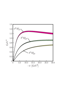
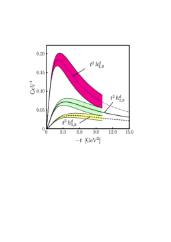
Figure 2: The first three moments of valence GPDs $H_{v}^{u}$ (left) and $H_{v}^{d}$ (right), scaled with $t^{2}$. The error bands denote the parametric uncertainty resulting from the fit to the Dirac form factors $F_{1}^{p}$ and $F_{1}^{n}$.

An interesting property of the moments is that the $u$ and $d$ quark contributions drop with different powers of $t$. These powers are determined by the large-$x$ behaviour of $q_{v}$ and $f_{q}$, namely

$$q_{v}\sim(1-x)^{\beta_{q}}\,,\qquad f_{q}\sim(1-x)^{2}\,,$$ (12)

where $\beta_{u}\simeq 3.4$ and $\beta_{d}\simeq 5$ [2]. Because of the pronounced maximum the GPDs exhibits, see Fig. 1, the sum rule (6) can be evaluated in the saddle point approximation. For large t this leads to

$$h^{q}_{1,0}\sim|t|^{-(1+\beta_{q})/n}\,.$$ (13)

With the CTEQ values for $\beta_{q}$ one obtains a drop of the form factor $F_{1v}^{u}$ slightly faster than $t^{-2}$ while the $d$-quark form factor falls as $t^{-3}$. Strengthened by the charge factor the $u$-quark contribution dominates the proton’s Dirac form factor for $t$ larger than about $5\,~{}{\rm GeV}^{2}$, the $d$-quark contribution amounts to less than $10\%$. High quality neutron form factor data above $3\,~{}{\rm GeV}^{2}$ would allow for a direct examination of the different powers. The power behaviour bears resemblance to the Drell-Yan relation [15]. In fact the common underlying dynamics is the Feynman mechanism . The Drell-Yan relation is, however, an asymptotic result ($x\to 1$, $t\to\infty$) which bases on the assumption of valence Fock state dominance. In the GPD analysis Eq. (13) holds provided the saddle point lies in the region where the bulk of the contribution to the Dirac form factor is accumulated.

A combination of the second moments of $H$ and $E$ at $t=0$ is Ji’s sum rule [16] which allows for an evaluation of the valence quark contribution to the orbital angular momentum the quarks inside the proton carry

$$\langle L_{v}^{q}\rangle\,=\,\frac{1}{2}\,\int_{0}^{1}dx\Big{[}xE_{v}^{q}(x,t=0)+xq_{v}(x)-\Delta q_{v}(x)\Big{]}\,.$$ (14)

A value of -0.08 has been found in Ref. [6] at the scale $\mu=2\,~{}{\rm GeV}$ for the average valence quark contribution to the orbital angular momentum.

In contrast to the parton distributions which only provide information on the longitudinal distribution of quarks inside the nucleon, GPDs also give access to the transverse structure of the nucleon by Fourier transforming the GPD with respect to $\sqrt{-t}$. As shown by Burkardt [17], a density interpretation of the zero-skewness GPDs is obtained in the mixed representation of longitudinal and transverse position in the infinite-momentum frame. In particular

$$q_{v}(x,{\bf b})\,=\,\int\frac{d^{2}{\bf\Delta}}{(2\pi)^{2}}\,e^{-i{\bf b}\cdot{\bf\Delta}}\,H_{v}^{q}(x,t=-\Delta^{2})\,,$$ (15)

gives the probability to find a valence quark with longitudinal momentum fraction $x$ and impact parameter ${\bf b}$. Together with the analogue Fourier transform of $E_{v}^{q}(x,t)$ one can form the combination ($m$ being the mass of the proton)

$$q_{v}^{X}(x,{\bf b})\,=\,q_{v}(x,{\bf b})-\frac{\;b^{Y}}{m}\,\frac{\partial}{\partial{\bf b}^{2}}\,e_{v}^{q}(x,{\bf b})\,,$$ (16)

which gives the probability to find an unpolarized valence quark with momentum fraction $x$ and impact parameter ${\bf b}=(b^{X},b^{Y})$ in a proton that moves rapidly along the $Z$ direction and is polarized along the $X$ direction [17]. In Fig. 3 the results for the GPDs are shown as tomography plots in the impact parameter space for fixed momentum fractions. For small $x$ one observes a very broad distribution while, at large $x$, it becomes more focussed on the center of momentum defined by $\sum_{i}x_{i}{\bf b}_{i}=0$ ($\sum_{i}x_{i}=1$). In a proton that is polarized in the $X$ direction the symmetry around the $Z$ axis is lost and the center of the density is shifted in the $Y$ direction away from the center of momentum, downward for $d$ quarks and upward for $u$ ones. Thus, a polarization of the proton induces a flavor segregation in the direction orthogonal to the direction of the polarization and the proton momentum.

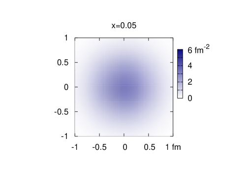
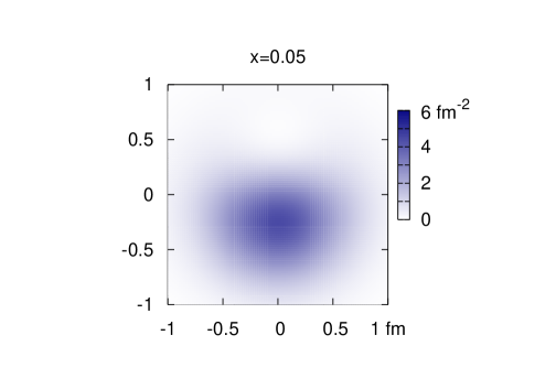
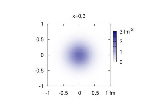
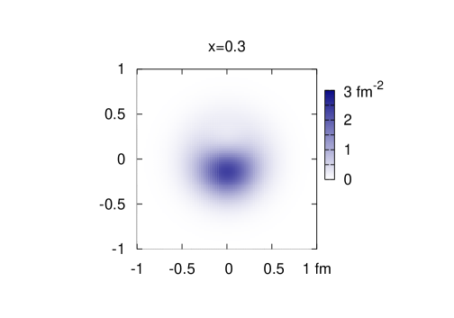
Figure 3: Tomography plots of $d_{v}(x,{\bf b})$ (left) and $d_{v}^{X}(x,{\bf b})$ (right) in the transverse $b^{X}$–$b^{Y}$ plane (in units of fm). The longitudinal momentum fraction $x$ is fixed to $0.05$ (top) and $0.3$ (bottom). The scale of intensity is given on the right hand side of the plots.

4 Applications: Compton scattering and photoproduction

As I discussed in the preceeding sections the analysis of the GPDs gives insight in the transverse distribution of quarks inside the proton. However, there is more in it. With the $\xi=0$ GPDs at hand one can now predict hard wide-angle exclusive reactions like Compton scattering off protons or meson photo- and electroproduction . For these reactions one can work in a symmetrical frame where skewness is zero. A symmetrical frame is, for instance, a c.m.s. rotated in such a way that the initial and final protons have the same light-cone plus component. Hence, $\xi=0$. It has been argued [12, 14, 18] that, for large Mandelstam variables ($s,\;-t,\;-u\gg m^{2}$), the amplitudes for these processes factorize in a hard partonic subprocess, e.g. Compton scattering off quarks - see Fig. 4, and in form factors representing $1/x$-moments of zero-skewness GPDS. For Compton scattering these form factors read

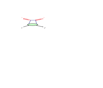
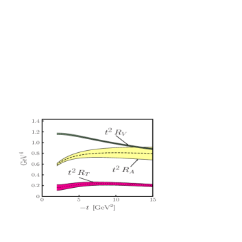
Figure 4: Handbag diagram for Compton scattering (left) and the Compton form factors, scaled by $t^{2}$, evaluated from the GPDs determined in [6] (right). The bands represent the parametric uncertainties of the form factors [6].

$$R_{V}(t) \simeq \sum_{q}e_{q}^{2}\int_{0}^{1}\frac{dx}{x}\,H^{q}_{v}(x,t)\,,$$

$$R_{A}(t) \simeq \sum_{q}e_{q}^{2}\int_{0}^{1}\frac{dx}{x}\,\widetilde{H}^{q}_{v}(x,t)\,,$$

$$R_{T}(t) \simeq \sum_{q}e_{q}^{2}\int_{0}^{1}\frac{dx}{x}\,E^{q}_{v}(x,t)\,.$$ (17)

These relations only hold approximately even though with a very high degree of accuracy at large $t$ since contributions from sea quarks can safely be neglected . A pseudoscalar form factor related to the GPD $\widetilde{E}$, decouples in the symmentric frame. Numerical results for the Compton form factors are shown in Fig. 4. Approximately the form factors $R_{i}$ behave $\sim t^{-2}$. The particular flat behaviour of the scaled form factor $t^{2}R_{T}$ is a consequence of a cancellation between the $u$ and $d$-quark contributions. The ratio $R_{T}/R_{V}$ behaves differently from the corresponding ratio of their electromagnetic analogues $F_{2}$ and $F_{1}$.

The handbag contribution leads to the following leading-order result for the Compton cross section [12, 19]

$$\frac{d\sigma}{dt} = \frac{d\hat{\sigma}}{dt}\left\{\frac{1}{2}\,\Big{[}R_{V}^{2}(t)\,+\frac{-t}{4m^{2}}R_{T}^{2}(t)+R_{A}^{2}(t)\Big{]}\right.$$ (18)

$$\left.-\frac{us}{s^{2}+u^{2}}\,\Big{[}R_{V}^{2}(t)\,+\frac{-t}{4m^{2}}R_{T}^{2}(t)-R_{A}^{2}(t)\Big{]}\right\}\,,$$

where $d\hat{\sigma}/dt$ is the Klein-Nishina cross section for Compton scattering off massless, point-like spin-1/2 particles of charge unity. Next-to-leading order QCD corrections to the subprocess have been calculated in Ref. [19]. They are not displayed in (18) but taken into account in the numerical results discussed below. Another interesting observable in Compton scattering is the helicity correlation, $A_{LL}$, between the initial state photon and proton or, equivalently, the helicity transfer, $K_{LL}$, from the incoming photon to the outgoing proton. In the handbag approach one obtains [19]

$$A_{LL}\,=\,K_{LL}\simeq\frac{s^{2}-u^{2}}{s^{2}+u^{2}}\,\frac{R_{A}(t)}{R_{V}(t)}+O(\alpha_{s})\,,$$ (19)

where the factor in front of the form factors is the corresponding observable for $\gamma q\to\gamma q$. The result (19) is a robust prediction of the handbag mechanism, the magnitude of the subprocess helicity correlation, $\hat{A}_{LL}$, is only diluted somewhat by the ratio of the form factors $R_{A}$ and $R_{V}$. It is to be stressed that $A_{LL}$ and $K_{LL}$ are identically in the handbag approach because the quarks are assumed to be massless and consequently there is no quark helicity flip. For an alternative approach, see Ref. [20]. It is also important to keep in mind that both the results, (18) and (19), hold for $s,\;-t,\;-u\gg m^{2}$.

Inserting the Compton form factors (17) into Eqs. (18) and (19), one can predict the Compton cross section in the wide-angle region as well as the helicity correlation $A_{LL}=K_{LL}$. The results for sample values of $s$ are shown in Fig. 5. The inner bands of the predictions for $d\sigma/dt$ reflect the parametric errors of the form factors, essentially that of the vector form factor which dominates the cross section. The outer bands indicate estimates of the target mass corrections, see [21]. As a minimum condition to the kinematical approximations made in the handbag approach, predictions are only shown for $-t$ and $-u$ larger than about $2.4\,~{}{\rm GeV}^{2}$. The JLab E99-114 collaboration [22] will provide accurate cross section data soon which will allow for a crucial examination of the predictions from the handbag mechanism.

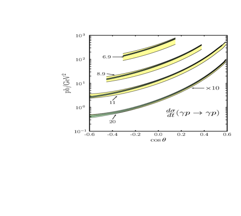
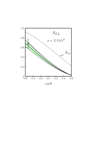
Figure 5: The unpolarized cross section (left) and the helicity correlation parameter $A_{LL}$ (right) for wide-angle Compton scattering as functions of the c.m.s. scattering angle $\theta$. The cross section is shown at $s=6.9,8.9,11$ and $20~{}{\rm GeV}^{2}$, the latter cross section is multiplied by 10. The helicity correlation is presented at $s=11\,~{}{\rm GeV}^{2}$ (solid line with error band). The dashed line is the prediciton at $s=20\,~{}{\rm GeV}^{2}$ and $\hat{A}_{LL}$ is the result for Compton scattering off quarks. The data point [23] is measured at $s=6.9\,~{}{\rm GeV}^{2}$. Both observables are evaluated at NLO QCD with the Compton form factors shown in Fig. 4. The error bands are explained in the text.

The JLab Hall A collaboration [23] has presented a first measurement of $K_{LL}$ at $s=6.9\,~{}{\rm GeV}^{2}$ and $t=-4\,~{}{\rm GeV}^{2}$. The kinematical requirement of the handbag mechanism, $s,\;-t,\;-u\gg m^{2}$, is not satisfied for this measurement since $-u$ is only $1.13\,~{}{\rm GeV}^{2}$. One therefore has to be very cautious when comparing this experimental result with the handbag predictions, there might be large dynamical and kinematical corrections. Nevertheless the agreement of this data point with the prediction from the handbag at $s=11\,~{}{\rm GeV}^{2}$ is, with regard to the mild energy dependence of $K_{LL}$ in (19), a non-trivial and promising fact. Polarization data at higher energies are desired as well as a measurement of the angle dependence. The Jlab Hall A collaboration [23] has also measured the polarization transfer $K_{LS}$ from a longitudinally polarized incident photon to the sideway polarization of the outgoing proton. In Ref. [23] a value of $0.114\pm 0.078\pm 0.04$ is obtained for it at the same kinematics as for $K_{LL}$ while we found $0.10\pm 0.02$ at this admittedly small energy.

The handbag approach also applies to wide-angle photo- and electroproduction of pseudoscalar and vector mesons. The amplitudes again factorize into a parton-level subprocess, $\gamma q\to Mq$, and form factors which represent $1/x$-moments of GPDs [18]. Their flavor decomposition differs from those appearing in Compton scattering, see (17). Here, it reflects the valence quark structure of the produced meson. Since the GPDs and, hence, the form factors for a given flavor, $R_{i}^{q}$, $i=V,A,T$ are process independent they are known from the analysis of Ref. [6] for $u$ and $d$ quarks (if the contributions from sea quarks can be ignored). Therefore, the soft physics input to calculations of photo-and electroproduction of pions and $\rho$ mesons within the handbag approach is now known.

One may also consider the time-like process $\gamma\gamma\leftrightarrow p\bar{p}$ in the handbag approach [24]. Similar form factors as in the space-like region occur which are now functions of $s$ and represent moments of the $p\bar{p}$ distribution amplitudes, time-like versions of GPDs. With sufficient form factor data at disposal one may attempt a determination of the time-like GPDs.

5 Summary

Results from a first analysis of GPDs at zero skewness have been discussed. The analysis, performed in analogy to those of the usual parton distributions, bases on a physically motivated parameterization of the GPDs with a few free parameters fitted to the available nucleon form factor data. The analysis of the form factors provides results on the valence-quark GPDs $H$, $\widetilde{H}$ and $E$. Interesting results on the structure of the nucleon, in particular on the distribution of the quarks in the plane transverse to the direction of the nucleon’s momentum are obtained. One finds that a polarization of the nucleon induces a flavor separation in the direction orthogonal to the those of the momentum and of the polarization. An estimate of the average orbital angular momentum the valence quarks carry lead to a value of $-0.08$.

The zero skewness GPDs are the soft physics input to hard wide-angle exclusive reactions. For Compton scattering, for instance, the soft physics is encoded in specific form factors which represent $1/x$ moments of zero-skewness GPDs. Using the results from the GPD analysis to evaluate these form factors, one can give interesting predictions for the differential cross section and helicity correlations in Compton scattering. These predicitons still await their experimental examination.

References

- [1] D. Müller, D. Robaschik, B. Geyer, F. M. Dittes and J. Hořejši, Fortsch. Phys. 42 (1994) 101 [hep-ph/9812448]; A. V. Radyushkin, Phys. Rev. D 56 (1997) 5524 [hep-ph/9704207]; X. Ji, Phys. Rev. D 55 (1997) 7114 [hep-ph/9609381].
- [2] J. Pumplin et al [CTEQ collaboration], JHEP 0207 (2002) 012 [hep-ph/0201195].
- [3] A. Airapetian et al. [HERMES Collaboration], Phys. Rev. Lett. 92 (2004) 012005 [hep-ex/0307064].
- [4] J. Blümlein and H. Böttcher, Nucl. Phys. B 636 (2002) 225 [hep-ph/0203155].
- [5] E.J. Brash et al, Phys. Rev. C 65 (2002) 051001 [hep-ex/0111038].
- [6] M. Diehl, T. Feldmann, R. Jakob and P. Kroll, hep-ph/0408173, to be published in Eur. Phys. J..
- [7] M. Guidal, M. V. Polyakov, A. V. Radyushkin and M. Vanderhaeghen, hep-ph/0410251.
- [8] P. Hägler, J. W. Negele, D. B. Renner, W. Schroers, T. Lippert and K. Schilling [LHPC Collaboration], hep-ph/0410017.
- [9] M. Göckeler et al. [QCDSF Collaboration], hep-lat/0410023.
- [10] H.D.I. Arbarbanel, M.L. Goldberger and S.B. Treiman, Phys. Rev. Lett. 22 (1969) 500 ; P.V. Landshoff, J.C. Polkinghorne and R.D. Short, Nucl. Phys. B 28 (1971) 225 ; M. Penttinen, M. V. Polyakov and K. Goeke, Phys. Rev. D 62 (2000) 014024 [hep-ph/9909489].
- [11] V. Barone et al., Z. Phys. C 58 (1993) 541 ; J. Bolz and P. Kroll, Z. Phys. A 356 (1996) 327 [hep-ph/9603289].
- [12] M. Diehl, T. Feldmann, R. Jakob and P. Kroll, Eur. Phys. J. C 8 (1999) 409 [hep-ph/9811253].
- [13] M. Diehl, T. Feldmann, R. Jakob, and P. Kroll, Nucl. Phys. B 596 (2001) 33 , Erratum-ibid. 6056472001, [hep-ph/0009255].
- [14] A. V. Radyushkin, Phys. Rev. D 58 (1998) 114008 [hep-ph/9803316].
- [15] S. D. Drell and T. M. Yan, Phys. Rev. Lett. 24 (1970) 181 .
- [16] X.-D. Ji, Phys. Rev. Lett. 78 (1997) 610 [hep-ph/9603249].
- [17] M. Burkardt, Phys. Rev. D 62 (2000) 071503 , Erratum-ibid. 661199032002, [hep-ph/0005108], Int. J. Mod. Phys. A 18 (2003) 173 [hep-ph/0207047].
- [18] H. W. Huang and P. Kroll, Eur. Phys. J. C 17 (2000) 423 [hep-ph/0005318]; H. W. Huang, R. Jakob, P. Kroll and K. Passek-Kumericki, Eur. Phys. J. C 33 (2004) 91 [hep-ph/0309071].
- [19] H. W. Huang, P. Kroll and T. Morii, Eur. Phys. J. C 23 (2002) 301 [Erratum-ibid. C 31, 279 (2003)] [hep-ph/0110208].
- [20] G. A. Miller, Phys. Rev. C 69, 052201 (2004) [nucl-th/0402092].
- [21] M. Diehl et al., Phys. Rev. D 67 (2003) 037502 [hep-ph/0212138].
- [22] E99-114 JLab collaboration, spokespersons C. Hyde-Wright, A. Nathan and B. Wojtsekhowski.
- [23] D. J. Hamilton et al. [Jefferson Lab Hall A Collaboration], nucl-ex/0410001.
- [24] M. Diehl, P. Kroll and C. Vogt, Eur. Phys. J. C 26 (2003) 567 [hep-ph/0206288].