hep-ph/0412165
Dynamical Zero in
– Scattering and
the
Neutrino Magnetic Moment
J. Bernabéua, J. Papavassilioua, and M. Passeraa,b
a Departament de Física Teòrica and IFIC Centro Mixto,
Universitat de València–CSIC, E-46100, Burjassot, València,
Spain
b Dipartimento di Fisica “G. Galilei”, Università
di Padova and
INFN, Sezione di Padova, I-35131, Padova, Italy
Abstract
The Standard Model differential cross section for elastic scattering vanishes exactly, at lowest order, for forward electrons and incident energy close to the rest energy of the electron. This dynamical zero is not induced by a fundamental symmetry of the Lagrangian but by a destructive interference between the left- and right-handed chiral couplings of the electron in the charged and neutral current amplitudes. We show that lowest-order analyses based on this favorable kinematic configuration are only mildly affected by the inclusion of the radiative corrections in the differential cross section, thus providing an excellent opportunity for the search of “new physics”. In the light of these results, we discuss possible methods to improve the upper limits on the neutrino magnetic moment by selecting recoil electrons contained in a forward narrow cone. We conclude that, in spite of the obvious loss in statistics, one may have a better signal for small angular cones.
Introduction
One of the most important challenges of elementary particle physics today is the detailed study of neutrino properties, such as neutrino masses and mixings, the nature of massive neutrinos (Dirac or Majorana), and their electromagnetic properties. The possibility of a non-vanishing neutrino magnetic moment has been the focal point of various investigations, because its presence would provide a strong indication for physics beyond the Standard Model (SM), given that within the SM, i.e. with massless neutrinos, it vanishes. If the standard theory is extended to include the right-handed neutrino field, and global lepton number symmetry is enforced, the resulting Dirac neutrino with mass acquires a magnetic moment [1] given by , where is the electron Bohr magneton, and is the electron mass. Given the current upper bound on the neutrino mass of eV [2], it follows that the “standard” contribution to the neutrino magnetic moment is less than . Such a small upper bound is far beyond the reach of any present-day experiment. However, there exist many models beyond the standard theory in which the induced magnetic moment of neutrinos could be several orders of magnitude larger (see, for example, [3]). The available bounds from terrestrial experiments and astrophysical observations span a range of two orders of magnitude, [2]. It would clearly be very important to establish new ways for providing more stringent experimental bounds for the neutrino magnetic moment.
Motivated by this objective, in the present article we revisit the “dynamical zeros” appearing in the tree-level differential cross section for antineutrino–electron elastic scattering [4]. These zeros are dynamical in the sense that they appear inside the physical region of the kinematical variables describing the scattering and their location depends on the fundamental parameters of the theory, as opposed to kinematical zeros, which appear at the boundary of the physical region and do not depend on dynamical parameters. Obviously, any non-standard contribution to the above cross section stemming from a neutrino magnetic moment will have to compete against the standard one. It has therefore been proposed [4] to exploit the vanishing of the SM cross section at the aforementioned special kinematic configurations in order to expose the possible effects associated with the neutrino magnetic moment. There are three main issues which have forestalled the implementation of the aforementioned strategy. First of all, given that these zeros are not protected by any symmetry of the theory, there is no a priori reason why they should survive higher-order corrections. Second, their sensitivity to the finite energy resolution needs to be established. Third, it is not clear at first sight whether what one gains in precision by selecting only events displaying the zeros outways what one loses in statistics by discarding all remaining events; this delicate balance could make the practical usefulness of this method questionable.
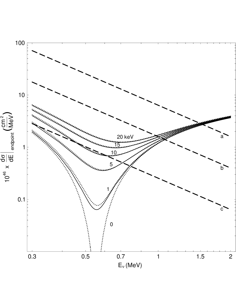
In this paper we show that the inclusion of radiative corrections affects the presence of the dynamical zeros only very mildly, and have therefore no appreciable impact on the applicability of the dynamical zeros. Moreover, we demonstrate that the effect of the finite energy resolution leads to a gradual smearing of the sharp “dip” which appears in the cross section in the vicinity of the zero when perfect resolution is assumed. Despite this smearing, as shown in fig. 1, for realistic values of the energy resolution one still obtains a clear suppression of the standard contribution compared to that with a non-zero neutrino magnetic moment. Finally, we argue that, by selecting the recoil electrons contained in a forward cone centered around the direction of the momentum of the incident neutrino, despite the resulting loss in statistics, one can in fact improve on the existing bounds on the neutrino magnetic moment.
Lowest Order
Consider the elastic scattering (, , or ) in the frame of reference in which the electron is initially at rest. If we neglect terms of order , where indicates any of the Mandelstam variables intervening in the scattering process and is the boson mass, the lowest-order SM prediction for this elastic differential cross section is, neglecting antineutrino masses, [5]
| (1) |
is the Fermi coupling constant, is the electron mass, (upper sign for , lower sign for ), , and is the squared sine of the weak mixing angle. In this elastic process the electron recoil energy ranges from to , where is the incident antineutrino energy. Also, and are the final electron three-momentum and kinetic energy, , and is the cosine of the angle between the momenta of the recoil electron and incident antineutrino. Note that eq. (1) is derived averaging over the polarizations of the initial-state electrons and summing over their final-state helicities. The corresponding formula for neutrino–electron scattering is simply obtained from eq. (1) by interchanging and .
Some time ago the authors of ref. [4] showed the existence of dynamical zeros in the helicity amplitudes for antineutrino–electron elastic scattering at lowest order in the SM. These zeros are not induced by a symmetry of the SM Lagrangian, but by a destructive interference between left- and right-handed electron contributions to the amplitudes. Their location depends on the values of the fundamental parameters and . In particular, for scattering of electron antineutrinos on electrons, the additional charged current contribution to provides the appropriate cancellation with . On the other hand, for scattering of electron neutrinos on electrons, the interference between right and left couplings induced by charged and neutral current amplitudes is constructive. The analysis of ref. [4] furnishes all the information concerning dynamical zeros for both unpolarized and polarized differential cross sections (the analytic formulae for the differential cross sections of the elastic – and – scatterings with all polarization states specified were computed in [6]). For reasons of experimental simplicity we will concentrate here only on the unpolarized case, but refer the reader to [6, 7] for interesting opportunities offered by the study of polarization effects in (anti)neutrino–electron scattering.
The differential cross section in eq. (1) for vanishes exactly for antineutrino energy
| (2) |
and maximum corresponding electron recoil energy (i.e., backward outgoing neutrino and forward electron). We should emphasize that lies inside the range of the reactor antineutrino spectrum (in fact, it is around the peak – see fig. 2), and forward electrons with maximum recoil energy provide a favorable kinematic configuration from the experimental point of view. Note that there are no dynamical zeros in the unpolarized differential cross section of , with only neutral currents. Following ref. [4], the use of this interesting kinematic configuration for the search for physics beyond the SM has been advocated in a number of detailed studies [8, 9, 10].
Figure 1 shows various plots of the differential cross section for the elastic scattering at maximum electron recoil energy as a function of the incident antineutrino energy . The dotted line labeled by “0” is the lowest-order prediction provided by eq. (1). The dynamical zero for is clearly recognizable. Consider now the average of the lowest-order differential cross section in the endpoint region ,
| (3) |
This function of is plotted in fig. 1 for five different values of the energy range 1, 5, 10, 15 and 20 keV (dotted lines). If is the energy interval corresponding to the experimental energy resolution, these lines clearly show how the “dip” corresponding to the dynamical zero gets increasingly filled up by the decrease in energy resolution. The remaining lines in the figure will be discussed in the following sections. Note that the atomic binding of the target electrons has been assumed to be negligible because the dynamical zero occurs at and , a very high value of the electron energy when compared with its binding. However, we refer the reader to ref. [11] for a detailed study of this issue for targets characterized by very high electron binding energies.
Radiative Corrections
As we already pointed out earlier, the dynamical zero of the elastic scattering is not protected by any symmetry of the SM Lagrangian and radiative corrections could significantly modify the lowest-order analysis presented in the previous section. Moreover, the zero occurs at the endpoint of the electron spectrum – an exceptional kinematic configuration, as we will now discuss. To address corrections, a few considerations are in order. As we mentioned earlier, we neglect terms of order . Within this approximation, which is excellent for present experiments, the corrections to this process can be naturally divided into two classes. The first, which we will call “QED” corrections, consists of the photonic radiative corrections that would occur if the theory were a local four–fermion Fermi theory rather than a gauge theory mediated by vector bosons; the second, which we will refer to as the “electroweak” (EW) corrections, will be the remainder. The split-up of the QED corrections is sensible as they form a finite (both infrared and ultraviolet) and gauge-independent subset of diagrams. We refer the reader to ref. [12] for a detailed study of this separation. The QED corrections were first studied in the 1960s in the pioneering articles of Lee and Sirlin [13], and Ram [14] in the framework of an effective four-fermion V–A theory, and further investigated in several subsequent articles [15, 16]. We will use the complete results for the QED corrections to the final electron spectrum which became available only a few years ago [16]. The EW corrections were computed by many authors [17, 18]; we will employ the compact expressions of ref. [18].
The SM prediction for the differential cross section , where indicates the possible emission of a photon, can be cast, up to corrections of , in the following form:
| (4) | |||||
The functions ( or ) describe the QED effects of real and virtual photons [16], while the deviations of the functions and from the lowest-order values and reflect the effect of the electroweak corrections [18].
As it was noted in refs. [14, 18], the functions contain a term which diverges logarithmically at the end of the spectrum, i.e. for , which is precisely the kinematic configuration required for the vanishing at of the lowest-order differential cross section in eq. (1). This feature, related to the infrared divergence, is similar to the one encountered in the QED corrections to the –decay spectrum [19, 20]. If gets very close to the endpoint we have , clearly indicating a breakdown of the perturbative expansion and the need to consider multiple-photon emission. However, this divergence can be easily removed, in agreement with the KLN theorem [20, 21], by integrating the differential cross section over small energy intervals corresponding to the experimental energy resolution, as we did in eq. (3) for the lowest-order prediction,
| (5) |
We are thus ready to assess the impact of the corrections on the dynamical zero of the lowest-order differential cross section. The solid lines in fig. 1 represent, as a function of , the average of the SM differential cross section in the endpoint region up to corrections of (i.e., eq. (5)). As for the lowest-order dotted lines (see previous section), the label next to each solid line indicates one of the five values of the energy range 1, 5, 10, 15 and 20 keV. There is no solid line labeled “0”, as is not defined at the endpoint . Comparing each dotted line for the lowest-order prediction with the corresponding solid one inclusive of corrections, we conclude that, in all cases considered, the effect of the lowest-order dynamical zero is only mildly influenced by the inclusion of radiative corrections111 This analysis is based on the electron spectrum of eq. (4), which includes the bremsstrahlung radiation (real photons) emitted in the scattering process. In bremsstrahlung events, however, some detectors do not measure the electron energy separately, but only a combination of and the energy of the photon (see [16] for a detailed study of this issue). For this reason, we repeated our analysis using the QED corrections of ref. [16] appropriate for detectors measuring the total combined energy of the recoil electron and the possible accompanying photon. Although different from those appearing in eq. (4), also these corrections have no appreciable influence on the effect of the lowest-order dynamical zero.. This relative stability under radiative corrections of the effect of the dynamical zero provides solid foundations to all previous analyses based on this favorable kinematic configuration.
Neutrino Magnetic Moment
The dynamical zero of the SM differential cross section in eq. (1) provides an excellent opportunity to unveil or constrain “new physics” effects. In particular, refs. [4, 9] advocated the possibility of employing it to search for a neutrino magnetic moment.
If neutrino masses are neglected, a neutrino magnetic moment of magnitude increases the SM differential cross section for the elastic scattering by [22]
| (6) |
The measurement of a recoil differential spectrum larger than expected could thus signal the existence of a neutrino magnetic moment, especially if it is characterized by the distinctive low-energy enhancement. To this end, it is important to minimize the detection threshold for the electron recoil energy – a difficult task, given the generally increasing detector background with decreasing energy. On the other hand, as first pointed out in ref. [4], rather than looking for regions of lowest possible energies where the differential cross section in eq. (6) becomes large enough to be comparable with the SM spectrum of eq. (1), one can take advantage of the dynamical zero of the latter. This can be immediately appreciated by looking at the three dashed lines in fig. 1, which represent at maximum electron recoil energy for three different values of the neutrino magnetic moment: , which is the current experimental 90% CL upper bound by the MUNU collaboration [23], , and . Electron antineutrinos with energy around could therefore provide the possibility to study low values of . This interesting conclusion was reached in ref. [4] studying the lowest-order SM cross section and, as we showed in the previous section, the analysis of that reference is only mildly modified by the inclusion of radiative corrections. For this reason, in the remaining part of this article we will simplify our analysis by employing the lowest-order SM cross section given by eq. (1), instead of the one inclusive of corrections, eq. (4).
Antineutrinos of incident energy can be selected from a continuous spectrum source by measuring both energy and direction of the electrons recoiling from the elastic scattering. This can be realized with detectors like the one of MUNU, an experiment carried out at the Bugey nuclear power reactor, designed to study elastic scattering at low energy [23, 24]. The differential cross section measured at reactor antineutrino experiments can be compared with the theoretical prediction given in terms of
| (7) |
where the subscript “TH” stands for “0” or “M” and is the normalized antineutrino spectrum incident at the detector. is the minimum required to produce an electron with recoil energy . If the recoil angle can also be measured, then the analysis can be restricted to events with electrons recoiling in the forward cone (note that for a given value of , the recoil electrons are restricted by kinematics to lie in the cone ). Instead of eq. (7), the theoretical prediction to match this selective measurement is
| (8) |
where the upper limit of integration is now and . Clearly, is the limit of for . For a given value of , we can thus select incident antineutrinos with energies by rejecting events with . In particular, incident antineutrinos with can be selected by considering only electrons in a small forward cone .
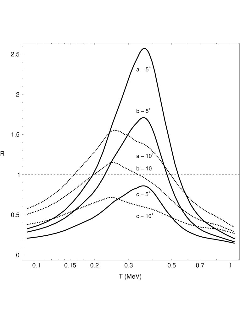
To study the sensitivity of the theoretical prediction to the neutrino magnetic moment when the recoil electrons are contained in the forward cone , we introduce the ratio
| (9) |
This ratio is plotted in fig. 3 as a function of for three different values of . Solid lines indicate the ratio for , while dotted lines, labeled by “no cuts”, represent the same ratio obtained without restricting the angle of the recoiling electrons (i.e., ). The normalized reactor antineutrino spectrum of ref. [25] has been used for , see fig. 2. For , fig. 3 shows that the value of for which the convoluted magnetic moment cross section becomes equal to the SM one moves from to if the recoil electrons are contained in a forward cone. The same angular restriction shifts from to the value of for which the magnetic moment cross section for equals 50% of the SM one. Also from fig. 3 it can be seen that while at 250 keV for is only about 5% of , by discarding events with the two cross sections become almost equally large. The upshot is that angular cuts on the final-state electrons move the sensitivity to higher (and thus more accessible) electron energies. We should point out that once the electron energy is fixed, the larger the value of , the smaller the upper bound in the definition of eq. (8). This implies that increasing the value of also increases the relative systematic uncertainty of the convoluted cross section due to the lack of precise knowledge of the low energy part of the reactor antineutrino spectrum. On the other hand, the great advantage of going to regions where is large is that the sensitivity to this systematic uncertainty is dramatically diminished [26].
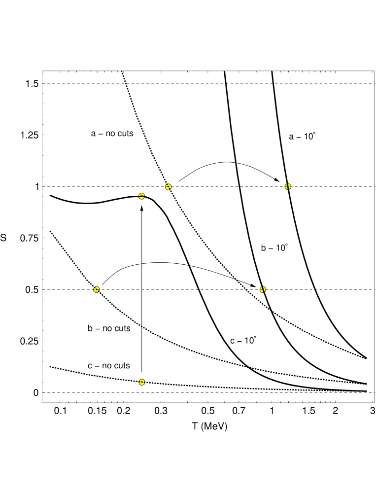
This remarkable opportunity to overcome serious experimental limitations in the search for neutrino magnetic moments, such as high backgrounds at low energies, must certainly be confronted with the loss in statistics induced by the angular selection. As the sensitivity to in direct search experiments scales as , where is the number of signal events, we introduce the function defined by
| (10) |
The square root expression multiplying takes into account the loss of statistical accuracy caused by the rejection of events with . A figure of merit is provided in fig. 4, where the ratio (as an example, the value employed by the MUNU Collaboration has been chosen as reference) is plotted for and . Figure 4 indicates that high values of the sensitivity , due to the selection of electrons contained in a narrow forward cone, can overcompensate the loss in statistics induced by this angular selection, provided the cone can be narrowed sufficiently. Therefore, apart from the previously discussed opportunities to reduce systematic uncertainties, the search for can actually benefit from an angular restriction even from the purely statistical analysis illustrated in fig. 4. Indeed, fig. 4 shows that for and (the current upper bound), is larger than one for in the range . Higher ratios are obtained for , in a slightly higher energy range. Following the conclusions of our previous paragraph on the benefits of the angular selection in overcoming systematic limitations, we will finally note that even analyses with , although statistically disfavoured, might still provide a better opportunity to search for than employing a large cone. Dedicated experimental studies, with realistic backgrounds and systematic uncertainties, should address this delicate issue and make an analysis with real data.
Conclusions
It is known that, due to a destructive interference between charged and neutral current amplitudes, a dynamical zero appears in the lowest-order SM cross section describing the elastic scattering. In this article we studied several main issues related to the applicability of this dynamical zero as a method for improving the bounds on the values of the neutrino magnetic moment. In particular, by means of a detailed analysis we demonstrated that the lowest-order dynamical zero remains essentially unaffected by the inclusion of the radiative corrections and, for realistic values of , finite energy resolution still allows for the isolation of possible “new physics” contributions related to the presence of a non-standard neutrino magnetic moment.
Having established the persistence of the dynamical zero effects under radiative corrections, we proceeded to argue that the experimental isolation of events near the region of this special configuration is in fact advantageous, despite the obvious loss in statistics. The overcompensating factor originates from the fact that, when the corresponding angular cuts are imposed on the final-state electrons, the sensitivity to increases and moves to higher, and therefore more accessible, electron energies. A high sensitivity to also diminishes the sensitivity to systematic uncertainties. In addition, for discussed values of , the signal function , defined in eq. (10) to take into account the loss in statistics, is larger, in a specific range of the recoil electron energy, for a small angular cone rather than for a large one. Our results suggest that an analysis with real data is worth to be done.
Acknowledgments
It is a pleasure to thank C. Broggini and P. Minkowski for very useful discussions. This work was supported by the MECyD fellowship SB2002-0105, the MCyT grant FPA2002-00612, and by the European Union under contract HPRN-CT-2000-00149.

References
- [1] B.W. Lee and R.E. Shrock, Phys. Rev. D 16 (1977) 1444.
- [2] S. Eidelman et al. [Particle Data Group Collaboration], Phys. Lett. B 592 (2004) 1.
- [3] K.S. Babu and R.N. Mohapatra, Phys. Rev. Lett. 63 (1989) 228; R. Barbieri, M.M. Guzzo, A. Masiero and D. Tommasini, Phys. Lett. B 252 (1990) 251; S.M. Barr, E.M. Freire and A. Zee, Phys. Rev. Lett. 65 (1990) 2626.
- [4] J. Segura, J. Bernabeu, F.J. Botella and J. Penarrocha, Phys. Rev. D 49 (1994) 1633 [arXiv:hep-ph/9307278].
- [5] G. ’t Hooft, Phys. Lett. B 37 (1971) 195.
- [6] P. Minkowski and M. Passera, Phys. Lett. B 541, 151 (2002) [arXiv:hep-ph/0201239]; Nucl. Phys. Proc. Suppl. 118, 495 (2003).
- [7] T.I. Rashba and V.B. Semikoz, Phys. Lett. B 479 (2000) 218; S. Ciechanowicz, W. Sobkow and M. Misiaszek, arXiv:hep-ph/0309286.
- [8] J. Segura, J. Bernabeu, F.J. Botella and J.A. Penarrocha, Phys. Lett. B 335, 93 (1994) [arXiv:hep-ph/9406305].
- [9] J. Segura, Eur. Phys. J. C 5, 269 (1998) [arXiv:hep-ph/9708298]; O.G. Miranda, J. Segura, V.B. Semikoz and J.W.F. Valle, arXiv:hep-ph/9906328.
- [10] J. Bernabeu and S. Palomares-Ruiz, JHEP 0402, 068 (2004) [arXiv:hep-ph/0311354].
- [11] S.A. Fayans, L.A. Mikaelyan and V.V. Sinev, Phys. Atom. Nucl. 64 (2001) 1475 [Yad. Fiz. 64 (2001) 1551].
- [12] A. Sirlin, Rev. Mod. Phys. 50 (1978) 573; Phys. Rev. D22 (1980) 971.
- [13] T.D. Lee and A. Sirlin, Rev. Mod. Phys. 36 (1964) 666.
- [14] M. Ram, Phys. Rev. 155 (1967) 1539.
- [15] E.D. Zhizhin, R.V. Konoplich, Y.P. Nikitin, and B.U. Rodionov, JETP Lett. 19 (1974) 36; E.D. Zhizhin, R.V. Konoplich and Y.P. Nikitin, Sov. Phys. J. 18 (1975) 1709, translated from Izv. Vuz, Fiz. 12 (1975) 82; Elementary particles and cosmic rays, Atomizdat, Moscow, 1976, 57–71 (in Russian); K. Aoki and Z. Hioki, Prog. Theor. Phys. 66 (1981) 2234; Z. Hioki, Prog. Theor. Phys. 67 (1982) 1165; D.Y. Bardin and V.A. Dokuchaeva, Sov. J. Nucl. Phys. 39 (1984) 563; Nucl. Phys. B246 (1984) 221; Sov. J. Nucl. Phys. 43 (1986) 975; J. Bernabeu, S.M. Bilenky, F.J. Botella and J. Segura, Nucl. Phys. B426 (1994) 434; C. Broggini, I. Masina and M. Moretti, Phys. Lett. B 452 (1999) 137.
- [16] M. Passera, Phys. Rev. D 64 (2001) 113002 [arXiv:hep-ph/0011190]; J. Phys. G 29 (2003) 141 [arXiv:hep-ph/0102212].
- [17] P. Salomonson and Y. Ueda, Phys. Rev. D11 (1975) 2606; M. Green and M. Veltman, Nucl. Phys. B169 (1980) 137; Erratum–ibid. B175 (1980) 547; W.J. Marciano and A. Sirlin, Phys. Rev. D22 (1980) 2695; K. Aoki, Z. Hioki, R. Kawabe, M. Konuma and T. Muta, Prog. Theor. Phys. 65 (1981) 1001; S. Sarantakos, A. Sirlin and W.J. Marciano, Nucl. Phys. B217 (1983) 84.
- [18] J.N. Bahcall, M. Kamionkowski and A. Sirlin, Phys. Rev. D51 (1995) 6146.
- [19] R.E. Behrends, R.J. Finkelstein and A. Sirlin, Phys. Rev. 101 (1956) 866.
- [20] T. Kinoshita and A. Sirlin, Phys. Rev. 113 (1959) 1652.
- [21] T. Kinoshita, J. Math. Phys. 3 (1962) 650; T.D. Lee and M. Nauenberg, Phys. Rev. 133 (1964) B1549.
- [22] A.V. Kyuldjiev, Nucl. Phys. B 243 (1984) 387.
- [23] Z. Daraktchieva et al. [MUNU Collaboration], Phys. Lett. B 564 (2003) 190 [arXiv:hep-ex/0304011].
- [24] C. Amsler et al. [MUNU Collaboration], Nucl. Instrum. Meth. A 396 (1997) 115; M. Avenier et al. [MUNU Collaboration], Nucl. Instrum. Meth. A 482 (2002) 408 [arXiv:hep-ex/0106104].
- [25] V.I. Kopeikin, L.A. Mikaelyan and V.V. Sinev, Phys. Atom. Nucl. 60 (1997) 172 [Yad. Fiz. 60 (1997) 230].
- [26] H.B. Li and H.T. Wong, J. Phys. G 28, 1453 (2002) [arXiv:hep-ex/0111002].