Master integrals for massive two-loop Bhabha scattering in QED

Abstract

We present a set of scalar master integrals (MIs) needed for a complete treatment of massive two-loop corrections to Bhabha scattering in QED, including integrals with arbitrary fermionic loops. The status of analytical solutions for the MIs is reviewed and examples of some methods to solve MIs analytically are worked out in more detail. Analytical results for the pole terms in $\epsilon$ of so far unknown box MIs with five internal lines are given.

I Introduction

Bhabha scattering is proposed to be measured at the International Linear Collider (ILC) in the very forward direction with a precision that would allow to determine the luminosity with an accuracy of 10^-4 Aguilar-Saavedra:2001rg ; Hawkings:1999ac ; Lohmann:2004nn ; Lohmann:2004nn2 . The Monte Carlo programs which were in use for the analysis of LEP data aimed at a slightly lower accuracy, and one could neglect certain two-loop corrections there; for a discussion see Jadach:2003zr . At the ILC, the theoretical prediction of the differential cross section for Bhabha scattering

$$e^{+}(p_{2})+e^{-}(p_{1})\to e^{+}(p_{4})+e^{-}(p_{3})$$ (1)

has to include the complete virtual photonic two-loop corrections. This is a highly nontrivial task, but with substantial recent progress in several directions. Here, we will concentrate mainly on efforts to determine the two-loop corrections in a calculational scheme with a finite electron mass $m$, and with a regularization of both UV and IR divergences with dimensional regularization . Because the Monte Carlo programs for the treatment of real bremsstrahlung assume a finite photon mass at intermediate states of the calculation Jadach:1996is ; Melles:1997qa ; Arbuzov:1995qd ; Arbuzov:1996jj , one will have to care about this fact when results will be finally combined. This might be done similarly as in Glover:2001ev ; Mastrolia:2003yz . Alternatively, the soft photon bremsstrahlung can be recalculated completely in $D$ dimensions as in Bonciani:2004qt , where this is done for the simplest subset of the corrections.

In the QED model with three leptonic flavors one has 154 Feynman diagrams (with all the 1PI diagrams, but without loops in external lines), among them 68 double-box diagrams web-masters:2004nn . Besides the usual problems of efficient bookkeeping, the main problem is the evaluation of the loop integrals. One has to solve Feynman integrals with $L\leq 2$ loops and $N\leq 7$ internal lines,

$$G(X) = \frac{1}{\left(i\pi^{d/2}\right)^{L}}\int\frac{d^{D}k_{1}\ldots d^{D}k_{L}~{}~{}X}{(q_{1}^{2}-m_{1}^{2})^{\nu_{1}}\ldots(q_{j}^{2}-m_{j}^{2})^{\nu_{j}}\ldots(q_{N}^{2}-m_{N}^{2})^{\nu_{N}}},$$ (2)

where $X=1,k_{1\alpha},k_{1\alpha}k_{2\beta},\ldots$ stands for tensors in the loop momenta. This might be done by a procedure with three subsequent steps:

• reduce all tensorial loop integrals to scalar integrals,

• reduce these to a smaller set of scalar master integrals (MIs),

• evaluate the MIs.

A completely numerical approach might also be possible Passarino:2004nn . For checks in the Euclidean region this has been proven to be a powerful tool Binoth:2000ps ; Binoth:2003ak ; see Appendix A.

Step (i) may be considered to be solved by now, the second one is solved for Bhabha scattering with this article , and step (iii) is solved for all self energies and vertices, but remains largely unsolved for the two-loop boxes. So, the evaluation of the two-loop boxes is the remaining bottleneck. Indeed, very few of the 33 double-box master integrals have been determined completely Smirnov:2001cm ; Bonciani:2003cj ; Heinrich:2004iq ; Czakon:2004tg or to some extent Heinrich:2004iq .

The article is organized as follows. In Section II, the diagrams and prototypes for two-loop Bhabha scattering are identified and the method for their evaluation in terms of MIs is outlined. We discuss in Section III the complete set of MIs and give an overview with figures and tables. The status of analytical (or semi-analytical) solutions of the known MIs is summarized. Some typical techniques for MI evaluation are demonstrated. The section includes also a discussion of MIs with numerators. We close with a Summary. Appendix A includes an extension of the numerical method for the evaluation of Feynman diagrams with sequential sector decompositions, which allows to treat integrals with irreducible numerators. The final Appendix B defines a complete and compact set of Harmonic Polylogarithms up to weight 4.

II From diagrams to prototypes and master integrals

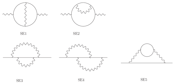
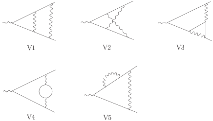
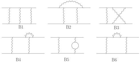
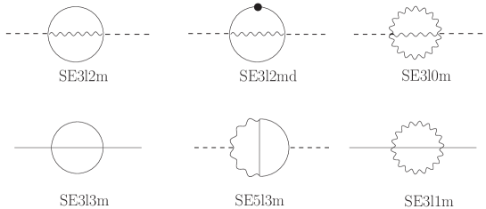
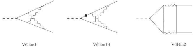
In a theory with only electrons and photons, one has in the ’t Hooft-Feynman gauge 52 1PI two-loop Feynman diagrams, all of the double-box type. After adding to this number the 1P-reducible diagrams without loop insertions in external lines, there are 94 diagrams. We will call this the one-flavor case . Due to the existence of up to two closed fermion loops in certain diagrams, a complete picture of the process arises when besides the electron two additional flavors are taken into account. Then, there are 68 double boxes and 154 two-loop Feynman diagrams in total . Fortunately, there are much less two-loop structures to be calculated; they are represented by prototypes. Prototypes are irreducible (sub)diagrams of a certain topology with account of the various, different masses of internal lines. All the Feynman integrals $G(X)$ (see (2)) with the same topology and propagators, but with arbitrary powers $\nu_{i}>0$ of these propagators, and potentially with irreducible numerators $X$ correspond to one prototype. In Figures 1 to 3 we show the sets of two-loop self-energy, vertex and box diagrams for which the scalar MIs are needed. As mentioned, there are two bosonic self energies SE1 and SE2, and the other three fermionic self energies renormalize the external lines. Further, there are five two-loop vertex and six two-loop box diagrams for Bhabha scattering.

Technically, one has to calculate all the Feynman integrals $G(X)$ related to these diagrams by a reduction of integrals with irreducible numerators $X$ and denominators with higher powers $\nu_{i}$ to a smaller set of scalar master integrals.

Figure 1: The two-loop self-energy diagrams for massive Bhabha scattering. SE3 to SE5 are needed for the renormalization of external fermion lines.

Figure 2: The two-loop vertex diagrams for massive Bhabha scattering.

Figure 3: The two-loop box diagrams for massive Bhabha scattering.

We have determined such a set of scalar MIs for the virtual two-loop corrections to Bhabha scattering with the Laporta-Remiddi algorithm Laporta:1996mq ; Laporta:2001dd . Realizations of the algorithm are SOLVE Remiddi:2004nn , the Maple program AIR Anastasiou:2004vj , and the C++ library DiaGen/IdSolver Czakon:2004uu2 . We use DiaGen/IdSolver , which allows to tackle two problems: (i) derive an appropriate set of algebraic equations with integration by parts (IBP) Chetyrkin:1981qh and Lorentz invariance (LI) identities Gehrmann:1999as , and (ii) determine a list of master integrals by solving this set of equations. The procedure is heuristic. To be safe about the completeness of the solution, one has to solve the system of equations to high powers of numerators and denominators. If the coefficients are kept as exact functions of the kinematical variables $s,t,m^{2}$ (and for several flavors of a further scale $M^{2}$), the algorithm is time and computer memory consuming. To minimize computer ressources usage, evaluation homomorphisms are used, i.e. the system is solved by projecting the coefficients to the field of rational numbers with suitably chosen values of the parameters. Let us mention that, from the point of view of complexity, the complete two-loop Bhabha scattering calculation with massless fermions is as complicated as the two-loop massive vertex case: on a 2 GHz Pentium PC with 1 GB memory, it takes minutes to be solved. Further, the number of MIs is moderate, e.g. 5 massless MIs compared to 22 MIs for the massive box diagram B3.

There is some arbitrariness in the choice of masters. We prefer to present a set of MI without numerators. But we then have to allow for higher powers of propagators ($\nu_{i}>1$, dotted lines). This choice has one basic advantage: the MIs are independent of the momenta flowing inside loops. Of course, in the set of solutions for MIs, there are algebraic relations between scalar integrals with numerators and those with dotted denominators: so one always has a freedom of choice. For an explicit evaluation of the MIs, this is of importance; see the discussions in the subsequent sections.

In Table 1 we give a list of the net numbers of (two-loop)+(one-loop) master integrals needed for the evaluation of all two-loop vertex and box diagrams for the one-flavor case. The case of several flavors is separately discussed in Section III.6.

III Master Integrals

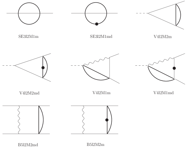
Here we will describe the sets of master integrals needed for the calculation of all Feynman integrals for the diagrams in Figures 1 to 3. We use a nomenclature where e.g. V3l2m is the name of the integral for a Vertex with 3 lines, among them 2 massive lines; B5l4md is the name of the integral for a Box with 5 lines, among them 4 massive lines and one line with a dot. Sometimes there are several candidates for the same name, e.g. V6l4m1 and V6l4m2 in Figure 6, or V4l1m1d1 and V4l1m1d2 in Figure 8.

Because they are lengthy, we give in this article practically no explicit expressions for the master integrals. Instead, for all the self energies and vertices, they may be found in web-masters:2004nn in form of a human readable Mathematica file, MastersBhabha.m. We determined all these MIs, and several of the box masters, in terms of Harmonic Polylogarithms (HPLs) Remiddi:1999ew . The file allows a determination of the expressions in form of polylogarithms. We used HPLs up to the weight 4 and give in Appendix B a complete basis for their systematic calculation. The complete list of HPLs may be found in the Mathematica file HPL4.m in web-masters:2004nn . Numerical checks were performed with the numerical integration package sectors.m, see Appendix A.

We evaluated most of the MIs with the method of differential equations Kotikov:1991hm ; Remiddi:1997ny , which has been described in detail in many papers, e.g. Laporta:2001dd ; Bonciani:2003cj ; Bonciani:2003hc ; Bonciani:2003te , and we will not repeat this here. Nevertheless, it might be useful to indicate some technical details of our calculations. The master integrals are defined in a Minkowskian metric, and the external momenta are introduced in (1). With $(p_{1}+p_{2})=(p_{3}+p_{4})$ and $p_{i}^{2}=m^{2}$, we define $s=(p_{1}+p_{2})^{2},\;t=(p_{1}-p_{3})^{2},\;u=(p_{1}-p_{4})^{2}$. The analytical results are expressed by dimensionless variables $x$ and $y$,

$$x=\frac{\sqrt{-s+4}-\sqrt{-s}}{\sqrt{-s+4}+\sqrt{-s}},$$ (3)

corresponding to $s=-(1-x)^{2}/x$, and $y$ is obtained by replacing $s$ by $t$. We set the electron mass to unity, $m^{2}=1$.

In the rest of the article, we discuss the set of master integrals and their expansions in the parameter $\epsilon=(4-D)/2$. First we treat only electrons and photons. The diagrams with additional flavors and thus with a second mass scale are discussed in Section III.6.

III.1 One-loop Master Integrals

There are five one-loop master integrals needed for the evaluation of the two-loop diagrams; see Figure 4. Our normalization of the momentum integrals is chosen such that the one-loop tadpole becomes:

$${\tt T1l1m} = \frac{e^{\epsilon\gamma_{E}}}{i\pi^{D/2}}\int\frac{d^{D}q}{q^{2}-1}=\frac{1}{\epsilon}+1+\left(1+\frac{\zeta_{2}}{2}\right)\epsilon+\left(1+\frac{\zeta_{2}}{2}-\frac{\zeta_{3}}{3}\right)\epsilon^{2}+\ldots$$ (4)

For completeness, we should mention that a full calculation of the Bhabha scattering process (1) also includes the one loop corrections in the electroweak Standard Model (plus some higher order corrections). For their treatment we refer to Consoli:1979xw ; Bohm:1984yt ; Bohm:1986fg ; Bardin:1990xe ; Bardin:1997xq ; Beenakker:1997fi ; Bardin:1999yd ; Kobel:2000aw ; Gluza:2004tq ; Lorca:2004dk ; Lorca:2004fg .

Figure 4: The five one-loop MIs. External solid (dashed) lines describe on- (off-)shell momenta.

III.2 Two-loop 2-point Master Integrals

There are six two-loop 2-point MIs; see Figure 5. The MI SE3l0m may be expressed by two subsequent one-loop momentum integrations in terms of $\Gamma$ functions whose $\epsilon$-expansion is trivial 'tHooft:1972fi ; Surguladze:1989ez . Explicit expressions may also be found in Bonciani:2003hc , quoted from Bonciani:2001 . The MIs SE3l1m and SE3l3m for the renormalization of external fermion legs are needed only on the mass shell; they may be calculated with ON-SHELL2 Fleischer:1999tu , with an appropriate change of normalization with respect to (4). For MI SE3l3m see also Broadhurst:1990ei ; Broadhurst:1991fi . The MI SE5l3m was first calculated to ${\cal O}(1)$ in Broadhurst:1990ei (see also Fleischer:1998nb ) and to ${\cal O}(\epsilon)$ in Davydychev:2003mv ; Bonciani:2003hc . The two remaining MIs SE3l2m = SE3l2m(1,1,1,0) and SE3l2md = SE3l2m(1,1,2,0) are defined by:

$${\tt SE3l2m}(a,b,c,d) = =-\frac{e^{2\epsilon\gamma_{E}}}{\pi^{D}}\int\frac{d^{D}k_{1}d^{D}k_{2}~{}~{}(k_{1}k_{2})^{-d}}{[(k_{1}+k_{2}-p)^{2}-m^{2}]^{b}~{}[k_{1}^{2}]^{a}~{}[k_{2}^{2}-m^{2}]^{c}}.$$ (5)

These two MIs have been expressed in Fleischer:1999hp in terms of T1l1m and the functions SE3l2m(1,2,2,0) and SE3l2m(1,1,3,0), and the $\epsilon$-expansion is determined there (after equation (15)) in terms of polylogarithms.

An equivalent result, in terms of HPLs, is given in Bonciani:2003te , where the integrals SE3l2m and SE3l2mN = SE3l2m(1,1,1,–1) have been chosen as masters. By an algebraic relation, valid for $m^{2}=1$ and $p^{2}=s$,

$${\tt SE3l2md} = \frac{-(1+s)+\epsilon(2+s)}{s-4}~{}{\tt SE3l2m}+\frac{2(1-\epsilon)}{s-4}\left({\tt T1l1m}^{2}+3~{}{\tt SE3l2mN}\right),$$ (6)

one may derive then SE3l2md.

For a direct determination of the MIs with differential equations, we constructed a differential operator for the self energies using the scaling property:

$${\tt SE}(\lambda p^{2},\lambda m^{2})=\lambda^{\text{dim}[{\tt SE}(p^{2},m^{2})]}~{}{\tt SE}(p^{2},m^{2}),$$ (7)

where $\text{dim}({\tt SE})$ is the dimension of the 2-point MI ${\tt SE}$. The differential operator is:

$$s\frac{\partial}{\partial s}{\tt SE}(s,m^{2})=-m^{2}\frac{\partial}{\partial m^{2}}{\tt SE}(s,m^{2})+\text{dim}[{\tt SE}(s,m^{2})]~{}{\tt SE}(s,m^{2}).$$ (8)

With this operator, one may derive coupled differential equations for the two masters and solve them with account of boundary conditions at the kinematical point $s=0$. Because the integral SE3l2md is one of our masters, we reproduce it here explicitely:

$${\tt SE3l2md}(x) = \frac{1}{2\epsilon^{2}}+\frac{1}{2\epsilon}-\left(\frac{1-\zeta_{2}}{2}+\frac{1+x}{1-x}H[0,x]+\frac{1+x^{2}}{(1-x)^{2}}H[0,0,x]\right)+{\cal O}(\epsilon).$$ (9)

In Tables 2 and 3, we list for each of the diagrams the MIs needed for their evaluation. Masters denoted by an asterisk are of one-loop type.

Figure 5: The six two-loop 2-point MIs. External solid (dashed) lines describe on (off) -shell momenta.

III.3 Two-loop 3-point Master Integrals

There are nineteen two-loop 3-point MIs for Bhabha scattering. They are shown in Figures 6 to 8. The equations for vertex MIs may be obtained with a differential operator:

$$s\frac{\partial}{\partial s}=\frac{1}{4-s}\left[2p_{2}^{\mu}\frac{\partial}{\partial p_{1}^{\mu}}+(2-s)p_{1}^{\mu}\frac{\partial}{\partial p_{1}^{\mu}}\right].$$ (10)

Another operator can be obtained by the exchange $p_{1}\leftrightarrow p_{2}$.

In Table 3 we list all the vertex MIs for the various diagrams of Figure 2. The MIs for the evaluation of the QED (and QCD) vertex diagrams are worked out in Bonciani:2003te ; Bonciani:2003hc . The four MIs of prototypes V5l2m1 and V5l2m2 are additionally needed for the evaluation of box diagrams B1 to B4 and have been determined in Czakon:2004tg . It was possible to determine all the vertex MIs with the method of differential equations. When dotted masters (or those with irreducible numerators) are involved one has to treat a system of coupled first order linear equations. For prototype V4l1m1, three masters had to be treated together.

Figure 6: The three two-loop vertex MIs with six internal lines.

Figure 7: The six two-loop vertex MIs with five internal lines.

Figure 8: The ten two-loop vertex MIs with four internal lines.

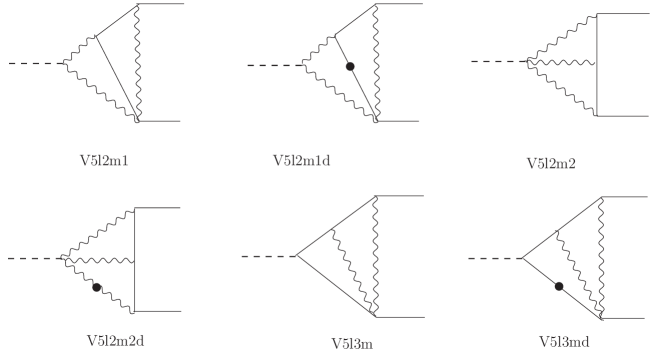
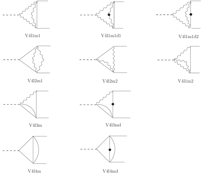
As an instructive example for the use of coupled differential equations we will study here the prototype V5l2m2. For few selected examples, we applied also alternative methods of calculation in order to have some cross checks; see also Czakon:2004wu . Two of them will also be exemplified here. One method (for MI V4l1m2) implies the integration over an UV divergent subloop and a subsequent subtraction in order to isolate an additional UV singularity, and the other one (for MI V5l2m2) introduces a subtracted dispersion relation.

III.3.1 The master integrals for the prototype V5l2m2

The prototype

$${\tt V5l2m2}(a,b,c,d,e;h,i) = -\frac{e^{2\epsilon\gamma_{E}}}{\pi^{D}}\int\frac{d^{D}k_{1}d^{D}k_{2}~{}(p_{1}k_{2})^{-h}~{}(p_{2}k_{2})^{-i}}{[(k_{1}+k_{2})^{2}-m^{2}]^{a}[k_{2}^{2}-m^{2}]^{b}[(p_{1}-k_{1}-k_{2})^{2}]^{c}[k_{1}^{2}]^{d}[(k_{2}-p_{3})^{2}]^{e}}$$ (11)

has the masters V5l2m2 = V5l2m2(1,1,1,1,1;0,0) and V5l2m2d = V5l2m2(1,1,1,1,2;0,0), together with simpler ones. They contribute to the box diagrams B1 (planar double box) and B3 (nonplanar double box), see Table 3. The momenta are, with the conventions used here, in the $t$ channel. Applying the corresponding differential operator (42), in the $t$ channel, we wrote the differential equations for the MI V5l2m2 and for V5l2m2N = V5l2m2(1,1,1,1,1;–1,0). One gets:

$$t\frac{\partial}{\partial t}{\tt V5l2m2} = \frac{(-4+s+2t)}{2(-4+s+t)}\Bigl{(}{\tt V4l1m2}[1,1,1,2;0]-{\tt V5l2m2}+2~{}{\tt V5l2m2d}\Bigr{)}$$ (12)

$$-~{}\frac{t}{(-4+s+t)}~{}{\tt V5l2m2}[1,1,1,1,2;0,-1]-~{}{\tt V5l2m2}[1,1,1,1,2;-1,0],$$

$$t\frac{\partial}{\partial t}{\tt V5l2m2N} = \frac{(-4+s+2t)}{4(-4+s+t)}\Bigl{(}2~{}{\tt V4l1m2}[1,1,1,2;-1]-(-2+t)~{}{\tt V4l1m2}[1,1,1,2;0]$$ (13)

$$+~{}4~{}{\tt V5l2m2N}\Bigr{)}+\frac{t}{(-4+s+t)}~{}{\tt V5l2m2}[1,1,1,1,2;-1,-1]-{\tt V5l2m2}[1,1,1,1,2;-2,0].$$

Additional functions at the right hand side are of prototype V4l1m2:

$${\tt V4l1m2}(a,b,c,d;g) = -\frac{e^{2\epsilon\gamma_{E}}}{\pi^{D}}\int\frac{d^{D}k_{1}d^{D}k_{2}~{}(p_{1}k_{2})^{-g}}{[(p_{3}+k_{1}+k_{2})^{2}-m^{2}]^{a}[p_{1}-p_{3}-k_{1}-k_{2}]^{b}[k_{1}^{2}]^{c}[k_{2}^{2}]^{d}}.$$ (14)

Again, we write the basic master V4l1m2 (no dots, no numerators) without arguments.

Besides MIs, at the right hand side of (12) and (13) one meets additional scalar integrals, which have to be expressed by algebraic equations through MIs:

$${\tt V4l1m2}[1,1,1,2;0] = \frac{(1-5\epsilon+6\epsilon^{2})}{2\epsilon t}\left(4~{}{\tt V4l1m2}+\frac{2-3\epsilon}{-1+4\epsilon}{\tt SE3l1m}\right),$$ (15)

$${\tt V4l1m2}[1,1,1,2;-1] = \frac{2-3\epsilon}{4t}\left(-2~{}{\tt SE3l0m}+t~{}{\tt SE3l1m}\right)+\frac{-1+3\epsilon}{2}~{}{\tt V4l1m2},$$ (16)

$${\tt V5l2m2}[1,1,1,1,2;-2,0] = -\frac{(-1+\epsilon)^{2}(-2+4\epsilon(1+\epsilon)+t(1-3\epsilon))}{8(1-2\epsilon)^{2}\epsilon}{\tt T1l1m}^{2}+\frac{\epsilon(1+2\epsilon-t)}{-1+2\epsilon}{\tt V5l2m2}$$ (17)

$$+~{}[(8-2t-t^{2})+\epsilon(-56+18t+6t^{2})+\epsilon^{2}(128-54t-11t^{2})+\epsilon^{3}(-96+60t+2t^{2})]$$

$$\times~{}\frac{(-2+3\epsilon)}{16(-1+2\epsilon)(-1+4\epsilon)}{\tt SE3l1m}-\frac{(-2\epsilon+4\epsilon^{2}-t)(-2+t)}{4\epsilon(-1+2\epsilon)}{\tt V5l2m2d}$$

$$+\frac{(-2+3\epsilon)(-2+\epsilon(8-4t)+\epsilon^{2}(-4+t)+t)}{8\epsilon t}{\tt SE3l0m}$$

$$+~{}\frac{8-6t+t^{2}-2\epsilon(-4+t)(-5+2t)+\epsilon^{2}(48+-20t+t^{2})}{8t}{\tt V4l1m2}$$

Three further expressions may be left out here web-masters:2004nn , but we have to give that for V5l2m2N:

$${\tt V5l2m2N} = \frac{4}{1-2\epsilon}\left(\epsilon~{}{\tt V5l2m2}\right)+\frac{t(1+2\epsilon)}{2\epsilon(-1+2\epsilon)}{\tt V5l2m2d}$$ (18)

$$-\frac{(-2+3\epsilon)(3-17\epsilon+26\epsilon^{2})}{8\epsilon(-1+2\epsilon)(-1+4\epsilon)}{\tt SE3l1m}+\frac{(-1+\epsilon)^{2}(-1+4\epsilon)}{4(1-2\epsilon)^{2}\epsilon}{\tt T1l1m}^{2}$$

$$-\frac{2+9(-1+\epsilon)\epsilon}{4\epsilon^{2}t}{\tt SE3l0m}+\frac{-1+\epsilon}{4\epsilon}{\tt V4l1m2}.$$

This equation may be inverted in order to eliminate V5l2m2d at the right hand side of (12) and (13) in favor of V5l2m2N, V5l2m2, and simpler MIs:

$$t\frac{\partial}{\partial t}{\tt V5l2m2N} = -2\left(\epsilon~{}{\tt V5l2m2}\right)-\frac{(-1+\epsilon)^{2}}{2(-1+2\epsilon)}{\tt T1l1m}^{2}+\frac{2-7\epsilon+6\epsilon^{2}}{2(-1+2\epsilon)(-4+t)}\left({\tt SE3l1m}-{\tt SE3l0m}\right)$$ (19)

$$-~{}\frac{(6-16\epsilon-2t+5\epsilon t)}{2(-4+t)}{\tt V4l1m2},$$

$$t\frac{\partial}{\partial t}{\tt V5l2m2} = \frac{2(1+2\epsilon)-t}{-4+t}{\tt V5l2m2}+\frac{-1+2\epsilon}{-4+t}\left(2~{}{\tt V5l2m2N}+{\tt V4l1m2}\right)$$ (20)

$$+~{}\frac{2-7\epsilon+6\epsilon^{2}}{2(-1+2\epsilon)(-4+t)}{\tt SE3l1m}-\frac{(-1+\epsilon)^{2}}{(-1+2\epsilon)(-4+t)}{\tt T1l1m}^{2}.$$

The dependence on the unknowns in these two equations is such that they decouple as power series in $\epsilon$, and their solution is simplified thereby. Applying the inverted (18), the two masters are determined Czakon:2004tg :

$${\tt V5l2m2} = \frac{2x}{(-1+x^{2})}\left(8\zeta_{4}+2\zeta_{2}H[0,0,x]-4\zeta_{2}H[0,1,x]+H[0,0,0,0,x]+2H[0,0,0,1,x]\right)+\cal{O}(\epsilon),$$ (21)

$${\tt V5l2m2d} = -\frac{x}{4\epsilon^{2}(1-x)^{2}}+\frac{x(1-H[0,x]-2H[1,x])}{2\epsilon(1-x)^{2}}$$ (22)

$$+~{}\frac{x}{4(1-x)^{2}(1+x)}\bigl{[}-4-15\zeta_{2}-4x+\zeta_{2}x+4(1+x)\left(H[0,x]+2H[1,x]\right)$$

$$-~{}2(x+3)\left(H[0,0,x]+2H[0,1,x]\right)-8(1+x)\left(H[1,0,x]+2H[1,1,x]\right)\bigr{]}+\cal{O}(\epsilon).$$

Another interesting opportunity appears when a system has some undotted and dotted masters being both UV finite, but IR divergent, and at the same time a related integral with numerator is both UV and IR finite Czakon:2004wu , as it is the case here. Then, one may determine singularities in $\epsilon$ from the algebraic relations between the functions; here from (18). This way one also gets the divergent parts of (22). This may serve as a cross check here. The dot in V5l2m2d introduces overlapping IR singularities and produces the $1/\epsilon^{2}$ term.

III.3.2 Example: The master integral V4l1m2

The MI V4l1m2 (see Figure 8) has a massless UV divergent subloop:

$${\tt V4l1m2} = -\frac{e^{2\epsilon\gamma_{E}}}{\pi^{D}}\int\frac{d^{D}k_{1}d^{D}k_{2}}{[k_{2}^{2}][(k_{1}+k_{2}-p_{1})^{2}][k_{1}^{2}-1][(k_{1}+p_{2})^{2}]}.$$ (23)

We will use a subtraction procedure in order to isolate the remaining UV singularity. The two momentum integrations may be performed subsequently:

$$\int\frac{d^{D}k_{2}}{[k_{2}^{2}][(k_{2}+k_{1}-p_{1})^{2}]} = i\pi^{D/2}\frac{\Gamma(1-\epsilon)^{2}\Gamma(\epsilon)}{\Gamma(2-2\epsilon)}\frac{1}{[(k_{1}-p_{1})^{2}]^{\epsilon}},$$ (24)

$$\int\frac{d^{D}k_{1}}{[(k_{1}-p_{1})^{2}]^{\epsilon}[k_{1}^{2}-1][(k_{1}+p_{2})^{2}]} = i\pi^{D/2}\frac{\epsilon(1+\epsilon)\Gamma\left(2\epsilon\right)}{\Gamma(2+\epsilon)}~{}I_{\rm div},$$ (25)

$$I_{\rm div} = \int_{0}^{1}\frac{dxdy~{}x^{-1+\epsilon}(1-x)^{1-2\epsilon}}{([(1-x)(1-y)^{2}-xys]^{2})^{2\epsilon}}.$$ (26)

The Feynman parameter integral $I_{\rm div}$ has a singularity at $x=0$ and may be regulated by a subtraction:

$$I_{\rm div} = \int_{0}^{1}dxx^{-1+\epsilon}(1-x)^{1-2\epsilon}\int_{0}^{1}dy\left\{\left[f(x,y)^{-2\epsilon}-f(0,y)^{-2\epsilon}\right]+f(0,y)^{-2\epsilon}\right\}$$ (27)

$$= \frac{\Gamma(\epsilon)\Gamma(2-2\epsilon)}{(1-4\epsilon)\Gamma(2-\epsilon)}+I_{reg},$$

$$I_{reg} = \int_{0}^{1}dx~{}(1-x)\left[x(1-x)^{2}\right]^{\epsilon}\int_{0}^{1}dy\frac{f(x,y)^{-2\epsilon}-f(0,y)^{-2\epsilon}}{x},$$ (28)

with

$$f(x,y)=(1-x)(1-y)^{2}-xys.$$ (29)

The remaining integrations in $I_{reg}$ are regular and can be performed analytically or numerically after the $\epsilon$-expansion:

$$I_{reg} = \int_{0}^{1}dx(1-x)e^{\epsilon\ln[x/(1-x)^{2}]}\int_{0}^{1}\frac{dy}{x}\ln\left(\frac{f(x,y)}{f(0,y)}\right)\sum_{n=1}^{\infty}\frac{(-2\epsilon)^{n}}{n!}\left[\sum_{k=0}^{n}\ln^{n-k-1}f(x,y)\ln^{k}f(0,y)\right].$$ (30)

The first terms of the series expansion in $\epsilon$ for V4l1m2 are (see (3)):

$${\tt V4l1m2} = \frac{1}{2\epsilon^{2}}+\frac{5}{2\epsilon}+\frac{19}{2}-\frac{3-13x}{2(1+x)}\zeta_{2}-\frac{1-x}{2(1+x)}\left[\ln^{2}(x)+4{{\rm{Li_{2}}}}(x)\right]+{\cal O}(\epsilon).$$ (31)

They coincide with our results for the MI V4l1m2 given in Czakon:2004tg ; web-masters:2004nn . They are related, e.g., to the same MI given in Bonciani:2003hc by the following relation: ${\tt V4l1m2}=16[e^{\epsilon\gamma_{E}}\Gamma(1+\epsilon)]^{2}[F_{6}^{-2}/(-2\epsilon)^{2}+F_{6}^{-1}/(-2\epsilon)+F_{6}^{0}+\ldots]$.

III.3.3 Example: The master integral V4l3md

The master integral V4l3md is shown in Figure 8. It is defined as follows:

$${\tt V4l3md} = -\frac{e^{2\epsilon\gamma_{E}}}{\pi^{D}}\int\frac{d^{D}k_{1}d^{D}k_{2}}{[k_{2}^{2}-m^{2}][\{k_{2}-(k_{1}+p_{1})\}^{2}-m^{2}][k_{1}^{2}-m^{2}]^{2}[(k_{1}-p_{2})^{2}]},$$ (32)

The MI is UV and IR divergent, and one may first integrate over the UV divergent subloop and then treat the IR singularity by a subtraction. The first step gives :

$${\tt V4l3md} = \frac{e^{\epsilon\gamma_{E}}}{i\pi^{D/2}}\int\frac{d^{D}k_{1}}{[k_{1}^{2}-m^{2}]^{2}[(k_{1}-p_{2})^{2}]}B_{0}\left[(p_{1}+k_{1})^{2};m^{2},m^{2}\right].$$ (33)

Due to the dotted photon propagator, the integral over $k_{1}$ produces for $k_{1}\to p_{2}$ an infrared singularity. This singularity may be isolated by a subtraction:

$${\tt V4l3md} = B_{0}\left(s;m^{2},m^{2}\right)B_{0}\left(m^{2};\underline{m}^{2},0\right)+\frac{e^{\epsilon\gamma_{E}}}{i\pi^{D/2}}\int\frac{d^{D}k_{1}\left\{B_{0}\left[(p_{1}+k_{1})^{2};m^{2},m^{2}\right]-B_{0}\left[s;m^{2},m^{2}\right]\right\}}{[k_{1}^{2}-m^{2}]^{2}[(k_{1}-p_{2})^{2}]}.$$

Here, the on-shell $B_{0}$ function with underlined argument has a dotted line. The remaining integral over $k_{1}$ is finite and one may evaluate it by use of a dispersion relation for the subtracted $B_{0}$:

$$B_{0}\left[(p_{1}+k_{1})^{2};m^{2},m^{2}\right]-B_{0}\left(s;m^{2},m^{2}\right) = \frac{1}{\pi}\int_{4m^{2}}^{\infty}d\sigma~{}\text{Im}B_{0}(\sigma,m^{2},m^{2})\left[\frac{1}{\sigma-(p_{1}+k_{1})^{2}}-\frac{1}{\sigma-s}\right],$$ (35)

with $\text{Im}B_{0}(s,m^{2},m^{2})=\pi\sqrt{1-4m^{2}/s}$. After interchanging the order of integrations, one gets in the argument of the $\sigma$-integration two dotted, infrared-divergent one loop functions $C_{0}$ and $B_{0}$. In sum, the calculation of a two-loop vertex master integral has been reduced to the determination of one loop functions plus dispersion integrals:

$${\tt V4l3md} = B_{0}\left(m^{2};\underline{m}^{2},0\right)B_{0}\left(s;m^{2},m^{2}\right)-\int_{4m^{2}}^{\infty}\frac{d\sigma}{\pi}\text{Im}B_{0}(\sigma,m^{2},m^{2})\left[C_{0}\left(m^{2},s,m^{2};\underline{m}^{2},0,\sigma\right)+\frac{B_{0}\left(m^{2};\underline{m}^{2},0\right)}{\sigma-s}\right].$$

The dotted functions have been solved with the aid of IdSolver:

$$B_{0}\left(m^{2};\underline{m}^{2},0\right) = \frac{D-2}{2}\frac{A_{0}(m^{2})}{m^{2}},$$ (37)

$$C_{0}\left(m^{2},s,m^{2};\underline{m}^{2},0,\sigma\right) = \epsilon~{}\frac{s}{m^{2}(\sigma-s)}~{}C_{0}\left(m^{2},s,m^{2};{m}^{2},0,\sigma\right)$$ (38)

$$-~{}(1-\epsilon)\Biggl{[}\frac{\sigma(s-2m^{2})-2m^{2}s}{m^{2}(\sigma-4)(\sigma-s)^{2}}\frac{A_{0}(\sigma)}{\sigma}+\frac{\sigma-2m^{2}}{2m^{2}(\sigma-4m^{2})(\sigma-s)}\frac{A_{0}(m^{2})}{m^{2}}\Biggr{]}$$

$$+~{}(1-2\epsilon)\left[\frac{s}{m^{2}(\sigma-s)^{2}}B_{0}(s;\sigma,0)-\frac{1}{(\sigma-4m^{2})(\sigma-s))}B_{0}(m^{2};\sigma,m^{2})\right].$$

The equations (37)–(38) are fulfilled for any $D$, and the singularities of (III.3.3) in $\epsilon$ come only from the product of $B_{0}$ functions. We show the first terms of the $\epsilon$-expansion for $m^{2}=1$:

$${\tt V4l3md} = \left[\frac{1}{2\epsilon}+\frac{\zeta_{2}}{4}\epsilon+\ldots\right]\Biggl{[}\frac{1}{\epsilon}+\left(2+\frac{1+x}{1-x}\ln(x)\right)+\Biggl{\{}2\frac{1+x}{1-x}\left[-{{\rm{Li_{2}}}}(-x)+\ln(x)\left(1-\ln(1-x)+\frac{1}{4}\ln(x)\right)\right]$$ (39)

$$+\frac{2\zeta_{2}}{1-x}+\frac{1}{2}\left(3\zeta_{2}+8\right)\Biggr{\}}\epsilon+\ldots\Biggr{]}$$

$$+~{}\int_{4}^{\infty}\frac{d\sigma}{\sigma-s}\left[\ln\frac{\sqrt{\sigma}-\sqrt{\sigma-4}}{2}-\frac{1}{2}\sqrt{\sigma(\sigma-4)}\left[\ln(\sigma)+2\ln\left(1-\frac{s}{\sigma}\right)\right]+\ldots\right]+{\cal O}(\epsilon).$$

The result agrees with V4l3md given in the file MastersBhabha.m web-masters:2004nn , where it was derived with a differential equation. The first two coefficients are easily read from (39), and the constant term is:

$${\tt V4l3md}[0,x] = 2-\frac{\zeta_{2}}{1-x}+\frac{1+7x}{4(1-x)}\ln^{2}(x)+\frac{1+x}{1-x}\left\{\ln(x)\left[1-\ln(1-x)-3\ln(1+x)\right]-3{{\rm{Li_{2}}}}(-x)-{{\rm{Li_{2}}}}(x)\right\}.$$

III.4 Two-loop 4-point Master Integrals

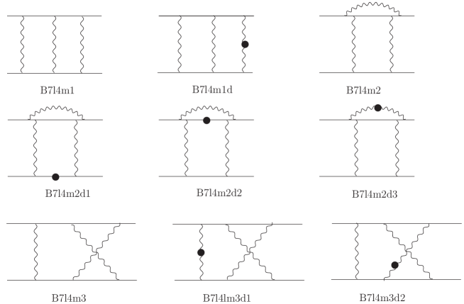
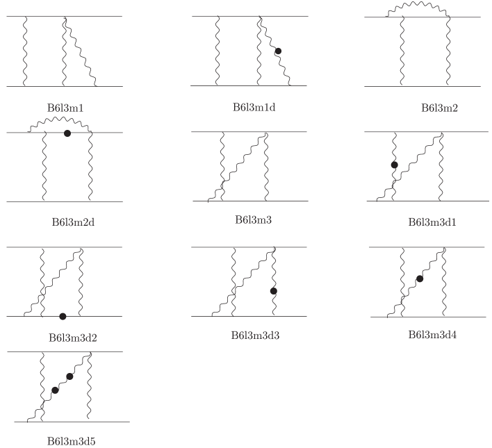
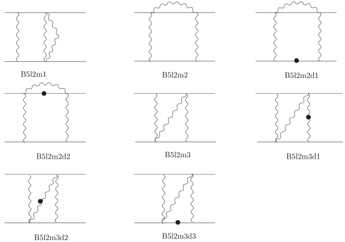
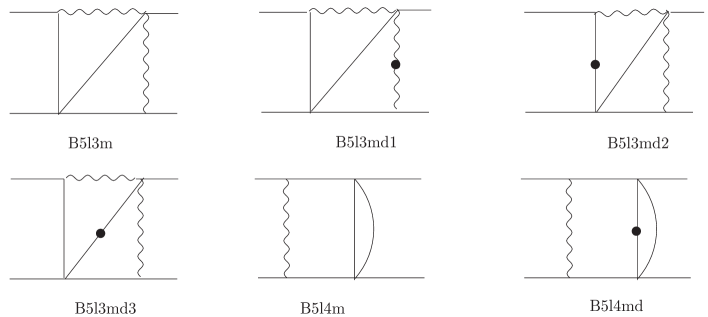
There are thirty three two-loop box MIs. They are shown in Figures 9 to 11. Several analytical expressions for box MIs in terms of HPLs may be found in the file MastersBhabha.m web-masters:2004nn . In Table 4 we list the double-box diagrams to which they contribute. Additionally, one may see the other contributing masters. By now, few of the two-loop box MIs are known analytically. For diagram B1, the MIs B7l4m1 and B7l4m1N are given in Smirnov:2001cm ; for diagram B2, the MI B7l4m2 is known as two-dimensional integral representation Heinrich:2004iq ; for diagram B3, the leading divergent part of MI B7l4m3 is published Heinrich:2004iq . The technique used is the Mellin-Barnes representation Boos:1990rg ; Smirnov:2004ip ; Smirnov:book4 in combination with summation techniques à la Vermaseren:1998uu ; Moch:2001zr ; Moch:2002hm . Other box MIs were derived with systems of differential equations. For diagrams B1 and B3 the MI B5l2m1 has been given in Czakon:2004tg . For diagram B5, a set of two double-box MIs, B5l4m and B5l4mN, was derived recently with the restriction to electrons and photons (one flavor) in Bonciani:2003cj ; web-masters:2004nn . For our set of masters, we use instead of B5l4mN a dotted function:

$${\tt B5l4md} = \frac{-xy}{(1-x^{2})(1-y^{2})}\Bigl{[}\frac{H[0,x]H[0,y]}{\epsilon}+G[-1/y,0,0,x]-G[-y,0,0,x]-\zeta_{2}H[0,x]$$ (41)

$$-~{}4\zeta_{2}H[0,y]+G[-1/y,0,x]H[0,y]+G[-y,0,x]H[0,y]-2H[0,y]H[-1,0,x]$$

$$-6H[0,x]H[-1,0,y]+4H[0,x]H[0,0,y]+G[-1/y,x][3\zeta_{2}+H[0,0,y]]$$

$$-G[-y,x][3\zeta_{2}+H[0,0,y]]+2H[0,x]H[1,0,y]-H[0,0,0,y]\bigr{]}+{\cal O}(\epsilon).$$

The expression depends on HPLs $H$, but also on two-dimensional HPLs $G$ (see Appendix A of Gehrmann:2000zt ; we use here the notations of Bonciani:2003cj and the $G[-y,0,0,x]$ as given in Czakon:2004tg ).

A differential operator for the derivation of differential equations for box diagrams in the $s$-channel is:

$$s\frac{\partial}{\partial s}=\frac{1}{2}\left\{\left(p_{1}^{\mu}+p_{2}^{\mu}\right)+\frac{s\left(p_{2}^{\mu}-p_{3}^{\mu}\right)}{s+t-4}\right\}\frac{\partial}{\partial p_{2}^{\mu}}.$$ (42)

The corresponding operator in the $t$-channel is obtained by the replacements $s\leftrightarrow t$ and $p_{2}\leftrightarrow-p_{3}$. Since the number of differential operators $p_{i}^{\mu}\partial/\partial p_{j}^{\mu}$ is larger than the number of kinematic invariants, there is some freedom of choice. Let us note that representation (42) is much simpler than e.g. that chosen in Bonciani:2003cj .

Figure 9: The nine two-loop box MIs with seven internal lines.

Figure 10: The ten two-loop box MIs with six internal lines.

Figure 11: The fourteen two-loop box MIs with five internal lines.

III.5 Dotted MIs and MIs with irreducible numerators

From the point of view of automatic calculations, there is no essential difference whether a set of MIs is given with or without MIs with irreducible numerators. There exist algebraic relations to transform from one set to the other. However, when the MIs are determined with the help of differential equations, the solution may come out much easier when the unknown MIs are properly chosen. Introducing numerators or dots on lines will change the nature of a MI concerning both the UV and IR singularities. Related to this is that some coupled differential equations for MIs can be decoupled due to separated orders of their $\epsilon$-expansions. Moreover, the solution for a given MI can be much simpler compared to that for another choice. As an example may serve (41), which is by far more compact than the corresponding MI B5l4mN with numerator, given in Equations (37)–(39) of Bonciani:2003cj . Let us also note that the $\epsilon^{2}$ singularity of B5l4mN is absent in (41). Contrary, the masters of prototype SE3l2m web-masters:2004nn are an example for the opposite case where a solution with numerator is simpler than that with a dotted propagator.

Let us finally mention that any of the dotted MIs can be replaced by a MI with an appropriate numerator. However, it is not always possible to “move” a dot arbitrarily from one line to another line. E.g. the dot in V5l2m2d cannot be moved from the massless line to one of the two internal massive lines. The arising integral V5l2m2 [2, 1, 1, 1, 1;0, 0] (defined in (11)) may be considered as a master integral, but cannot replace V5l2m2d. This may be easily proven by the following two algebraic relations:

$${\tt V5l2m2}[1,1,1,2,1;0,0] = {\tt V5l2m2d}-\frac{3(1-5\epsilon+6\epsilon^{2})}{2x(1+2\epsilon)}{\tt V4l1m2}$$ (43)

$$+~{}\frac{3(-1+2\epsilon)(-2+3\epsilon)(-1+3\epsilon)}{4x(-1+2\epsilon+8\epsilon^{2})}{\tt SE3l1m}+\frac{3(2-13\epsilon+27\epsilon^{2}-18\epsilon^{3})}{2\epsilon x^{2}(1+2\epsilon)}{\tt SE3l0m},$$

$${\tt V5l2m2}[2,1,1,1,1;0,0] = -\epsilon~{}{\tt V5l2m2}-\frac{1-5\epsilon+6\epsilon^{2}}{2\epsilon x}{\tt V4l1m2}+\frac{(2-13\epsilon+27\epsilon^{2}-18\epsilon^{3})}{4\epsilon x(1-4\epsilon)}{\tt SE3l1m}.$$ (44)

We conclude for this specific example that the set of masters could be chosen to contain one master out of the pair of integrals with a dot on a massless line ( V5l2m2d, V5l2m2 [1, 1, 1, 2, 1;0, 0]), and one master out of the pair of integrals with no dot or a dot on a massive line ( V5l2m2, V5l2m2 [2, 1, 1, 1, 1;0, 0]).

III.5.1 The divergent parts of the master integrals for the prototypes B5l2m2 and B5l2m3

As was explained in Section III.3.1, under certain conditions one may determine singular parts of MIs in a purely algebraic way or with a combination of algebraic relations and differential equations. We have used this method in order to determine the singularities of the so far unknown MI for prototypes B5l2m2 and B5l2m3:

$${\tt B5l2m2} = \frac{1}{\epsilon}\frac{x}{x^{2}-1}\left(4\zeta_{2}+H[0,0,x]+2H[0,1,x]\right)+{\cal{O}}(1),$$ (45)

$${\tt B5l2m2d1} = -\frac{x}{(1-x)^{2}}\left[\frac{1}{\epsilon^{2}}+\frac{1}{\epsilon}\left(2+H[0,x]+2H[1,x]\right)\right]+{\cal{O}}(1),$$ (46)

$${\tt B5l2m2d2} = {\cal{O}}(1),$$ (47)

$${\tt B5l2m3} = {\cal{O}}(1),$$ (48)

$${\tt B5l2m3d1} = -\frac{1}{\epsilon^{2}}\frac{(1+x^{2})y}{8x(1-y)^{2}}$$ (52)

$$-~{}\frac{1}{\epsilon}\frac{y}{4x(1-y)^{2}(1+y)^{3}}\bigl{[}-(1+x^{2})(1+y)^{3}+\zeta_{2}\left[8(1-x)^{2}(1-y)y\right]$$

$$+~{}2(1+y)\left[x(1-y)^{2}+2y\left(1+x^{2}\right)\right]\left(H[0,y]+2H[1,y]\right)$$

$$-~{}(1-x^{2})(1+y)^{3}H[0,x]+2y(1-x)^{2}(1-y)\left(H[0,0,y]+2H[0,1,y]\right)\bigr{]}+{\cal{O}}(1),$$

$${\tt B5l2m3d2} = -\frac{1}{\epsilon^{2}}\frac{xyH[0,x]}{(1-x^{2})(1-y)^{2}}$$ (53)

$$-~{}\frac{1}{\epsilon}\frac{2xy}{(1-x^{2})(1-y)^{2}}\Bigl{(}H[1,0,x]-H[-1,0,x]+H[0,0,x]$$

$$+~{}\frac{\zeta_{2}}{2}+H[0,x]\left(H[0,y]+2~{}H[1,y]\right)\Bigr{)}+{\cal{O}}(1),$$

$${\tt B5l2m3d3} = -\frac{1}{\epsilon}\frac{y}{2(1-y^{2})}\left[4\zeta_{2}+H[0,0,y]+2H[0,1,y]\right]+{\cal{O}}(1).$$ (54)

III.6 Additional master integrals with several flavors

In QED, there are additional fermion flavors besides electrons. In two-loop Bhabha scattering this leads to the additional diagrams SE5f, V4f, B5f shown in Figure 12. They may be derived from Figures 1 to 3 by a replacement of the closed electron loop in diagrams SE5, V4, B5 by a loop with a second mass scale $M$. As a consequence, additional MIs will arise. We have determined them with DiaGen/IdSolver, and Table 5 lists the MIs which contribute to the evaluation of Feynman integrals of the new prototypes.

Figure 12: The eight additional master integrals with two different mass scales.

IV Summary

The results presented here document a further step towards a complete two-loop prediction of small angle Bhabha scattering, needed e.g. for a precise luminosity determination at the future International Linear Collider.

We have determined a complete set of scalar master integrals needed for the calculation of the virtual two-loop corrections to massive Bhabha scattering in QED, both for one flavor and for several flavors. The MIs are shown pictorially, and we tabulate to which prototype diagrams they will contribute. Further, we determined the first terms of the $\epsilon$-expansions for all the two-loop self-energy and vertex master integrals for the one-flavor case, and some of the two-loop box masters. Some of these master integrals were unknown so far. The analytical expressions are collected in the Mathematica file MastersBhabha.m and are publicly available web-masters:2004nn . As by-products of our numerous tests of the results presented here, we expressed HPLs up to weight 4 by a minimal basis (Mathematica file HPL4.m web-masters:2004nn ), and have generalized the sector decomposition algorithm for the evaluation of Feynman integrals in the Euclidean region to the case of irreducible numerators.

Once the last, most complicated master integrals are determined one will have to combine the virtual two-loop corrections to Bhabha scattering, together with their counter terms, with electroweak corrections and with a package for the treatment of real bremsstrahlung.

Appendix A Numerical evaluation of multi-loop diagrams with irreducible numerators in the Euclidean region

Here we derive expressions for the Feynman integrals $G(X)$ defined in (2) with $L$ loops, a numerator function $X(k_{i})$, N internal lines, and $E$ external legs with momenta $p_{e}$ (see also e.g. Nakanishi:1971 ). The propagator momenta $q_{i}$ compose as:

$$q_{i} = c_{1}^{i}k_{1}+\ldots c_{L}^{i}k_{L}+\ldots+d_{1}p_{1}+\ldots+d_{E}^{i}p_{E}.$$ (55)

In Binoth:2000ps ; Binoth:2003ak , a method was derived for the numerical evaluation of multi-loop Feynman integrals in the Euclidean region. The method is based on sector decomposition (see also Hepp:1966eg ; Roth:1996pd ). In Binoth:2000ps ; Binoth:2003ak , the method was worked out explicitely for propagators only, including dotted ones ($\nu_{i}\neq 1$), i.e. for $X=1$. We need the formulae also with numerators and repeat the starting expression for completeness here, in our notations:

$$G(X) = \frac{1}{(i\pi^{d/2})^{L}}\int\frac{d^{D}k_{1}\ldots d^{D}k_{L}~{}~{}X}{(q_{1}^{2}-m_{1}^{2})^{\nu_{1}}\ldots(q_{j}^{2}-m_{j}^{2})^{\nu_{j}}\ldots(q_{N}^{2}-m_{N}^{2})^{\nu_{N}}}.$$ (56)

The denominator of $G(1)$ contains, after introduction of Feynman parameters $x_{i}$, the momentum dependent function

$$m^{2} = \sum_{i=1}^{N}x_{i}(q_{i}^{2}-m_{i}^{2})~{}=~{}kMk-2kQ+J.$$ (57)

The linear terms in $m^{2}$ may be eliminated by a shift:

$$k = {\bar{k}}+M^{-1}Q,$$ (58)

and the matrix $M$ in (57) may be diagonalized by a rotation:

$$k\to k^{\prime} = V~{}k,$$ (59)

$$kMk = k^{\prime}M_{diag}k^{\prime}$$ (60)

$$\to \sum\alpha_{i}k_{i}^{2},$$ (61)

$$M_{diag} = (V^{-1})^{+}MV^{-1}~{}~{}=~{}(\alpha_{1},\ldots,\alpha_{L}).$$ (62)

After the diagonalization, the momentum integrals may be easily performed, and the remaining Feynman parameter integral contains the term:

$$\frac{(\text{det}~{}M)^{-D/2}}{\left(\mu^{2}\right)^{N_{\nu}-DL/2}} = \frac{U(x)^{N_{\nu}-D(L+1)/2}}{F(x)^{N_{\nu}-DL/2}},$$ (63)

with

$$\mu^{2} = -(J-QM^{-1}Q),$$ (64)

$$N_{\nu} = \nu_{1}+\ldots\nu_{N},$$ (65)

and the definitions :

$$U{(x)} = (\text{det}~{}M),$$ (66)

$$F({x}) = (\text{det}~{}M)\mu^{2}~{}=~{}-(\text{det}~{}M)~{}J+Q\tilde{M}Q.$$ (67)

The $\tilde{M}$ is defined with $M^{-1}=\tilde{M}/\text{det}~{}M$. Finally, one arrives at:

$$G(1) = (-1)^{N_{\nu}}\frac{\Gamma\left(N_{\nu}-\frac{D}{2}L\right)}{\Gamma(\nu_{1})\ldots\Gamma(\nu_{N})}\int_{0}^{1}\prod_{j=1}^{N}dx_{j}~{}x_{j}^{\nu_{j}-1}\delta\left(1-\sum_{i=1}^{N}x_{i}\right)\frac{U(x)^{N_{\nu}-D(L+1)/2}}{F(x)^{N_{\nu}-DL/2}}.$$ (68)

Equation (3) in Binoth:2000ps contains formula (68) for $\nu_{i}=1$.

From the above it is straightforward to formulate the parameter Feynman parameter integrals for the case of nontrivial numerators. The corresponding formulae for the simplest cases are:

$$G(k_{1\alpha}) = (-1)^{N_{\nu}}\frac{\Gamma\left(N_{\nu}-\frac{D}{2}L\right)}{\Gamma(\nu_{1})\ldots\Gamma(\nu_{N})}\int_{0}^{1}\prod_{j=1}^{N}dx_{j}~{}x_{j}^{\nu_{j}-1}\delta\left(1-\sum_{i=1}^{N}x_{i}\right)\frac{{U(x)^{N_{\nu}-1-D(L+1)/2}}}{{F(x)}^{N_{\nu}-DL/2}}\left[\sum_{l}{\tilde{M}}_{1l}Q_{l}\right]_{\alpha},$$

and

$$G(k_{1\alpha}k_{2\beta}) = (-1)^{N_{\nu}}\frac{\Gamma\left(N_{\nu}-\frac{D}{2}L\right)}{\Gamma(\nu_{1})\ldots\Gamma(\nu_{N})}\int_{0}^{1}\prod_{j=1}^{N}dx_{j}~{}x_{j}^{\nu_{j}-1}\delta\left(1-\sum_{i=1}^{N}x_{i}\right)\frac{{U(x)^{N_{\nu}-2-D(L+1)/2}}}{{F(x)}^{N_{\nu}-DL/2}}$$

$$\times\sum_{l}\Biggl{[}[{\tilde{M}}_{1l}Q_{l}]_{\alpha}[{\tilde{M}}_{2l}Q_{l}]_{\beta}-\frac{\Gamma\left(N_{\nu}-\frac{D}{2}L-1\right)}{\Gamma\left(N_{\nu}-\frac{D}{2}L\right)}\frac{g_{\alpha\beta}}{2}{U(x)F(x)}\frac{(V_{1l}^{-1})^{+}(V_{2l}^{-1})}{\alpha_{l}}\Biggr{]}.$$

The general case is treated in Denner:2004iz . Potential UV singularities arise from the overall factors with $\Gamma$ functions and from $U(x)$, while IR singularities arise from $F(x)$. The Mathematica code sectors.m Czakon:2004ww performs the isolation of IR singularities by sector decomposition and the integrations in the Euclidean region. For the numerical calculations the package CUBA Hahn:2004fe is used.

Appendix B Harmonic polylogarithms up to weight 4

The master integrals in the file MastersBhabha.m web-masters:2004nn are expressed by harmonic polylogarithms (HPLs) Remiddi:1999ew up to weight 4. Harmonic polylogarithms fulfill simplified algebraic relations of harmonic sums. One may use this and determine a basis of functions by direct evaluation, and then express the others by algebraic relations. For details we refer to Blumlein:2003gb and references therein.

The three HPLs of weight 1 are:

$$H[0,x] = \ln(x),$$ (71)

$$H[1,x] = -\ln(1-x),$$ (72)

$$H[-1,x] = \ln(1+x).$$ (73)

The nine HPLs of weight 2 may be expressed by three independent HPLs of weight 2 plus those of lower weight:

$$H[0,1,x] = {{\rm{Li_{2}}}}(x),$$ (74)

$$H[0,-1,x] = -{{\rm{Li_{2}}}}(-x),$$ (75)

$$H[-1,1,x] = {{\rm{Li_{2}}}}\left(\frac{1+x}{2}\right)-{{\rm{Li_{2}}}}\left(\frac{1}{2}\right)-\ln 2~{}H[-1,x].$$ (76)

The other HPLs are determined with the relation $H[a,b,x]=-H[b,a,x]+H[a,x]H[b,x]$.

There are 27 HPLs of weight 3 Moch:1999eb , and 8 of them have to be added to the basis: one for each of the six index sets of the class $(a,a,b)$ (see equations (3.22), (3.23) of Blumlein:2003gb ):

$$H[0,0,1,x] = {{\rm{Li_{3}}}}(x),$$ (77)

$$H[0,0,-1,x] = -{{\rm{Li_{3}}}}(-x),$$ (78)

$$H[0,1,1,x] = S_{1,2}(x),$$ (79)

$$H[0,-1,-1,x] = S_{1,2}(-x),$$ (80)

$$H[-1,1,1,x] = S_{1,2}\left(\frac{1+x}{2}\right)-S_{1,2}\left(\frac{1}{2}\right)-\ln 2\left[{{\rm{Li_{2}}}}\left(\frac{1+x}{2}\right)-{{\rm{Li_{2}}}}\left(\frac{1}{2}\right)\right]+\frac{1}{2}\ln^{2}2~{}H[-1,x],$$ (81)

$$H[1,-1,-1,x] = -S_{1,2}\left(\frac{1-x}{2}\right)+S_{1,2}\left(\frac{1}{2}\right)+\ln 2\left[{{\rm{Li_{2}}}}\left(\frac{1-x}{2}\right)-{{\rm{Li_{2}}}}\left(\frac{1}{2}\right)\right]+\frac{1}{2}\ln^{2}2~{}H[1,x],$$ (82)

and two for the class $(a,b,c)$ (see equations (3.7) to (3.10) of Blumlein:2003gb ):

$$H[1,0,-1,x] = \frac{1}{2}S_{1,2}(x^{2})-H[0,1,1,x]-H[0,-1,-1,x]+H[1,x]H[0,-1,x],$$ (83)

$$H[0,-1,1,x] = \int_{0}^{x}\frac{dy}{y}\left[{{\rm{Li_{2}}}}\left(\frac{1+y}{2}\right)-{{\rm{Li_{2}}}}\left(\frac{1}{2}\right)\right]-\ln 2~{}H[0,-1,x].$$ (84)

Further, $H[a,a,a,x]=\frac{1}{6}H[a,x]^{3}$. The integral in (84) may be performed analytically, see $V_{3}(x)$ in (107) or equation (188) in Moch:1999eb .

There are 81 HPLs of weight 4: the three index sets of class $(aaaa)$ have 1 element each (none is basic), the six index sets of class $(aaab)$ have 4 elements each (one is basic), the three index sets of class $(aabb)$ have 6 elements each (one is basic), and the three index sets of class $(aabc)$ have 12 elements each (three are basic). The 18 independent HPLs of weight 4 may be chosen to be:

$$H[0,0,0,1,x] = {{\rm{Li_{4}}}}(x),$$ (85)

$$H[0,0,0,-1,x] = -{{\rm{Li_{4}}}}(-x),$$ (86)

$$H[0,1,1,1,x] = S_{1,3}(x),$$ (87)

$$H[-1,1,1,1,x] = -{{\rm{Li_{4}}}}\left(\frac{1-x}{2}\right)+{{\rm{Li_{4}}}}\left(\frac{1}{2}\right)+\ln(1-x){{\rm{Li_{3}}}}\left(\frac{1-x}{2}\right)-\frac{1}{2}{\ln}^{2}(1-x){{\rm{Li_{2}}}}\left(\frac{1-x}{2}\right)$$ (88)

$$-~{}\frac{1}{6}\ln^{3}(1-x)\ln\frac{1+x}{2},$$

$$H[0,-1,-1,-1,x] = -S_{1,3}(-x),$$ (89)

$$H[1,-1,-1,-1,x] = H[-1,1,1,1,-x],$$ (90)

$$H[0,0,1,1,x] = S_{2,2}(x),$$ (91)

$$H[0,0,-1,-1,x] = S_{2,2}(-x),$$ (92)

$$H[1,1,-1,-1,x] = \int_{0}^{x}\frac{dy}{1-y}H[1,-1,-1,y]$$ (93)

$$= -K_{1}(x)+\ln 2~{}J_{2}(x)+\frac{1}{2}\ln^{2}2~{}H[1,1,x],$$

$$H[-1,0,0,1,x] = \int_{0}^{x}\frac{dy}{1+y}{{\rm{Li_{3}}}}(y),$$ (94)

$$H[-1,0,1,0,x] = -~{}\frac{1}{4}S_{2,2}\left(x^{2}\right)-H[-1,0,0,1,x]+H[0,0,-1,-1,x]+H[0,0,1,1,x]$$ (95)

$$-~{}H[-1,x]H[0,0,1,x]$$

$$+~{}H[0,x](-H[1,x]H[0,-1,x]+H[-1,x]H[0,1,x]+H[1,0,-1,x]),$$

$$H[-1,1,0,0,x] = -\int_{0}^{x}\frac{dy}{1+y}\left[S_{1,2}(1-y)-S_{1,2}(1)\right]$$ (96)

$$= -\ln(1+x)\left[S_{1,2}(1-x)-S_{1,2}(1)\right]-\frac{1}{2}\int_{0}^{x}\frac{dy}{1-y}\ln^{2}(y)\ln(1+y),$$

$$H[0,-1,1,1,x] = U_{4}(x)-\ln 2~{}H[0,-1,1,x]-\frac{1}{2}\ln^{2}2~{}H[0,-1,x],$$ (97)

$$H[0,1,-1,1,x] = -V_{4}(x)-2H[0,-1,1,1,x]+\ln 2~{}\left(H[1,0,-1,x]-H[1,x]H[0,-1,x]\right),$$ (98)

$$H[0,1,1,-1,x] = V_{4}(x)+\frac{1}{2}W_{4}(x)+H[0,-1,1,1,x]-\ln 2~{}\left(H[1,0,-1,x]-H[1,x]H[0,-1,x]\right),$$ (99)

$$H[0,1,-1,-1,x] = -U_{4}(-x)+\ln 2~{}H[0,1,-1,x]-\frac{1}{2}\ln^{2}2~{}H[0,1,x],$$ (100)

$$H[0,-1,1,-1,x] = V_{4}(-x)-2H[0,1,-1,-1,x]-\ln 2~{}\left(H[1,0,-1,x]-H[1,x]H[0,-1,x]\right),$$ (101)

$$H[0,-1,-1,1,x] = -V_{4}(-x)-\frac{1}{2}W_{4}(-x)+H[0,1,-1,-1,x]$$ (102)

$$+~{}\ln 2~{}\left(H[1,0,-1,x]-H[1,x]H[0,-1,x]\right).$$

Further, $H[a,a,a,a,x]=\frac{1}{24}H[a,x]^{4}$. Some auxiliary integrals are defined below in this appendix. The integrals $K_{1}$ and $J_{2}$ in (93) may be performed analytically, see (109) and (110), and that in (96) is not known to us in analytical form. We just mention that the functions with index sets $(0000)$, $(0001)$, $(0011)$, $(0111)$, $(1111)$ may also be found in Gehrmann:2000zt . Our list of HPLs is available in file HPL4.m in web-masters:2004nn . We give here one explicit example of a HPL of the class (aabc), derived with equation (4.26) of Blumlein:2003gb :

$$H[-1,1,0,1,x] = 2H[0,1,1,-1,x]+H[0,1,-1,1,x]+H[1,x](-H[1,-1,0,x]-H[1,0,-1,x]$$ (103)

$$+~{}H[-1,0,1,x]+H[0,-1,1,x])-2H[-1,x]H[0,1,1,x]+H[1,-1,x]H[1,0,x].$$

The above list of functions is a quite compact basis which is sufficient for the computation of all HPLs until weight 4.

For comparisons with Davydychev:2003mv we used additionally to HPLs with arguments $x$ also the following functions:

$$\text{Li}_{n}(x^{2}) = 2^{n-1}\left[H[0,\ldots,0,1,x]-H[0,\ldots,0,-1,x]\right]$$ (104)

with (n-1) zeroes in the arguments, and:

$$S_{1,2}(x^{2}) = H\left[0,1,1,x^{2}\right]=2\left[H[0,1,1,x]-H[0,-1,1,x]-H[0,1,-1,x]+H[0,-1,-1,x]\right],$$ (105)

$$S_{2,2}(x^{2}) = H\left[0,0,1,1,x^{2}\right]=4\left[H[0,0,1,1,x]-H[0,0,-1,1,x]-H[0,0,1,-1,x]+H[0,0,-1,-1,x]\right].$$ (106)

For a study of boundary conditions, one needs the values of HPLs at $x=0$ and $x=1$. Here we follow the algorithms proposed in Remiddi:1999ew .

We have introduced several auxiliary functions. For $H[0,-1,1,x]$ (see (84)) we need:

$$V_{3}(x) = \int_{0}^{x}\frac{dy}{y}\left[{{\rm{Li_{2}}}}\left(\frac{1+y}{2}\right)-{{\rm{Li_{2}}}}\left(\frac{1}{2}\right)\right]$$ (107)

$$= J_{1}(x)+\ln(x)\left[{{\rm{Li_{2}}}}\left(\frac{1+x}{2}\right)-{{\rm{Li_{2}}}}\left(\frac{1}{2}\right)\right]-~{}\ln 2\left[{{\rm{Li_{2}}}}(-x)+\ln(x)\ln(1+x)\right],$$

with

$$J_{1}(x) = \int_{0}^{x}\frac{dy}{1+y}\ln(y)\ln(1-y)$$ (108)

$$= -{{\rm{Li_{3}}}}\left(\frac{1-x}{2}\right)-{{\rm{Li_{3}}}}\left(-x\right)-{{\rm{Li_{3}}}}\left(-\frac{x}{1-x}\right)+{{\rm{Li_{3}}}}\left(-\frac{2x}{1-x}\right)$$

$$+\ln\left(\frac{2x}{1-x}\right)\left[{{\rm{Li_{2}}}}\left(-\frac{x}{1-x}\right)-{{\rm{Li_{2}}}}\left(-\frac{2x}{1-x}\right)\right]+\ln\left(2x\right){{\rm{Li_{2}}}}\left(-x\right)+\ln\left(\frac{1-x}{2}\right){{\rm{Li_{2}}}}\left(\frac{1-x}{2}\right)$$

$$+\frac{1}{2}\ln\left(1-x\right)\left[-\ln 2\ln(1-x)+2\ln 2\ln(2x)+2\ln(x)\ln\left(\frac{1+x}{2}\right)\right]-\left(\frac{1}{3}\ln^{3}2-\frac{7}{8}\zeta_{3}\right).$$

The $H[1,1,-1,-1,x]$ (see (93)) is known analytically, using:

$$K_{1}(x) = \int_{0}^{x}\frac{dy}{1-y}\left[S_{1,2}\left(\frac{1-y}{2}\right)-S_{1,2}\left(\frac{1}{2}\right)\right]$$ (109)

$$= \ln 2~{}J_{3}(x)-\frac{1}{2}K_{2}(x)-\ln(1-x)\left[S_{1,2}\left(\frac{1-x}{2}\right)-S_{1,2}\left(\frac{1}{2}\right)\right]+\frac{1}{4}\ln^{2}2\ln^{2}(1-x),$$

$$J_{2}(x) = \int_{0}^{x}\frac{dy}{1-y}\left[{{\rm{Li_{2}}}}\left(\frac{1-y}{2}\right)-{{\rm{Li_{2}}}}\left(\frac{1}{2}\right)\right]$$ (110)

$$= J_{3}(x)-\ln(1-x)\left[{{\rm{Li_{2}}}}\left(\frac{1-x}{2}\right)-{{\rm{Li_{2}}}}\left(\frac{1}{2}\right)\right]+\frac{1}{2}\ln 2\ln^{2}(1-x),$$

with

$$J_{3}(x) = \int_{0}^{x}\frac{dy}{1-y}\ln(1-y)\ln(1+y)$$ (111)

$$= -{{\rm{Li_{3}}}}\left(\frac{1-x}{2}\right)+{{\rm{Li_{3}}}}\left(\frac{1}{2}\right)+\ln(1-x){\rm{Li_{2}}}\left(\frac{1-x}{2}\right)-\frac{1}{2}\ln 2\ln^{2}(1-x),$$

$$K_{2}(x) = \int_{0}^{x}\frac{dy}{1-y}\ln(1-y)\ln^{2}(1+y)$$ (112)

$$= \frac{7}{10}\zeta_{2}^{2}-\zeta_{2}\ln^{2}2+\ln^{4}2+\frac{1}{4}\ln^{4}(1+x)-\ln^{3}(1+x)\ln(1-x)+\frac{1}{2}\ln^{2}(1+x)\ln^{2}(1-x)$$

$$-\ln 2\ln(1-x)\ln(1+x)\ln\frac{(1-x)}{2(1+x)}-\ln^{3}2~{}\ln\left(1-x^{2}\right)+(\ln^{2}2+\ln^{2}(1-x)){\rm{Li_{2}}}[(1-x)/2]$$

$$+\ln^{2}((1-x)/(1+x)){\rm{Li_{2}}}[-(1-x)/(1+x)]+(\ln^{2}2-\ln^{2}(1+x)){\rm{Li_{2}}}[(1+x)/2]$$

$$-2\ln(1-x){\rm{Li_{3}}}[(1-x)/2]-2\ln[(1-x)/(1+x)]{\rm{Li_{3}}}[-(1-x)/(1+x)]$$

$$+2\ln(1+x){\rm{Li_{3}}}[(1+x)/2]+2{\rm{Li_{4}}}[(1-x)/2]+2{\rm{Li_{4}}}[-(1-x)/(1+x)]-2{\rm{Li_{4}}}[(1+x)/2].$$

In the class $(0,1,1,-1)$ we have an analytical expression for $(H[0,1,1,-1,x]+H[0,1,-1,1,x])$, but not for $H[0,-1,1,1,x]$ and $(H[0,1,1,-1,x]-H[0,1,-1,1,x])$. An analogous statement applies for the class $(0,-1,-1,1)$. The reason is that $W_{4}(x)$ is known from equations (A.28) to (A.33) of reference Davydychev:2003mv :

$$W_{4}(x) = \int_{0}^{x}\frac{dy}{y}\ln^{2}(1-y)\ln(1+y)$$ (113)

$$= -\frac{1}{2}S_{1,3}(x^{2})+2S_{1,3}(-x)-\left[{{\rm{Li_{4}}}}\left(\omega\right)-{{\rm{Li_{4}}}}\left(-\omega\right)\right]+\frac{15}{8}\zeta_{4}$$

$$+~{}\ln(\omega)\left[{{\rm{Li_{3}}}}\left(\omega\right)-{{\rm{Li_{3}}}}\left(-\omega\right)\right]-\frac{1}{2}\ln^{2}(\omega)\left[{{\rm{Li_{2}}}}\left(\omega\right)-{{\rm{Li_{2}}}}\left(-\omega\right)\right]-~{}\frac{1}{6}\ln^{3}(\omega)\ln(x),$$

with $\omega=(1-x)/(1+x)$. By expressing $S_{1,3}(x^{2})$ through HPLs with argument $x$ Remiddi:1999ew , one may derive the remarkably simple relation

$$W_{4}(x)+W_{4}(-x) = -S_{1,3}(x^{2})+2S_{1,3}(x)+2S_{1,3}(-x).$$ (114)

This relation follows also from Davydychev:2003mv .

We have rewritten the two remaining auxiliary functions:

$$U_{4}(x) = \int_{0}^{x}\frac{dy}{y}\left[S_{1,2}\left(\frac{1+y}{2}\right)-S_{1,2}\left(\frac{1}{2}\right)\right]$$ (115)

$$= \ln 2~{}J_{1}(x)-\frac{1}{2}I_{3}(x)+\ln(x)\left[S_{1,2}\left(\frac{1+x}{2}\right)-S_{1,2}\left(\frac{1}{2}\right)\right]$$

$$-\frac{1}{2}\ln^{2}2\left[\ln(x)\ln(1+x)+{\rm{Li_{2}}}(-x)\right],$$

$$V_{4}(x) = \int_{0}^{x}\frac{dy}{y}\ln(1-y)\left[{{\rm{Li_{2}}}}\left(\frac{1+y}{2}\right)-{{\rm{Li_{2}}}}\left(\frac{1}{2}\right)\right]$$ (116)

$$= -I_{2}(x)-{\rm{Li_{2}}}(x)\left[{{\rm{Li_{2}}}}\left(\frac{1+x}{2}\right)-{{\rm{Li_{2}}}}\left(\frac{1}{2}\right)\right]$$

$$+\ln 2\left[\frac{1}{2}S_{1,2}(x^{2})-S_{1,2}(x)-S_{1,2}(-x)+\ln(1+x){\rm{Li_{2}}}(x)\right].$$

We mention finally that we do not know analytical expressions for the following auxiliary functions:

$$I_{1}(x) = \int_{0}^{x}\frac{dy}{1+y}{{\rm{Li_{3}}}}(y),$$ (117)

$$I_{2}(x) = \int_{0}^{x}\frac{dy}{1+y}{\rm{Li_{2}}}(y)\ln(1-y),$$ (118)

$$I_{3}(x) = \int_{0}^{x}\frac{dy}{1+y}\ln(y)\ln^{2}(1-y),$$ (119)

$$I_{4}(x) = \int_{0}^{x}\frac{dy}{1+y}\ln^{2}(y)\ln(1-y).$$ (120)

The first integral is related to $H[-1,0,0,1,x]$ (see (94)), and the next two integrals to four combinations of the six HPLs of classes $(0,a,a,b)$; see (97) to (102) and the remark related to $W_{4}$ before (113). The last one is related to $H[-1,1,0,0,x]$, see (96).

References

• (1) ECFA/DESY LC Physics Working Group Collaboration, J. Aguilar-Saavedra et al., TESLA TDR, Part III: Physics at an $e^{+}e^{-}$ Linear Collider, DESY 2001-011, hep-ph/0106315.
• (2) R. Hawkings and K. Mönig, Eur. Phys. J. direct C1 (1999) 8, hep-ex/9910022.
• (3) H. Abramowicz et al., IEEE Transactions on Nuclear Science 51 (2004) 1.
• (4) FCAL Collaboration, W. Lohmann et al., http://www-zeuthen.desy.de/TESLA/mask/Collaboration.html.
• (5) S. Jadach, hep-ph/0306083.
• (6) S. Jadach, W. Placzek, E. Richter-Was, B. Ward, and Z. Was, Comput. Phys. Commun. 102 (1997) 229–251.
• (7) M. Melles, Acta Phys. Polon. B28 (1997) 1159–1206, hep-ph/9612348.
• (8) A. Arbuzov et al., Nucl. Phys. B485 (1997) 457–502, hep-ph/9512344.
• (9) A. Arbuzov et al., Nucl. Phys. Proc. Suppl. 51C (1996) 154–163, hep-ph/9607228.
• (10) N. Glover, B. Tausk, and J. van der Bij, Phys. Lett. B516 (2001) 33–38, hep-ph/0106052.
• (11) P. Mastrolia and E. Remiddi, Nucl. Phys. B664 (2003) 341–356, hep-ph/0302162.
• (12) R. Bonciani, A. Ferroglia, P. Mastrolia, E. Remiddi, and J. van der Bij, hep-ph/0411321.
• (13) M. Czakon, J. Gluza, and T. Riemann, http://www-zeuthen.desy.de/theory/research/bhabha/.
• (14) G. Passarino, Nucl. Phys. Proc. Suppl. 135 (2004) 265.
• (15) T. Binoth and G. Heinrich, Nucl. Phys. B585 (2000) 741–759, hep-ph/0004013v.2.
• (16) T. Binoth and G. Heinrich, Nucl. Phys. B680 (2004) 375–388, hep-ph/0305234.
• (17) V. Smirnov, Phys. Lett. B524 (2002) 129–136, hep-ph/0111160.
• (18) R. Bonciani, A. Ferroglia, P. Mastrolia, E. Remiddi, and J. van der Bij, Nucl. Phys. B681 (2004) 261–291, hep-ph/0310333.
• (19) G. Heinrich and V. Smirnov, hep-ph/0406053.
• (20) M. Czakon, J. Gluza, and T. Riemann, Nucl. Phys. (Proc. Suppl.) B135 (2004) 83, hep-ph/0406203.
• (21) S. Laporta and E. Remiddi, Phys. Lett. B379 (1996) 283–291, hep-ph/9602417.
• (22) S. Laporta, Int. J. Mod. Phys. A15 (2000) 5087–5159, hep-ph/0102033.
• (23) E. Remiddi, SOLVE, unpublished.
• (24) C. Anastasiou and A. Lazopoulos, JHEP 07 (2004) 046, hep-ph/0404258.
• (25) M. Czakon, DiaGen/IdSolver, unpublished.
• (26) K. Chetyrkin and F. Tkachov, Nucl. Phys. B192 (1981) 159–204.
• (27) T. Gehrmann and E. Remiddi, Nucl. Phys. B580 (2000) 485–518, hep-ph/9912329.
• (28) E. Remiddi and J. Vermaseren, Int. J. Mod. Phys. A15 (2000) 725–754, hep-ph/9905237.
• (29) A. V. Kotikov, Phys. Lett. B259 (1991) 314–322.
• (30) E. Remiddi, Nuovo Cim. A110 (1997) 1435–1452, hep-th/9711188.
• (31) R. Bonciani, P. Mastrolia, and E. Remiddi, Nucl. Phys. B690 (2004) 138–176, hep-ph/0311145.
• (32) R. Bonciani, P. Mastrolia, and E. Remiddi, Nucl. Phys. B661 (2003) 289–343, hep-ph/0301170.
• (33) M. Consoli, Nucl. Phys. B160 (1979) 208.
• (34) M. Böhm, A. Denner, W. Hollik, and R. Sommer, Phys. Lett. B144 (1984) 414.
• (35) M. Böhm, A. Denner, and W. Hollik, Nucl. Phys. B304 (1988) 687.
• (36) D. Bardin, W. Hollik, and T. Riemann, Z. Phys. C49 (1991) 485–490.
• (37) D. Bardin et al., hep-ph/9709229.
• (38) W. Beenakker and G. Passarino, Phys. Lett. B425 (1998) 199–207, hep-ph/9710376.
• (39) D. Bardin et al., Comput. Phys. Commun. 133 (2001) 229–395, hep-ph/9908433.
• (40) Two Fermion Working Group Collaboration, M. Kobel et al., hep-ph/0007180.
• (41) J. Gluza, A. Lorca, and T. Riemann, Nucl. Instrum. Meth. 534 (2004) 289, hep-ph/0409011.
• (42) A. Lorca and T. Riemann, Nucl. Phys. Proc. Suppl. 135 (2004) 328, hep-ph/0407149.
• (43) A. Lorca and T. Riemann, hep-ph/0412047.
• (44) G. ’t Hooft and M. Veltman, Nucl. Phys. B44 (1972) 189–213.
• (45) L. Surguladze and F. Tkachov, Comput. Phys. Commun. 55 (1989) 205–215.
• (46) R. Bonciani. PhD thesis, University of Bologna, 2001.
• (47) J. Fleischer and M. Kalmykov, Comput. Phys. Commun. 128 (2000) 531–549, hep-ph/9907431.
• (48) D. Broadhurst, Z. Phys. C47 (1990) 115–124.
• (49) D. Broadhurst, Z. Phys. C54 (1992) 599–606.
• (50) J. Fleischer, A. Kotikov, and O. Veretin, Nucl. Phys. B547 (1999) 343–374, hep-ph/9808242.
• (51) A. I. Davydychev and M. Y. Kalmykov, Nucl. Phys. B699 (2004) 3–64, hep-th/0303162.
• (52) J. Fleischer, M. Kalmykov and A. Kotikov, Phys. Lett. B462 (1999) 169, hep-ph/9905249.
• (53) M. Czakon, J. Gluza, and T. Riemann, hep-ph/0409017.
• (54) E. Boos and A. Davydychev, Theor. Math. Phys. 89 (1991) 1052–1063.
• (55) V. Smirnov, hep-ph/0406052.
• (56) V. Smirnov, Evaluating Feynman Integrals, vol. 211 of Springer Tracts in Modern Physics. Springer, Berlin, 2004.
• (57) J. Vermaseren, Int. J. Mod. Phys. A14 (1999) 2037–2076, hep-ph/9806280.
• (58) S. Moch, P. Uwer, and S. Weinzierl, J. Math. Phys. 43 (2002) 3363–3386, hep-ph/0110083.
• (59) S. Moch, P. Uwer, and S. Weinzierl, Phys. Rev. D66 (2002) 114001, hep-ph/0207043.
• (60) T. Gehrmann and E. Remiddi, Nucl. Phys. B601 (2001) 248–286, hep-ph/0008287.
• (61) M. Argeri, P. Mastrolia, and E. Remiddi, Nucl. Phys. B631 (2002) 388–400, hep-ph/0202123.
• (62) N. Nakanishi, Graph Theory and Feynman Integrals. Gordon and Breach, 1971.
• (63) K. Hepp, Commun. Math. Phys. 2 (1966) 301–326.
• (64) M. Roth and A. Denner, Nucl. Phys. B479 (1996) 495–514, hep-ph/9605420.
• (65) A. Denner and S. Pozzorini, hep-ph/0408068.
• (66) M. Czakon, sectors.m, unpublished.
• (67) T. Hahn, hep-ph/0404043.
• (68) J. Blümlein, Comput. Phys. Commun. 159 (2004) 19–54, hep-ph/0311046.
• (69) S. Moch and J. Vermaseren, Nucl. Phys. B573 (2000) 853–907, hep-ph/9912355.
• (70) Z. Bern, L. Dixon, and A. Ghinculov, Phys. Rev. D63 (2001) 053007, hep-ph/0010075.
• (71) M. Czakon, J. Gluza, and J. Hejczyk, Nucl. Phys. B642 (2002) 157–172, hep-ph/0205303.
• (72) M. Awramik and M. Czakon, Phys. Rev. Lett. 89 (2002) 241801, hep-ph/0208113.
• (73) M. Czakon, hep-ph/0411261.
• (74) R. H. Lewis, Fermat, http://www.bway.net/~lewis/.
• (75) J. Vermaseren, math-ph/0010025.
• (76) T. Hahn and M. Pérez-Victoria, Comput. Phys. Commun. 118 (1999) 153, hep-ph/9807565.
• (77) T. Hahn, “LoopTools User’s Guide”. http://www.feynarts.de/looptools/.