Radiative $K_{e3}$ decays revisited

Abstract

Motivated by recent experimental results and ongoing measurements, we review the chiral perturbation theory prediction for $K_{L}\to\pi^{\mp}e^{\pm}\nu_{e}\gamma$ decays. Special emphasis is given to the stability of the inner bremsstrahlung-dominated relative branching ratio versus the $K_{e3}$ form factors, and on the separation of the structure-dependent amplitude in differential distributions over the phase space. For the structure-dependent terms, an assessment of the order $p^{6}$ corrections is given, in particular, a full next-to-leading order calculation of the axial component is performed. The experimental analysis of the photon energy spectrum is discussed, and other potentially useful distributions are introduced.

1 Introduction

The amplitude for the semileptonic radiative decays $K_{L}\!\to\pi^{\mp}l^{\pm}\nu_{l}\gamma$ $\left[K_{l3\gamma}\right]$, with $l=e,\mu$, can be divided into two components: the inner bremsstrahlung (IB) that accounts for photon radiation from the external charged particles and which is determined by the non-radiative process $K_{L}\to\pi^{\mp}l^{\pm}\nu_{l}$ $\left[K_{l3}\right]$; and the structure-dependent (SD) amplitude, also called “direct emission”, that describes photon radiation from intermediate hadronic states and represents genuinely new information with respect to the IB one.

Low’s theorem low , applied to $K_{l3\gamma}$, states that the leading contributions in the expansion of the amplitude in powers of the photon four-momentum $q$, namely, the orders $q^{-1}$ and $q^{0}$, are completely determined in a model-independent way by the IB via the $K_{l3}$ form factors and their first order derivatives. The SD amplitude is then defined by the terms of order $q$ and higher. In FFSprl ; FFS , the procedure of low was followed to derive the $q^{-1}$ and $q^{0}$ terms of the IB amplitudes for $K_{l3\gamma}$; moreover, a qualitative, model-dependent, assessment of the SD amplitudes was performed using vector meson dominance. In doncel , the radiative decay modes for both charged and neutral kaons were calculated, taking into account IB terms only. Originally, the main interest was the precision test of soft-photon theorems, allowed by the dominance of IB and the fact that, for $K_{l3\gamma}$, the non-radiative amplitude could in principle be studied extensively and with high accuracy.

Later, $K_{l3\gamma}$ decay amplitudes (including charged kaon ones) were calculated at order $p^{4}$ in chiral perturbation theory (ChPT) in BEG , and branching ratios were evaluated for $l=e,\mu$ in a feasibility study for DAFNE DAFNE . An error analysis and a dedicated study of decay distributions was postponed to a later stage when precise data would become available. It is one of the aims of the present work to provide such an analysis.

ChPT allows for a systematic expansion of transition amplitudes for low momenta of the pseudoscalar mesons wein ; GL . The lowest order amplitude is only of the IB-type with constant $K_{l3}$ form factors, and is independent of free parameters. In addition to providing momentum dependence of the $K_{l3}$ form factors in the bremsstrahlung, the ${\cal O}(p^{4})$ terms predict the existence of non-vanishing SD amplitudes (vector and axial-vector), unambiguously calculable in terms of loop diagrams, low-energy constants of the strong Lagrangian ${\cal L}_{4}$ GL , and the chiral anomaly abb ; wzw . While the anomaly does not require new physical parameters, the low-energy constants are numerically already well-determined from other, independent, meson pro- cesses. Consequently, the experimental verification of the SD amplitude currently represents a significant test of ChPT and, ultimately, of QCD. Of course, since the expansion of the SD amplitudes starts at ${\cal O}(p^{4})$, one may inquire about the role of higher order corrections, a point that will be addressed in the sequel.

In practice, this experimental analysis is complicated by the fact that the radiative $K_{l3}$ branching ratio is largely dominated by the IB, while the SD contribution via IB–SD interference is expected to be an effect at the percent-level (the pure SD rate is negligibly small). On the other hand, the characteristic $q^{-1}$ behavior of the IB by far dominates the lower (and intermediate) photon energy range doncel , while in the upper range where the SD effects become more significant, the number of events is severely reduced. In addition, precise knowledge of the $K_{l3}$ form factors is required for a reliable fit to the photon energy distribution, in order to improve the sensitivity to signals of SD contributions through deviations from the pure IB. All that calls for high precision measurements of both $K_{l3\gamma}$ and $K_{l3}$.

The first measurement of the decay $K_{L}\rightarrow\pi^{\pm}e^{\mp}\nu\gamma$ with significant statistics was performed by the NA31 Collaboration leber in a pioneering experiment, which proved the possibility of precision measurements of this process. Their result for the decay rate relative to $K_{e3}$ decays and for the branching ratio agreed with the theoretical predictions of doncel and BEG , respectively. A few years later, the KTeV Collaboration ktev determined the relative branching ratio, together with the photon spectrum, at percent-level sensitivity. They found a result which is “significantly lower than all published theoretical predictions”. Moreover, from the measured photon energy distribution, two particular combinations of the SD amplitudes were obtained, within rather large uncertainties. Quite recently, new experimental results on $K_{e3\gamma}$ with percent-level accuracy have been presented by the NA48 na48 and by the KTeV ktev_04 Collaborations, respectively.

The experimental situation has therefore become quite promising and clearly justifies renewed interest in radiative $K_{e3}$ decays. In this regard, particularly relevant topics are the stability of IB with respect to the $K_{e3}$ form factor parameterizations, the separation itself of the radiative amplitude into IB and SD contributions and the re-visitation the ChPT calculation of the SD component, including in particular next-to-leading ${\cal O}(p^{6})$ corrections. Moreover, this represents an opportunity to discuss, besides the photon spectrum, also other differential distributions that may help in the study of the SD terms in high statistics experiments.

In the sequel, we limit our consideration to the $K_{e3\gamma}$ transition, since current experimental data with appropriate statistics refer to this mode only. Specifically, in Sects. 2 and 3 we review the experimental situation and the experimental observables, the kinematics, and the amplitude definitions with particular emphasis on the separation into IB and SD contributions. In Sect. 4 we present the ChPT results for the SD amplitudes, notably the ${\cal O}(p^{6})$ corrections for the axial amplitudes. In Sect. 5 we numerically discuss the relative radiative branching ratio, while Sects. 6 and 7 are devoted to numerical estimates of the SD amplitudes, the photon energy distribution and the comparison with experimental results. Also, other kinds of differential distributions are discussed there. Finally, Sect. 8 contains a summary of the results, while details of the calculations are collected in the appendices.

2 Experimental status and observables

As already mentioned, we concentrate on $K_{e3\gamma}$ decays where high statistics experimental data on the branching ratio and photon energy spectrum have become available. For a presentation of the experimental status in the other channels, we refer the reader to the PDG listing PDG .

Measuring the decay rate relative to $K_{e3}$ is much safer than absolute measurements, as the former is free from uncertainties related to experimental normalizations, calibrations, and machine luminosity. Basically, an inclusive $K_{e3}$ sample of events is collected, all characterized by one lepton and one pion of opposite charges emitted from a common vertex, without any restriction on the number of emitted photons. A radiative $K_{e3\gamma}$ subsample is extracted by imposing additional criteria dictated by the apparatus and the experimental conditions, in particular by the request of having at least one hard photon in each of those events.

To achieve optimal identification of the candidate $K_{e3\gamma}$ events, kinematical cuts are applied to the radiative sample. In particular, thresholds in the photon energy and in the photon–electron opening angle are usually imposed, see, e.g., doncel . Then, the experimental results generally concern the relative branching ratio

$$R\left(E_{\gamma}^{\rm cut},\,\theta_{e\gamma}^{\rm cut}\right)\,=\,\frac{\Gamma\left(K_{e3\gamma},\,E_{\gamma}^{*}>E_{\gamma}^{\rm cut},\,\theta_{e\gamma}^{*}>\theta_{e\gamma}^{\rm cut}\right)}{\Gamma\left(K_{e3}\right)}~{},$$ (2.1)

where $E_{\gamma}^{*}$ and $\theta_{e\gamma}^{*}$ indicate the photon energy and the photon–electron opening angle in the kaon rest frame, respectively.

From the above, the measured value of $R$ is determined by the ratio of the number of events in the $K_{e3\gamma}$ and $K_{e3}$ samples, each divided by the respective experimental acceptances. The available experimental results are displayed in Table 1.

Table 1: Experimental values of $R$ for the transition $K_{e3\gamma}$. The first error is statistical, the second one systematic.

${\rm Ref.}$	$E_{\gamma}^{\rm cut}$	$\theta_{e\gamma}^{\rm cut}$	events	$R\times 10^{2}$
na48	$30\hskip 3.0pt{\rm MeV}$	$20^{\circ}$	$18977$	$\,0.964\;\pm 0.008\;^{+~{}0.011}_{-~{}0.009}~{}$
ktev_04	$30\,{\rm MeV}$	$20^{\circ}$	$4309$	$0.916\pm 0.017$
ktev_04	$10\,{\rm MeV}$	$0^{\circ}$	$14221$	$\,4.942\;\pm 0.042\pm 0.046$
ktev	$30\,{\rm MeV}$	$20^{\circ}$	$15463$	$\,0.908\;\pm 0.008\;^{+~{}0.013}_{-~{}0.012}~{}$
leber	$30\,{\rm MeV}$	$20^{\circ}$	$1384$	$\,0.934\;\pm 0.036\;^{+~{}0.055}_{-~{}0.039}~{}$
peach	$15\,{\rm MeV}$	$0^{\circ}$	$10$	$\,3.3\;\pm 2.0$

One may notice that the KTeV 04 result for $R$ ktev_04 with angular cuts is based on a much smaller number of $K_{e3\gamma}$ events with respect to their previous determination ktev , yet the achieved uncertainty based on their more recent data is comparable owing to a much reduced systematic uncertainty.

As regards the photon energy distribution, one can investigate the spectrum with free normalization because the essential features lie exclusively in the shape. Indeed, structure-dependent emission should manifest itself in the harder portion of the photon energy spectrum, via a modification of the pure IB spectrum which is controlled by the $K_{e3}$ form factors. An attempt along these lines was made by the KTeV 01 experiment ktev , which used a simplified decomposition of the structure-dependent amplitude, and their analysis will be commented upon in the sequel. This is the only experimental information on structure-dependent emission currently available, as neither NA48 nor KTeV have so far presented an analysis of this point based on the more recent data.

As far as the perspectives of $K^{\pm}_{e3\gamma}$ measurements are concerned that may complement the currently available data for $K_{e3\gamma}$, new results on these transitions are expected from the NA48 experiment NA48private . In the more remote future, substantially increased statistics for $K^{\pm}_{l3\gamma}$ decays should be expected in connection with the construction of higher intensity kaon beams, with accumulated samples of $10^{6}$ (or more) candidate events landsberg .

3 The decay amplitude

In the following, we consider the decay

$$K^{0}(p) \to \pi^{-}(p^{\prime})\,e^{+}(p_{e})\,\nu_{e}(p_{\nu})\,\gamma(q)\qquad[K_{e3\gamma}^{0}]$$ (3.1)

and its charge conjugate mode. We disregard $CP$-violating contributions, and study the emission of a real photon ($q^{2}=0$).

3.1 The matrix element

The transition matrix element has the form

$$\begin{split}T(K_{e3\gamma}^{0})&\,=\,\frac{G_{F}}{\sqrt{2}}\,e\,V^{*}_{us}\,\epsilon^{\mu}(q)^{*}\biggl{[}\bigl{(}V_{\mu\nu}-A_{\mu\nu}\bigr{)}\times\\ &\hskip 99.58464pt\times\bar{u}(p_{\nu})\,\gamma^{\nu}\,(1-\gamma_{5})\,v(p_{e})\\ &\,+\,\frac{F_{\nu}}{2p_{e}q}\,\bar{u}(p_{\nu})\,\gamma^{\nu}\,(1-\gamma_{5})\,\bigl{(}m_{e}-\not\!p_{e}-\not\!q\bigr{)}\,\gamma_{\mu}\,v(p_{e})\biggr{]}\\ &\,\doteq\,\epsilon^{\mu}(q)^{*}M_{\mu}~{}.\end{split}$$ (3.2)

The relevant diagrams are displayed in Fig. 1.

Figure 1: Diagrams describing $K_{l3\gamma}^{0}$ decay

The first term of (3.2) corresponds to diagram a), which includes bremsstrahlung off the charged pion, while the second one corresponds to the radiation off the positron, represented by the diagram b). We have introduced the hadronic tensors $V_{\mu\nu}$ and $A_{\mu\nu}$,

$$\begin{split}I_{\mu\nu}&\,=\,i\,\int d^{4}x\,e^{iqx}\,\langle\pi^{-}(p^{\prime})|T\,V^{\rm em}_{\mu}(x)\,I^{\rm had}_{\nu}(0)|K^{0}(p)\rangle~{}\,;\,\\ \quad I&\,=\,V,A~{},\end{split}$$ (3.3)

whereas $F_{\mu}$ is the $K_{l3}$ matrix element

$$F_{\mu}\,=\,\langle\pi^{-}(p^{\prime})|V^{\rm had}_{\mu}(0)|K^{0}(p)\rangle~{}\,,\,$$ (3.4)

with

$$\begin{split}V_{\mu}^{\rm had}&\,=\,\bar{s}\gamma_{\mu}u~{},~{}~{}A_{\mu}^{\rm had}\,=\,\bar{s}\gamma_{\mu}\gamma_{5}u~{},\\ V^{\rm em}_{\mu}&\,=\,\bigl{(}2\bar{u}u-\bar{d}d-\bar{s}s\bigr{)}/3~{}.\end{split}$$ (3.5)

The tensors $V_{\mu\nu}$ and $A_{\mu\nu}$ satisfy the Ward identities

$$\begin{split}q^{\mu}V_{\mu\nu}&\,=\,F_{\nu}~{},\\ q^{\mu}A_{\mu\nu}&\,=\,0~{},\end{split}$$ (3.6)

which imply gauge invariance of the total amplitude (3.2),

$$q^{\mu}M_{\mu}\,=\,0~{}.$$ (3.7)

3.2 Inner bremsstrahlung, structure-dependent
terms and all that

Low’s theorem is employed in FFS to obtain the IB amplitude for $K_{l3\gamma}$ decays, written entirely in terms of the $K_{l3}$ form factors and their derivatives. In this subsection we present an alternative way of separating the amplitude into an IB and a SD part that directly starts from the following two requirements:

1. In order to describe two different physical mechanisms, the IB and SD amplitudes must be separately gauge invariant.

2. The SD amplitude contains terms of order $q$ and higher.

The second condition does not prevent the IB amplitude from containing terms of order $q$ and higher. Splitting the amplitude under this less restrictive condition allows one to put more terms into the IB part, still using only the non-radiative matrix element in this part of the amplitude. This has the advantage that one can make more precise predictions for the decay process, as we will see below.

The splitting of the transition amplitude $T$ into an IB and a SD part requires a corresponding splitting of the hadronic tensor $I_{\mu\nu}$. Consider first the axial correlator. There are no contributions where the photon is emitted from the pion line. Therefore, $A_{\mu\nu}$ is considered to be a purely SD contribution. It can be written in the form BEG

$$\begin{split}A_{\mu\nu}&\,=\,A_{\mu\nu}^{\rm SD}\\ &\,=\,i\,\epsilon_{\mu\nu\rho\sigma}\,\bigl{(}A_{1}\,p^{\prime\rho}q^{\sigma}+A_{2}\,q^{\rho}W^{\sigma}\bigr{)}\\ &\hskip 12.80365pt+i\,\epsilon_{\mu\lambda\rho\sigma}\,p^{\prime\lambda}q^{\rho}W^{\sigma}\,\bigl{(}A_{3}\,W_{\nu}+A_{4}\,p^{\prime}_{\nu}\bigr{)}~{},\end{split}$$ (3.8)

where $W_{\mu}=(p-p^{\prime}-q)_{\mu}$. (We use the convention $\epsilon_{0123}=+1$.) The amplitude is manifestly of order $q$ and higher, because the $A_{i}$ are non-singular at zero photon energy. The Lorentz invariant components $A_{i}$ depend on three independent scalar variables that can be built from $p,\,p^{\prime}$, and $q$ – we come back on this in the following paragraph.

The decomposition of the vector correlator reads

$$V_{\mu\nu}=V^{\rm IB}_{\mu\nu}+V^{\rm SD}_{\mu\nu}~{}\,,\,$$ (3.9)

where the IB piece is chosen such that

$$q^{\mu}V_{\mu\nu}^{\rm IB}=F_{\nu}(t)~{}\,,\,$$ (3.10)

as a result of which we have

$$q^{\mu}V_{\mu\nu}^{\rm SD}=0~{}\,.\,$$ (3.11)

The structure-dependent part of the decay amplitude $T$ in (3.2) is defined to be

$$\begin{split}T^{\rm SD}&\,=\,\frac{G_{F}}{\sqrt{2}}\,e\,V^{*}_{us}\,\epsilon^{\mu}(q)^{*}\left(V_{\mu\nu}^{\rm SD}-A_{\mu\nu}^{\rm SD}\right)\times\\ &\hskip 71.13188pt\times\bar{u}(p_{\nu})\,\gamma^{\nu}\,(1-\gamma_{5})\,v(p_{l})~{},\end{split}$$ (3.12)

whereas the bremsstrahlung part is $T^{\rm IB}=T-T^{\rm SD}$.

It remains to explicitly construct the decomposition (3.9). In order not to interrupt the argument, we refer the interested reader to Appendix E and simply display here the result,

$$V_{\mu\nu}^{\rm IB} \,=\,\frac{p^{\prime}_{\mu}}{p^{\prime}q}\bigl{(}2p_{\nu}f_{+}(W^{2})-W_{\nu}f_{2}(W^{2})\bigr{)}$$

$$\,+\frac{W_{\mu}}{qW}\bigl{(}2(p-q)_{\nu}\triangle f_{+}-W_{\nu}\triangle f_{2}\bigr{)}$$ (3.13)

$$\,+g_{\mu\nu}\bigl{(}2\triangle f_{+}-f_{2}(t)\bigr{)}~{}\,,\,$$

$$\triangle f_{i} \,=\,f_{i}(t)-f_{i}(W^{2})~{}\,,\,~{}i=+,2~{}\,,\,$$ (3.14)

where $f_{+},\,f_{2}$ are the form factors (3.4)

$$F_{\mu}=2p_{\mu}f_{+}(t)+(p^{\prime}-p)_{\mu}f_{2}(t)~{}\,,\,~{}t=(p-p^{\prime})^{2}~{}\,.\,$$ (3.15)

We use the form factors $f_{+},\,f_{2}$ instead of the usual $f_{+}$, $f_{-}=f_{+}-f_{2}$ ones for easier comparison with the work of FFS .

The IB part derived in FFS differs from the one used here through terms of order $q$. It can be obtained from $V_{\mu\nu}^{\rm IB}$ by subtracting all terms of order $q$ and higher from the latter, and merging them into the SD part of the amplitude. Because the terms to be subtracted can be expressed through the form factors $f_{+},\,f_{2}$ and their derivatives, we believe that it does not make much sense to perform this purification of the IB part, and we will mostly stick with the convention (3.13). While comparing with the KTeV result ktev , we will have the occasion to compare (3.13) with the conventional decompositions FFS in more detail in Sect. 6.3.

Let us shortly discuss the salient features of the IB term (3.13). First, it satisfies the Ward identity (3.10). Second, it contains all infrared singular pieces proportional to $1/p^{\prime}q$. With this we mean the following. The residue of the singularity is a non-trivial function of the momenta $p$, $p^{\prime}$, $q$. The decomposition (3.13) takes into account all singularities at $p^{\prime}q=0$, in contrast to the standard treatment FFS , which considers e.g. a term like $(qW)^{2}/p^{\prime}q$ to be of order $q$, to be relegated to the SD part of the amplitude.

It is useful to decompose also the SD part of the vector amplitude into a set of gauge invariant tensors. In the following, we often use the basis proposed in poblaguev ,

$$\begin{split}V_{\mu\nu}^{\rm SD}&\,=\,V_{1}\bigl{(}p^{\prime}_{\mu}q_{\nu}-p^{\prime}\!q\,g_{\mu\nu}\bigr{)}+V_{2}\bigl{(}W_{\mu}q_{\nu}-qWg_{\mu\nu}\bigr{)}\\ &\hskip 12.80365pt+V_{3}\bigl{(}qWp^{\prime}_{\mu}W_{\nu}-p^{\prime}\!q\,W_{\mu}W_{\nu}\bigr{)}\\ &\hskip 12.80365pt+V_{4}\bigl{(}qWp^{\prime}_{\mu}p^{\prime}_{\nu}-p^{\prime}\!q\,W_{\mu}p^{\prime}_{\nu}\bigr{)}~{}.\end{split}$$ (3.16)

The Lorentz invariant amplitudes $V_{i}$ again depend on the 3 scalars that can be formed from $p$, $p^{\prime}$, and $q$.

3.3 Kinematics

It remains to shortly recall the kinematics of this decay, and we begin with the Lorentz invariant amplitudes $A_{i},V_{i}$. As already mentioned, these are functions of three scalar variables that we often take to be

$$s\,=\,(q+p^{\prime})^{2}~{},~{}~{}t\,=\,(p-p^{\prime})^{2}~{},~{}~{}u\,=\,(p-q)^{2}~{}.$$ (3.17)

These variables are useful in the discussion of the analytic properties of $V_{i},A_{i}$. In (3.3), the variables $s$, $t$, $u$ can assume any value, whereas the physical region in $K_{e3\gamma}$ decays can be represented as follows. For fixed $W^{2}$, the variables $s$, $t$, and $u$ vary in

$$W^{2} \,\leq\,t\,\leq\,(M_{K}-M_{\pi})^{2}~{},$$

$$s_{-} \,\leq\,s\,\leq\,s_{+}~{},$$

$$s_{\pm} \,=\,M_{\pi}^{2}-\frac{1}{2t}(t+M_{\pi}^{2}-M_{K}^{2})(t-W^{2})$$

$$\,\pm\,\frac{1}{2t}\lambda^{1/2}(t,M_{K}^{2},M_{\pi}^{2})\lambda^{1/2}(t,0,W^{2})~{},$$

$$s+t+u \,=\,M_{K}^{2}+M_{\pi}^{2}+W^{2}~{},$$ (3.18)

where

$$\lambda(x,y,z)\,=\,x^{2}+y^{2}+z^{2}-2(xy+xz+yz)~{}.$$ (3.19)

Varying the invariant mass squared $W^{2}$ of the lepton pair in the interval

$$m_{e}^{2}\,\leq\,W^{2}\,\leq\,(M_{K}-M_{\pi})^{2}$$ (3.20)

generates the region covered by $s,t,u$ in $K_{l3\gamma}$ decays. In Sect. 4.2, where the analytic properties of the amplitudes $A_{i},\,V_{i}$ are discussed, we display the region (3.18) in the Mandelstam plane.

Instead of $s,t,u$, we also use

$$pq/M_{K}\,=\,E_{\gamma}^{*}~{},\quad pp^{\prime}/M_{K}\,=\,E_{\pi}^{*}~{},\quad W^{2}\,=\,(p_{l}+p_{\nu})^{2}~{},$$ (3.21)

where $E_{\gamma}^{*},~{}E_{\pi}^{*}$ are the photon and the pion energy in the kaon rest frame. This set is useful when discussing partial decay widths.

In the case of four body decays we have five independent variables, thus two more variables are needed to describe fully the kinematics of $K_{l3\gamma}$ decays. We choose

$$pp_{e}/M_{K}\,=\,{E_{e}^{*}}~{},\quad x\,=\,p_{e}q/M_{K}^{2},$$ (3.22)

where ${E_{e}^{*}}$ is the positron energy in the kaon rest frame. The dimensionless variable $x$ is related to the angle $\theta_{e\gamma}^{*}$ between the photon and the positron:

$$xM_{K}^{2}\,=\,E_{\gamma}^{*}\,\left({E_{e}^{*}}-\sqrt{{E_{e}^{*}}^{2}-m_{e}^{2}}\,\cos\theta_{e\gamma}^{*}\right).$$ (3.23)

The total decay rate is given by

$$\Gamma(K^{0}\to\pi^{-}e^{+}\nu\gamma)\,=\,$$ (3.24)

$$\hskip 28.45274pt\frac{1}{2M_{K}(2\pi)^{8}}\,\int d_{\rm LIPS}(p;\,p^{\prime},p_{e},p_{\nu},q)\,\sum_{\rm spins}\left|T\right|^{2}~{},$$

where $T$ is the amplitude in (3.2), and we denote the Lorentz invariant phase space element for the $K_{l3\gamma}$ process by $d_{\rm LIPS}(p;\,p^{\prime},p_{e},p_{\nu},q)$. The square of the matrix element (3.2), summed over photon and lepton polarizations, is a bilinear form in the invariant amplitudes $V_{i},A_{i},f_{+}$ and $f_{2}$. Performing the traces over the spins, we work with massless spinors, as a result of which the form factors $A_{3},V_{3}$ and $f_{2}$ drop out in the final expressions. [The electron mass cannot be set to zero everywhere, because the IB part of the transition amplitude contains mass singularities, generated by the diagram Fig. 1b.] In Appendix B, we display the explicit result for $\sum_{\rm spins}\left|T\right|^{2}$, in particular the $T$-odd terms that are generated by the imaginary parts of the structure functions, and comment on the relation to the width of $K_{L}$.

4 Analytical results from ChPT

While Low’s theorem furnishes a recipe to evaluate the terms of order $1/q$ and $q^{0}$ of an amplitude associated with a general radiative process, it does not give any insight into the terms of order $q$ and higher, that is the SD part. A convenient tool to derive expressions for the SD amplitude is ChPT. For the axial part, ChPT directly generates the corresponding amplitude in a series expansion in the momenta, the leading contribution is generated by the Wess-Zumino-Witten (WZW) term wzw . As for the vector amplitude, the chiral expansion contains both IB and SD terms, hence if one simultaneously evaluates the $K_{l3}$ matrix element, the decomposition (3.13) leads to the chiral expansion of the SD term.

4.1 ChPT results at order $p^{4}$

In BEG , the chiral expansion was carried out up to ${\cal O}(p^{4})$ for the neutral and for the charged decay modes. [A tree-level calculation up to this order without the loop contributions was performed in holstein .] We do not describe the calculation here and refer the interested reader to the original article. The result for the SD terms is as follows. For the axial amplitude, one has

$$A_{2}=-\frac{1}{8\pi^{2}F^{2}}~{},~{}~{}A_{1}=A_{3}=A_{4}=0~{}~{}[{\cal O}(p^{4})]~{}.$$ (4.1)

$F$ is the pion decay constant in the chiral limit. We display the result for the vector amplitude $V_{\mu\nu}^{\rm SD}$ in terms of the Lorentz invariant form factors $V_{i}$,

$$\begin{split}V_{1}&=\sqrt{2}\,\tilde{I}_{2}~{},\\ V_{2}&=\frac{\sqrt{2}}{qW}\left(\tilde{I}_{1}-p^{\prime}q\,\tilde{I}_{2}+\sqrt{2}\triangle f_{+}\right)~{},\\ V_{3}&=\frac{\sqrt{2}}{qW}\left(\tilde{I}_{3}-\tilde{f}_{2}^{+}(W^{2})\right)~{},\\ V_{4}&=0\hskip 28.45274pt[{\cal O}(p^{4})]~{}.\end{split}$$ (4.2)

The integrals $\tilde{I}_{i},\,\tilde{f}_{2}^{+}$ are defined as follows. In BEG , the one-loop expression for $V_{\mu\nu}$ in the charged decay mode $K^{+}_{l3\gamma}$ is defined in terms of integrals $I_{i},\,f_{i}^{+}$, explicitly displayed there. The quantities $\tilde{I}_{i},\,\tilde{f}_{2}^{+}$ are obtained from $I_{i},\,f_{2}^{+}$ by

1. replacing the arguments $(p,p^{\prime})$ by $-(p^{\prime},p)$ in the $I_{i}\,$;

2. inserting the appropriate coefficients $c_{i}^{I}$ for $K^{0}_{l3\gamma}$ listed in Table 10 of that reference.

Note in addition that $\triangle f_{+}$ in (4.2) refers to the chiral one-loop representation of this quantity.

It turns out that the form factors $V_{i}$ are nearly constant over the physical phase space. This is due to the fact that in the vicinity of the physical phase space, there are no singularities at this order in the chiral expansion. This fact allows one to derive expressions for the SD parts that are considerably simpler than the full ones, yet still precise enough for our purpose. In a first step, we expand these amplitudes in powers of the photon momentum $q$ and keep only the leading order term. This amounts to setting $s=M_{\pi}^{2},u=M_{K}^{2}$, as a result of which the $V_{i}$ become functions of $t$ alone. It turns out that all loop integrals can be expressed in terms of the standard one-loop integral $\bar{J}(t)$. The resulting expressions are displayed in Appendix C. An even more drastic simplification results when one furthermore sets $t=0$ in the simplified formulae. The result reads

$$V_{1} =-\frac{8}{F^{2}}\bar{L}_{9}-\frac{(1-x)^{-2}}{32\pi^{2}F^{2}}\biggl{\{}\frac{1}{3}\left(53-25x+2x^{2}\right)$$

$$\hskip 12.80365pt+\left(1+x-x^{2}+x^{3}\right)\frac{\log x}{2(1-x)}$$

$$\hskip 12.80365pt-\left(127-93x+21x^{2}-x^{3}\right)\frac{\log y}{2(1-x)}\biggr{\}}+{\cal O}(q,t)~{},$$

$$V_{2} =\frac{4}{F^{2}}\left(\bar{L}_{9}+\bar{L}_{10}\right)$$

$$\hskip 12.80365pt+\frac{(1+x)(1-x)^{-2}}{64\pi^{2}F^{2}}\biggl{\{}1+x+\frac{2x\log x}{1-x}\biggr{\}}$$

$$\hskip 12.80365pt-\frac{(1-x)^{-3}}{32\pi^{2}F^{2}}\biggl{\{}\frac{166}{3}(9-4x)+(77-x)\frac{x^{2}}{3}$$

$$\hskip 12.80365pt+x(3+2x)\frac{\log x}{1-x}-9(12-x)(4-x)^{2}\frac{\log y}{1-x}\biggr{\}}$$

$$\hskip 12.80365pt+{\cal O}(q,t)~{},$$

$$V_{3} =-\frac{(1-x)^{-4}}{32\pi^{2}F^{2}M_{K}^{2}}\biggl{\{}\frac{2611}{3}-13x(34-5x)-\frac{4}{3}x^{3}$$

$$\hskip 12.80365pt+x(2+3x+x^{2})\frac{\log x}{1-x}-27(7-x)(4-x)^{2}\frac{\log y}{1-x}\biggr{\}}$$

$$\hskip 12.80365pt+{\cal O}(q,t)~{}.$$ (4.3)

Here, $x=M_{\pi}^{2}/M_{K}^{2}$, $y=M_{\eta}^{2}/M_{K}^{2}$. Furthermore, it is understood that $M_{\eta}^{2}$ is related to $M_{K}^{2},M_{\pi}^{2}$ through the Gell-Mann–Okubo relation.

4.2 ChPT results at order $p^{6}$

There are two main reasons to consider ${\cal O}(p^{6})$ corrections to the structure-dependent terms as described in the previous subsection:

1. As the structure-dependent terms vanish at tree level in the chiral expansion, the one-loop or ${\cal O}(p^{4})$ predictions are only the leading order results for these amplitudes. Subleading corrections are often sizeable in chiral SU(3), therefore it is mandatory to investigate ${\cal O}(p^{6})$ terms in order to be sure to control the size of the structure-dependent terms. Furthermore, several of the structure functions vanish at leading (one-loop) order ($V_{4}$, $A_{1}$, $A_{3}$, $A_{4}$) or nearly so in the sense that they do not allow for natural-size counterterms ($V_{3}$), so the size of corrections to these is completely unknown from the one-loop results.

2. At ${\cal O}(p^{4})$, all structure functions are real in the physical region, and the cuts in these functions lie far outside the kinematically allowed range. This is the reason why they are so smooth and can be approximated to such high accuracy by simple polynomials. However, this changes at ${\cal O}(p^{6})$, as will be seen below.

For the following discussion, we again use the Mandelstam variables $s$, $t$, $u$. The lowest-lying cuts for the structure functions in terms of these three variables are as follows:

1. For the weak vector current, they start at $s_{\rm thr}=9M_{\pi}^{2}$, $t_{\rm thr}=(M_{K}+M_{\pi})^{2}$, $u_{\rm thr}=(M_{K}+2M_{\pi})^{2}$, respectively. Only the $t$-channel cut exists at ${\cal O}(p^{4})$ as the other two require three-particle intermediate states and therefore occur only at two-loop order.

2. For the weak axial current, cuts start at $s_{\rm thr}=4M_{\pi}^{2}$, $t_{\rm thr}=(M_{K}+M_{\pi})^{2}$, $u_{\rm thr}=(M_{K}+M_{\pi})^{2}$, respectively. All these occur at one-loop order, but are suppressed to ${\cal O}(p^{6})$ as they require an anomalous vertex.

Figure 2: Cuts in the complex plane for the vector (left panel) and axial (right panel) amplitudes for fixed $W^{2}=m_{e}^{2}$. The arrows indicate the part of the plane where the decay amplitude is complex, starting from the lowest cuts indicated by the full lines. The limits of physical phase space are also shown (thick solid line).

These cuts are displayed graphically in Fig. 2, where we have drawn them in the Mandelstam plane together with the allowed phase space for fixed (and minimal) $W^{2}=m_{e}^{2}$, which corresponds to the maximal range in $s$, $t$, $u$. While the $t$- and $u$-channel cuts lie far outside the physical region, we note that the $s$-channel cuts overlap with it (precisely: for $W^{2}<(M_{K}-3M_{\pi})^{2}$ in the vector and $W^{2}<(M_{K}-2M_{\pi})^{2}$ in the axial case), such that at least some of the structure functions become complex at ${\cal O}(p^{6})$.

Figure 3: Feynman diagrams with cuts for a) $s>4M_{\pi}^{2}$, b) $s>9M_{\pi}^{2}$, c) $t>(M_{K}+M_{\pi})^{2}$, respectively. The filled vertex denotes a contribution from the anomalous Lagrangian at order $p^{4}$. The first two diagrams provide the structure functions with imaginary parts in the physical region, while the last one generates the only cut present in the amplitudes at ${\cal O}(p^{4})$.

The diagrams with cuts responsible for imaginary parts in the physical region are displayed in Fig. 3, together with one typical diagram for the $t$-channel cut appearing at ${\cal O}(p^{4})$. Due to the smallness of phase space for the three-pion intermediate state, we expect the effect of the cut in the vector structure functions to be tiny.

For the above considerations, we have regarded $W^{2}$ as a fixed “mass squared” of the lepton-neutrino pair, which is of course not true. There are additional cuts in $W^{2}$, the lowest one starting at $W^{2}=(M_{K}+M_{\pi})^{2}$ present at one loop, but sufficiently far outside the physical region, plus a pole at $W^{2}=M_{K}^{2}$ that however only appears in the structure function $A_{3}$. The pole at $s=M_{\pi}^{2}$ defines the bremsstrahlung part and is not present in the structure-dependent terms as defined by our convention.

4.2.1 Complete order $p^{6}$ corrections to the axial amplitudes

We have calculated the complete ${\cal O}(p^{6})$ corrections to the axial structure functions $A_{1}$, $A_{2}$, and $A_{4}$. $A_{3}$ is always suppressed by a factor of $m_{l}^{2}$ and is therefore disregarded in the context of the electron channel. We find the following structures:

$$A_{1} =-\frac{1}{4\pi^{2}F_{\pi}F_{K}}\bigl{\{}S_{1}(s)+T_{1}(t)+U_{1}(u)+X_{1}\bigr{\}}~{},$$ (4.4)

$$A_{2} =-\frac{1}{8\pi^{2}F_{\pi}F_{K}}\bigl{\{}1+S_{2}(s)+T_{2}(t)+U_{2}(u)+X_{2}\bigr{\}}~{},$$ (4.5)

$$A_{4} =-\frac{C_{4A}}{F_{\pi}F_{K}}~{}.$$ (4.6)

The explicit forms for the various loop functions as well as the combinations of low-energy constants entering the expressions (4.4)-(4.6) can be found in Appendix D. We remark that it is strictly necessary to differentiate between $F_{\pi}$ and $F_{K}$ at this order only for $A_{2}$. The normalization was chosen this way such that any dependence on the low-energy constants $L_{4}$, $L_{5}$ vanishes in the final result.

We furthermore note that only $A_{1}$ has a contribution from the $s$-channel cut and therefore becomes complex in parts of the physical region at this order, while $S_{2}(s)$ is a simple polynomial. It turns out, though, that also in $S_{1}(s)$ the standard two-point loop function $\bar{J}_{\pi\pi}(s)$ from the two-pion intermediate state comes with a prefactor of $(s-4M_{\pi}^{2})$ such that the cusp in the real part is smoothed out. This is due to the fact that the $\pi\pi\to\pi\gamma$ rescattering has to be a $P$-wave and is therefore suppressed at threshold. For the same reason, the imaginary part also rises very slowly above threshold: as the leading and next-to-leading order amplitudes in the chiral expansion are real, it is certainly negligible in the squared matrix element at our accuracy.

We conclude that even for the axial structure functions, the impact of the various cuts on the behavior in the physical region is rather weak.

4.2.2 Order $p^{6}$ corrections to the vector amplitudes

A complete evaluation of the vector amplitudes at order $p^{6}$ requires a full two-loop calculation, which is beyond the scope of this article. A less ambitious work consists in the determination of the leading chiral logarithms at two-loop order doublelogs . As a first step in this direction, we have explicitly calculated the contributions of the form $L_{i}\!\times\!L_{j}$ at order $p^{6}$. We find that these can all be absorbed into a renormalization of the couplings at order $p^{4}$, according to $F^{2}\to F_{\pi}F_{K}$. This is strictly analogous to the observation that the dependence on $L_{4}$, $L_{5}$ for the axial terms can be absorbed into such a renormalization. We will make use of this fact in Sect. 6, where we provide numerical values for the SD terms. In addition, we will give a rough estimate of the contributions at order $p^{6}$, and defer an evaluation of the leading logarithms to a later publication inprogress .

5 The ratio $R$

A particularly useful quantity to consider for the examination of $K_{e3\gamma}$ decays is the ratio $R$ defined in (2.1), rather than the absolute width for the $K_{e3\gamma}$ channel or the branching ratio thereof. This is desirable both from the experimental and the theoretical point of view for rather similar reasons: both experimentally and theoretically, certain normalization factors cancel in the ratio (to a large extent), and hence the uncertainties ensuing thereof are avoided. To present the situation in a more transparent way, we shall initially neglect all possible complications ensuing from radiative corrections or isospin breaking, and shall discuss these afterwards in Sect. 5.4. In order to remind the reader of this simplification, we shall denote $R$ in the absence of real and virtual photon corrections by ${\cal R}$ in the following,

$$\alpha^{-1}{\cal R}\,=\,\left[\alpha^{-1}R\right]_{\alpha=0}~{}.$$ (5.1)

We may decompose ${\cal R}$ according to ${\cal R}={\cal R}^{\rm IB}+{\cal R}^{\rm SD}$ in the following sense: ${\cal R}^{\rm IB}$ is understood to be ${\cal R}$ in the limit where all structure-dependent terms are omitted, while we may then define ${\cal R}^{\rm SD}={\cal R}-{\cal R}^{\rm IB}$, such that ${\cal R}^{\rm SD}$ contains in particular also interference terms of bremsstrahlung and structure-dependent terms.

We begin by deriving a simple expression for ${\cal R}$. Starting from (3.24), we may define a quantity $\overline{\rm SM}$ by

$$\begin{split}\Gamma(K_{e3\gamma})&=\frac{1}{2M_{K}(2\pi)^{8}}\int d_{\rm LIPS}\sum_{\rm spins}|T|^{2}\\ &\doteq\frac{8\alpha M_{K}^{5}G_{F}^{2}|V_{us}|^{2}}{(2\pi)^{7}}f_{+}(0)^{2}\int d_{\rm LIPS}\;\overline{\rm SM}~{}.\end{split}$$ (5.2)

The phase space integral $\int d_{\rm LIPS}\;\overline{\rm SM}$ such defined is dimensionless and free of (electroweak) coupling constants. For the bremsstrahlung part, also $f_{+}(0)^{2}$ factors out naturally, such that all form factors appearing in $\overline{\rm SM}$ are the normalized form factors $\bar{f_{+}}(t)=f_{+}(t)/f_{+}(0)$. The non-radiative width can be written as

$$\begin{split}\Gamma(K_{e3})&=\int dy\,dz\,\rho(y,z)\\ \rho(y,z)&=\frac{M_{K}^{5}G_{F}^{2}|V_{us}|^{2}}{128\pi^{3}}f_{+}(0)^{2}A(y,z)\bar{f}_{+}(t)^{2}\end{split}$$ (5.3)

where $y=2pp_{e}/M_{K}^{2}$, $z=2pp^{\prime}/M_{K}^{2}$, and

$$\begin{split}A(y,z)&\,=\,4(z+y-1)(1-y)+r_{e}(4y+3z-3)\\ &\hskip 12.80365pt-4r_{\pi}+r_{e}(r_{\pi}-r_{e})~{},\end{split}$$ (5.4)

with $r_{e}=m_{e}^{2}/M_{K}^{2}$, $r_{\pi}=M_{\pi}^{2}/M_{K}^{2}$. We therefore find for ${\cal R}$ the following simple expression,

$${\cal R}=\frac{8\alpha}{\pi^{4}}\frac{\int d_{\rm LIPS}\,\overline{\rm SM}}{\int dy\,dz\,A(y,z)\bar{f}_{+}(t)^{2}}~{},$$ (5.5)

in which all factors $G_{F}$, $V_{us}$, $f_{+}(0)$, and $M_{K}$ have canceled. [For the relation between $K_{e3\gamma}$ and $K_{e3\gamma}^{0}$ decays, see Appendix B.]

5.1 Phase space integrals

Assuming

$$\bar{f}_{+}(t)=1+\lambda_{+}\frac{t}{M_{\pi}^{2}}+\lambda^{\prime\prime}_{+}\frac{t^{2}}{M_{\pi}^{4}}~{},$$ (5.6)

one may expand the integral in the denominator according to

$$I \,=\,\int dy\,dz\,A(y,z)\bar{f}_{+}(t)^{2}$$ (5.7)

$$\,=\,a_{0}+a_{1}\lambda_{+}+a_{2}\left(\lambda_{+}^{2}+2\lambda^{\prime\prime}_{+}\right)+a_{3}\lambda_{+}\lambda^{\prime\prime}_{+}+a_{4}{\lambda^{\prime\prime}_{+}}^{2}~{}.$$

The numerical values for the coefficients $a_{0-4}$ as found by performing the relevant phase space integrals are given in Table 2.

Table 2: Coefficients for the $K_{e3}$ phase space integral.

$a_{0}$	$a_{1}$	$a_{2}$	$a_{3}$	$a_{4}$
0.09390	0.3245	0.4485	3.092	6.073

We remark that although we neglect isospin breaking effects in this subsection, we have employed the physical kaon and pion masses [Appendix A].

Similarly, one can also calculate the dependence of the numerator on the form factor parameters $\lambda_{+}$, $\lambda^{\prime\prime}_{+}$. In an analogous manner to (5.7) we write

$$I^{\gamma} \,=\,\int d_{\rm LIPS}\,\overline{\rm SM}$$ (5.8)

$$\,=\,b_{0}+b_{1}\lambda_{+}+b_{2}\lambda_{+}^{2}+b_{3}\lambda^{\prime\prime}_{+}+b_{4}\lambda_{+}\lambda^{\prime\prime}_{+}+b_{5}{\lambda^{\prime\prime}_{+}}^{2}~{}.$$

The coefficients $b_{0}$, $b_{1}$, and $b_{3}$ have contributions also from the structure-dependent terms, such that we decompose them again according to $b_{i}=b_{i}^{\rm IB}+b_{i}^{\rm SD}$. $b_{2}$, $b_{4}$, and $b_{5}$ have no structure-dependent part. In our framework, the bremsstrahlung amplitude is expressed in terms of a completely general (phenomenological) form factor $f_{+}(t)$, while the coefficients $b_{i}^{\rm SD}$ can be chirally expanded and receive their leading contribution at ${\cal O}(p^{4})$. We point out that all the coefficients $b_{i}$ depend on the experimental cuts $E_{\gamma}^{\rm cut}$, $\theta_{e\gamma}^{\rm cut}$, we however suppress this dependence in our notation.

We mention that, in principle, the inclusion of structure-dependent terms re-introduces a dependence on $f_{+}(0)$ by which these terms have to be divided in order to arrive at (5.5). However, the uncertainty in the structure-dependent terms themselves coming from higher order (${\cal O}(p^{6})$) contributions is at least one order of magnitude larger than the uncertainty in $f_{+}(0)$, so we do not have to worry about a very precise value for the latter. For our purposes, we have used the value predicted (parameter-free) in one-loop ChPT, $f_{+}(0)=0.977$ leutroos .

Table 3: Coefficients for the $K_{e3\gamma}$ phase space integral for $E_{\gamma}^{\rm cut}=30$ MeV, $\theta_{e\gamma}^{\rm cut}=20^{\circ}$. The errors for $b_{i}^{\rm SD}$ are $p^{6}$ estimates.

$b_{0}^{\rm IB}$	$b_{1}^{\rm IB}$	$b_{2}$	$b^{\rm IB}_{3}$	$b_{4}$	$b_{5}$
1.509	5.23	6.92	14.71	47.6	92.3
$b_{0}^{\rm SD}$		$b_{1}^{\rm SD}$		$b^{\rm SD}_{3}$
$-0.011\pm 0.003$		$-0.02\pm 0.01$		$-0.06\pm 0.02$

The values for the coefficients $b_{i}$ can only be found numerically in this case. Our findings for the “standard cuts” $E_{\gamma}^{\rm cut}=30$ MeV, $\theta_{e\gamma}^{\rm cut}=20^{\circ}$ are collected in Table 3. For the values of the low-energy constants see Appendix A. We neglect any variation in these constants as we include estimates of the uncertainties stemming from the ${\cal O}(p^{6})$ contributions (see Sect. 4.2) that generously cover the range of values for $L_{9}^{r}$, $L_{10}^{r}$. These uncertainties are quoted as errors for the $b_{i}^{\rm SD}$ in Table 3. We describe the precise procedure how we estimate these ranges numerically in Sect. 6.2 and only note for now that the possible corrections are roughly 30%, which one would naively expect for chiral SU(3).

The central observation here is that structure-dependent terms as predicted by ChPT at one loop contribute as little as 1% to each of the parameters in Table 3 and therefore to the total radiative decay rate.

5.2 Form factor dependence of ${\cal R}$

We are now in the position to give a numerical prediction for ${\cal R}$ that depends solely on $\bar{\lambda}_{+}=\lambda_{+}/\lambda_{+}^{c}$ and $\bar{\lambda}^{\prime\prime}_{+}=\lambda^{\prime\prime}_{+}/(\lambda_{+}^{c})^{2}$. We choose to normalize all parameters by the central value $\lambda_{+}^{c}=0.0294$, see Appendix A, in order to expand in terms of quantities of natural order of magnitude. Note that ${\lambda_{+}^{c}}^{2}$ is a natural scale for $\lambda^{\prime\prime}_{+}$ that one would obtain e.g. from $K^{*}$ dominance.

The numerical prediction is obtained from (5.5), (5.7), and (5.8). In order to make the form factor dependence more transparent, though, we expand ${\cal R}$ according to

$${\cal R}\left(\bar{\lambda}_{+},\bar{\lambda}^{\prime\prime}_{+}\right)\,=\,{\cal R}(1,0)\Bigl{\{}1 +c_{1}\,\left(\bar{\lambda}_{+}-1\right)+c_{2}\,\left(\bar{\lambda}_{+}-1\right)^{2}$$

$$+c_{3}\,\bar{\lambda}^{\prime\prime}_{+}+\ldots\Bigr{\}}~{},$$ (5.9)

where we only retain the leading (and most important) terms.

We begin again by considering bremsstrahlung only. The numerical results are given in Table 4, again for the standard cuts. They demonstrate that ${\cal R}^{\rm IB}$ is extremely insensitive to the details of the $K_{e3}$ form factor due to a large cancellation of the $\lambda_{+}$ ($\lambda^{\prime\prime}_{+}$) dependence in numerator and denominator of ${\cal R}^{\rm IB}$. Furthermore, we note that a tree-level calculation of ${\cal R}$ in ChPT would amount to ${\cal R}^{\rm IB}$ (as there are no structure-dependent terms) with $\bar{\lambda}_{+}=\bar{\lambda}^{\prime\prime}_{+}=0$ (point-like form factors). Numerically, one finds ${\cal R}^{\rm tree}=0.963\times 10^{-2}$, which is even identical to the above result in all digits displayed.

Inclusion of the structure-dependent terms is straightforward from the results given in Table 3, we show the numerical results for the complete (IB+SD) coefficients also in Table 4. Perpetuating what was done in Table 3, we again quote errors on all parameters as induced by the estimated ${\cal O}(p^{6})$ uncertainties.

We repeat here the observation made in the previous subsection that structure-dependent terms contribute as little as 1% to the ratio ${\cal R}$. In view of the above remark about ${\cal R}$ at tree level, the complete one-loop correction to ${\cal R}$ is in fact about 1%. Or, to put it even differently, a prediction of the radiative decay rate based solely on inner bremsstrahlung is expected to have a precision of about 1%. The parameters $c_{i}$ are shifted more visibly due to the fine cancellation between numerator and denominator of ${\cal R}$, but they remain tiny and do not change the conclusion that the form factor dependence of ${\cal R}$ is entirely negligible.

Table 4: Coefficients for the $\bar{\lambda}_{+}$, $\bar{\lambda}^{\prime\prime}_{+}$ dependence of ${\cal R}^{\rm IB}$, ${\cal R}$. The errors for the $c_{i}$ are $p^{6}$ estimates. All numbers are given for the standard cuts.

${\cal R}^{\rm IB}(1,0)\times 10^{2}$	$c_{1}^{\rm IB}\times 10^{3}$	$c_{2}^{\rm IB}\times 10^{4}$	$c_{3}^{\rm IB}\times 10^{4}$
$0.963$	$-0.0$	$-1.5$	$1.2$
${\cal R}(1,0)\times 10^{2}$	$c_{1}\times 10^{3}$	$c_{2}\times 10^{4}$	$c_{3}\times 10^{4}$
$0.957\pm 0.002$	$0.3\pm 0.2$	$-1.6\pm 0.2$	$1.5\pm 0.2$

This is an appropriate place to compare our findings with the calculation in BEG . We note that there, the branching ratio BR$(K_{e3\gamma})$ was determined from the chiral amplitude at order $p^{4}$, with $E_{\gamma}^{\rm cut}=30$ MeV, $\theta_{e\gamma}^{\rm cut}=20^{\circ}$. As is clear from the above, a cancellation of the momentum dependence of the form factors does not occur in this case. In order to compare with the present calculation, we use the formula (5.5) and note that the value for $L_{9}^{r}$ used in BEG corresponds to $\lambda_{+}=0.032$. We have repeated the calculation with the matrix element at order $p^{4}$ provided in BEG . By use of (5.5) and (5.7), we find ${\cal R}=0.96\times 10^{-2}$, in perfect agreement with the value displayed in the fourth row in Table 4.

The important conclusion is that imprecise knowledge of the $K_{e3}$ form factor does not preclude a precise prediction of ${\cal R}$.

5.3 Dependence on the experimental cuts

The near-complete cancellation of all form factor dependence in ${\cal R}$ suggests the question whether this might be accidental due to the specific cuts chosen for the radiative decay width. Here, we want to briefly analyze how the above findings change when we vary the cuts on $E_{\gamma}^{*}$ and $\theta_{e\gamma}^{*}$. We restrict ourselves to the bremsstrahlung part of the radiative width and ${\cal R}$. The most important information on the expansion of ${\cal R}$ according to (5.9) is collected in Table 5. We find that the coefficients $c_{i}^{\rm IB}$ do indeed vary considerably for different cuts, but always stay “small”, $c_{1}^{\rm IB}={\cal O}(10^{-3})$, $c_{2/3}^{\rm IB}={\cal O}(10^{-4})$. The suppression of $c_{1}^{\rm IB}$ far beyond $10^{-3}$ for the standard cuts turns out to be accidental, however. Still, with $|\bar{\lambda}_{+}-1|\lesssim 0.1$, $|\bar{\lambda}^{\prime\prime}_{+}|\sim 1$, we find that the $K_{e3}$ form factor affects ${\cal R}$ at the level of $10^{-4}$.

We should remark here on the latest results for these form factor parameters published by the KTeV Collaboration ktevlambda . For the first time, they find significant statistical evidence for a non-zero quadratic term in $f_{+}(t)$, together with a sizeable reduction of $\lambda_{+}$. Converted to our conventions, the combination of their quadratic fits to $K_{e3}$ and $K_{\mu 3}$ corresponds to $\bar{\lambda}_{+}=0.70\pm 0.06$, $\bar{\lambda}^{\prime\prime}_{+}=1.85\pm 0.40$. While the deviation for the two individual parameters is quite sizeable, we find from Table 5 that a simultaneous reduction of $\bar{\lambda}_{+}$ and an enhancement in $\bar{\lambda}^{\prime\prime}_{+}$ still only modify ${\cal R}$ at the order of a few parts times $10^{-4}$ at best. Our finding that ${\cal R}$ is independent of the details of $f_{+}(t)$ to a very large extent therefore remains valid.

Table 5: Coefficients for the $\bar{\lambda}_{+}$, $\bar{\lambda}^{\prime\prime}_{+}$ dependence of ${\cal R}^{\rm IB}$ with variation of the experimental cuts on $E_{\gamma}^{\rm cut}$, $\theta_{e\gamma}^{\rm cut}$.

$\!E_{\gamma}^{\rm cut}\!$	$\!\theta_{e\gamma}^{\rm cut}\!\!$	$\!{\cal R}^{\rm IB}(1,0)\!\times\!10^{2}\!\!$	$\!c_{1}^{\rm IB}\!\times\!10^{3}\!\!$	$\!c_{2}^{\rm IB}\!\times\!10^{4}\!\!$	$\!c_{3}^{\rm IB}\!\times\!10^{4}\!\!$
​20 MeV​​	$\!20^{\circ}\!\!$	1.297	$-2.1$	$-0.4$	$-2.0$
​30 MeV​​	$\!20^{\circ}\!\!$	0.963	$-0.0$	$-1.5$	1.2
​40 MeV​​	$\!20^{\circ}\!\!$	0.743	2.1	$-2.6$	4.5
​30 MeV​​	$\!10^{\circ}\!\!$	1.254	1.7	$-1.9$	3.3
​30 MeV​​	$\!20^{\circ}\!\!$	0.963	$-0.0$	$-1.5$	1.2
​30 MeV​​	$\!30^{\circ}\!\!$	0.790	$-1.6$	$-1.1$	$-0.7$

5.4 Isospin breaking

We have seen above that the ratio ${\cal R}$ can be predicted to an amazingly good precision of less than 1%, using ChPT to one loop for the structure-dependent terms plus a rough estimate of the size of higher-order corrections. At this level of precision, isospin breaking corrections – generated by real and virtual photons, and by $m_{u}-m_{d}\neq 0$ – become relevant, and we discuss these here.

As soon as one includes virtual photon corrections, one also has to take care of additional soft photon radiation in order to obtain an infrared finite quantity, and we therefore clarify the precise prescription as to what is meant by the numerator and the denominator of the ratio $R$ in (2.1). In accord with the experimental situation ktev ; na48 , the denominator denotes the inclusive width for $K_{L}\to\pi^{\pm}e^{\mp}\nu_{e}(n\gamma)$, where $(n\gamma)$ denotes any number of photons of arbitrary energy. The numerator is specified in an analogous manner: experimental measurements of $K_{e3\gamma}$ require detection of at least one hard ($E_{\gamma}^{*}>E_{\gamma}^{\rm cut},\,\theta_{e\gamma}^{*}>\theta_{e\gamma}^{\rm cut}$) photon in the final state, plus an arbitrary number of additional soft or hard photons. A full calculation of the ${\cal O}(\alpha^{2})$ contributions in $R$ is beyond the scope of this work. Instead, we identify some partial contributions to it and give an estimate of the remainder.

Radiative corrections have been evaluated for $K_{e3}$ in kl3rad ; bitev ; Andre . Effects from the quark mass difference $m_{u}-m_{d}$ have been in addition taken into account in kl3rad . We note the following from that investigation:

1. One particularly pronounced effect is the electroweak correction factor to the Fermi constant, $G_{F}^{2}\!\to\!S_{EW}G_{F}^{2}$, which contains a large short distance enhancement factor marcianosirlin ; kl3rad $\propto\log M_{Z}/M_{\rho}$ such that $S_{EW}-1\approx 2.2\times 10^{-2}$. This factor, however, is universal in the sense that it applies identically also to the radiative rate and therefore cancels in $R$.

2. There are electromagnetic vertex corrections and $m_{u}-m_{d}$ effects that are collected in a shift in $f_{+}(0)$, which can still be factored out as in (5.3). The remaining corrections have been incorporated in an expansion of the integral $I$ in terms of $K_{e3}$ form factor parameters according to (5.7). The authors of kl3rad have calculated the values for all the parameters $a_{0-4}$ including corrections of ${\cal O}(e^{2}p^{2},(m_{u}-m_{d})p^{2}$). Their results are collected in Table 6.

   Table 6: Coefficients for the $K_{e3}$ phase space integral, including corrections of ${\cal O}(\alpha,m_{u}-m_{d})$. The numbers for $a_{1}$ to $a_{4}$ are taken from kl3rad . For $a_{0}$, see main text.

   $a_{0}$	$a_{1}$	$a_{2}$	$a_{3}$	$a_{4}$
   0.09412	0.3241	0.4475	3.080	6.042

   In kl3rad , the corrections from real photon emission were treated slightly differently from what is done here: while there was no upper cut on the photon energy, the remaining phase space integration of pion and electron momenta was restricted to the kinematics compatible with $K_{e3}$ phase space. In order to agree with the experimental situation for the case at hand, we have removed this cut, and have modified $a_{0}$ accordingly, augmenting it by 0.57%.

3. It remains to estimate isospin breaking effects in the numerator of $R$. A source of potentially large radiative corrections are electron mass singularities. Because the observed photon is hard and emitted with an angle $\theta^{*}_{e\gamma}>20^{\circ}$ with respect to the electron, we expect that, according to the KLN KLN theorem, these may be absorbed into a running electromagnetic coupling constant. In the present case, the initial state is neutral – we therefore evaluate the running coupling at the pion mass, rather than the kaon mass, $\alpha\rightarrow\alpha(1+\frac{\alpha}{3\pi}\log(M_{\pi}^{2}/m_{e}^{2}))$. [We stick to corrections of relative order $\alpha$ here. Evaluating the coupling instead at the kaon mass affects the final result for $R$ by about two permille. Up to the number of digits displayed below, the final number remains unchanged.] We denote the remaining relative corrections by $\Delta_{\rm em}$. We expect them to be small, of the order $\alpha/\pi\simeq 2.3\times 10^{-3}$. To be on the safe side, we increase this estimate by a factor five and take $\Delta_{\rm em}=0.01$.

4. Finally, we note that part of the running coupling is absorbed into $f_{+}(0)$ that contains, in the convention of kl3rad , an electron mass singularity as well. We factorize this piece as before, such that the effect of the mass singularity in the numerator is reduced, $\alpha\rightarrow\alpha(1+\frac{\alpha}{12\pi}\log(M_{\pi}^{2}/m_{e}^{2}))$. As for isospin breaking through $m_{u}-m_{d}$, we expect the effects that cannot be absorbed into $f_{+}(0)$ to be tiny, and we neglect them here.

5.5 Final result for $R$

Compared to results quoted in Table 4, our prediction is therefore modified by isospin breaking corrections in the following manner: the central value is reduced by 0.2% due to corrections in the denominator. We use in the numerator the running coupling as discussed above, and add an uncertainty of $\pm\Delta_{\rm em}$. We finally find

$$R=\left(0.96\pm 0.01\right)\times 10^{-2}$$ (5.10)

as our prediction. This may be compared to ${\cal R}^{\rm IB}=0.963\times 10^{-2}$ for bremsstrahlung only, without radiative corrections.

Figure 4: Our prediction for $R$ (dubbed “IB+SD”) and ${\cal R}^{\rm IB}$ (“IB”) in comparison with experimental results for $R$ from NA31 leber , KTeV 01 ktev , KTeV 04 ktev_04 , and NA48 na48 . Note that ${\cal R}^{\rm IB}$ does not contain radiative corrections. All values refer to the “standard cuts” $E_{\gamma}^{\rm cut}=30\,$MeV, $\theta_{e\gamma}^{\rm cut}=20^{\circ}$.

Both $R$ and, as a point of reference, ${\cal R}^{\rm IB}$ are displayed in Fig. 4, together with experimental results from leber ; ktev ; na48 ; ktev_04 . Note that the corresponding Fig. 4 in ktev does not properly represent the theoretical result obtained in ChPT in BEG : in that reference, the ratio $\Gamma(K_{e3\gamma})/\Gamma(K_{L})$ was calculated, and an error analysis was not performed. In addition, the other two theoretical works FFS ; doncel – displayed with an error bar in that figure – do also not contain an error estimate.

We conclude with the observation that the smallness of structure-dependent contributions in $R$ precludes a direct determination of (hadronic) structure effects from $R$ alone. In order to extract such effects from experiment, one has to resort to differential distributions, which we will discuss in Sect. 7.

6 Structure-dependent terms:
Numerical results from ChPT

In the ratio $R$, the effect of the structure-dependent terms is tiny. On the other hand, in ktev , the KTeV Collaboration attempted to extract two of the structure-dependent terms from the $E_{\gamma}^{*}$ spectrum. Their result encourages us to take up this issue here, in particular so in view of its connection with the effective theory of the Standard Model. The remaining part of this article is devoted to this issue.

The structure-dependent terms are characterized by six amplitudes $V_{i}$, $A_{i}$. The effect of $V_{3},A_{3}$ is suppressed by powers of the electron mass in the decay rate – these amplitudes are only needed for a comparison with the basis used in ktev . The $V_{i},A_{i}$ are in general complicated functions of the variables $s$, $t$, and $u$. At leading order in ChPT, they are however real, vary little over physical phase space, and may well be approximated by real constants. It thus appears that in this approximation, the amplitudes can directly be confronted with the KTeV analysis ktev . The reason why this is not the case is the following. As we have mentioned in Sect. 3, the IB terms used in the present work differ from the ones in FFS [and used by the KTeV Collaboration], and therefore the SD terms differ. In addition, we use a different set of tensors to decompose the SD terms into Lorentz invariant amplitudes. We have discussed before why we believe that the decomposition into IB and SD terms used here is more appropriate in $K_{e3\gamma}$ than the one originally proposed in FFS . As for the choice of a tensor basis, the one used here has the advantage that it automatically singles out the two amplitudes whose effect in the rate is suppressed by powers of the electron mass. The basis used in FFS ; ktev does not have this property, as a result of which the interpretation of the various SD terms is somehow involved, see below.

We present the result of our analysis in the following manner. First, we discuss numerical results for $V_{i},A_{i}$ at leading and next-to-leading order in ChPT. We then detail the decomposition of the hadronic tensors $V_{\mu\nu},A_{\mu\nu}$ used in ktev , and translate our result into the Lorentz invariant SD amplitudes used there.

6.1 Numerical evaluation of the ${\cal O}(p^{4})$ terms

An important assumption of the analysis of structure-dependent terms in ktev is that these are real and constant – which is not really true. Let us therefore investigate in what sense real and constant structure functions can be taken as reasonable approximations.

Whereas the leading contributions to the $V_{i},\,A_{i}$ are real, imaginary parts develop at higher orders in the chiral expansion. It is shown in Appendix B that their effect is suppressed in the physical quantities considered in this work. More precisely, imaginary parts occur only through contributions quadratic in the SD terms and are therefore completely negligible here. Concerning the use of constant form factors, we have already mentioned that the leading contribution to the SD terms indeed is very slowly varying over physical phase space. To quantify this statement, we average the real part of the ChPT structure functions, i.e., integrate over phase space and divide by the phase space volume. We quote the standard deviation for this average in order to quantify how sensible the assumption of the functions being constant is. We use the notation $\langle{V_{i}}\rangle$ for the result of this averaging procedure, and quote the numbers in units of the kaon mass.

The numerical results for the structure functions $V_{i}$, $A_{i}$ at order $p^{4}$ are collected in the first column of Tables 7 and 8, at $F^{2}=F_{\pi}F_{K}$. [Like for the analysis of $R$ in the previous section, we use the central values for $L_{9}^{r}$, $L_{10}^{r}$ as displayed in Appendix A and neglect their uncertainties, which are generously taken into account through the uncertainties that we will attach to higher order terms.] The axial terms have only tree-level contributions at this order and are strictly constant. As for the vector terms, the variation in the $V_{i}$ indicated by the error range in the first column of Table 7 is very small. In fact $V_{1}$, $V_{2}$ are dominated by the counterterm contributions (at a typical scale like $\mu=M_{\rho}$), which are necessarily constant at ${\cal O}(p^{4})$. For comparison, we also show the numerical values for the approximations in (4.3) in the column dubbed accordingly.

Table 7: Average values for the vector amplitudes $V_{i}$ in (3.16). The symbol $\langle{V_{i}}\rangle$ denotes the average of the real part of the $V_{i}$ in units of $M_{K}$. The first column displays the result at order $p^{4}$ (with the size of variation over phase space indicated), and the second column gives the values in the approximation given in (4.3). The last column contains an estimate of higher order contributions, see main text for details.

	${\cal O}(p^{4})$			(4.3)	uncertainty
$\langle{V_{1}}\rangle$	$-1.26$	​​​$\pm$​​​	$0.004$	$-1.25$	$\pm 0.4$
$\langle{V_{2}}\rangle$	$0.12$	​​​$\pm$​​​	$0.002$	$0.12$	$\pm 0.2$
$\langle{V_{3}}\rangle$	$-0.02$	​​​$\pm$​​​	$0.001$	$-0.02$	$\pm 0.1$
$\langle{V_{4}}\rangle$	$0$	​​​​​​		$0$	$\pm 0.1$

6.2 Numerical evaluation of the ${\cal O}(p^{6})$ results

It is desirable to get a handle on the typical size of the corrections to be expected at ${\cal O}(p^{6})$, and we start the discussion with the axial terms that we have evaluated analytically at order $p^{6}$. Our numerical estimate for these terms is obtained by taking their real parts at the scale $\mu=M_{\rho}$, averaged over phase space as before. The contributions from the counterterms are the essential uncertainty. We have estimated the order of magnitude of these polynomial terms in the following manner. The low-energy constants depend logarithmically on the renormalization scale p6anom . It seems unnatural for the constants to be much smaller than the change induced by the running of the scale, e.g. changing the logarithms by one unit. The shifts in the polynomial contributions of $A_{1,2}$ induced by a change of the logarithm by one unit is the following,

$$A_{1,\rm ct} \,=\,\pm\frac{1}{192\pi^{4}F_{\pi}^{2}F_{K}^{2}}\Bigl{\{}7M_{K}^{2}-7M_{\pi}^{2}+s+t-2u\Bigr{\}}~{},$$

$$A_{2,\rm ct} \,=\,\pm\frac{1}{768\pi^{4}F_{\pi}^{2}F_{K}^{2}}\Bigl{\{}25M_{K}^{2}-17M_{\pi}^{2}-7t-8u\Bigr{\}}~{}.$$ (6.1)

In both cases, there are (potentially) large $M_{K}^{2}$ corrections that could dominate the ${\cal O}(p^{6})$ contributions. As $A_{4}$ consists exclusively of a counterterm contribution that is scale independent by itself, the above procedure cannot be applied here. We use instead an even rougher dimensional estimate

$$A_{4,\rm ct}\,=\,\pm\frac{16}{(4\pi)^{4}F_{\pi}^{2}F_{K}^{2}}~{}.$$ (6.2)

Finally, we do an average of these polynomial terms as before and quote the result in the second column of Table 8 as the final uncertainty at this order. We have not worked out the amplitude $A_{3}$ at order $p^{6}$ because it is only needed for a comparison with the amplitudes in ktev at order $p^{4}$ and drops out in the basis used in the present work.

In order to generate an analogous estimate of the contributions at order $p^{6}$ for the vector terms, a two-loop calculation is needed. This is beyond the scope of the present work, and we content ourselves here with the rough estimates displayed in the last column of Table 7. These are obtained as follows. Concerning $V_{1}$, we estimate the contributions at order $p^{6}$ and higher to be of the order of 30$\%$ of the leading term. As $V_{2}$ is suppressed at leading order, we scale its uncertainty by a factor of 2. Finally, for dimensional reasons, the counterterm contributions to $V_{3,4}$ are constant. The numbers displayed in the last column for $V_{3,4}$ are obtained from a dimensional estimate similar to the one for $A_{4}$ discussed above.

Table 8: Average values for the axial amplitudes $A_{i}$ in (3.8), as given by ${\cal O}(p^{4})$ and ${\cal O}(p^{6})$ ChPT. The central values in the second column refer to the order $p^{6}$ result at the scale $\mu=M_{\rho}$, with the counterterms set to zero. For the estimates of the uncertainties, see main text. The symbol $\langle{A_{i}}\rangle$ denotes the average of the real part of $A_{i}$ in units of $M_{K}$. The term $A_{3}$ was not determined at order $p^{6}$ for reasons explained in the text.

	${\cal O}(p^{4})$	${\cal O}(p^{6})$
$\langle{A_{1}}\rangle$	$0$	$-0.07$	​​​$\pm$​​​	$0.2$
$\langle{A_{2}}\rangle$	$-0.30$	$-0.25$	​​​$\pm$​​​	$0.1$
$\langle{A_{3}}\rangle$	$0$
$\langle{A_{4}}\rangle$	$0$	$0$	​​​$\pm$​​​	$0.4$

6.3 Predictions for the amplitudes
used in previous analyses

In the recent analysis ktev of radiative $K_{e3}$ decays, the IB part was taken from FFS . It differs from the one displayed in (3.13) through terms of order $q$ and higher, and can be obtained from $V^{\rm IB}_{\mu\nu}$ by subtracting these additional terms. In addition, a different basis of transverse tensors for the SD part was used. In this subsection, we first discuss the relation between the Lorentz invariant structure functions in the two conventions, and then elaborate on their chiral expansion.

The IB part used in ktev is

$$\rule[10.81204pt]{8.53581pt}{0.28453pt}V^{\,\rm IB}_{\mu\nu} = \frac{p^{\prime}_{\mu}}{p^{\prime}q}\Bigl{(}2p_{\nu}\bigl{\{}f_{+}-2qW\dot{f}_{+}\bigr{\}}-W_{\nu}\bigl{\{}f_{2}-2qW\dot{f}_{2}\bigr{\}}\Bigr{)}$$ (6.3)

$$+ 2W_{\mu}\Bigl{(}2p_{\nu}\dot{f}_{+}-W_{\nu}\dot{f}_{2}\Bigr{)}-g_{\mu\nu}f_{2}~{}\,.\,$$

The form factors $f_{i}$ as well as their derivatives $\dot{f}_{i}=df_{i}/dt$ are evaluated with argument $t$. Here and below, barred quantities indicate that the convention from FFS , (6.3), is used for the inner bremsstrahlung part. The SD part changes accordingly, such that the sum of IB and SD remains the same,

$$V_{\mu\nu}=\rule[10.81204pt]{8.53581pt}{0.28453pt}V^{\,\rm IB}_{\mu\nu}+\rule[10.81204pt]{8.53581pt}{0.28453pt}V^{\,\rm SD}_{\mu\nu}\,.\,$$ (6.4)

Four of the eight Lorentz invariant amplitudes were retained in FFS ,ktev and denoted by $A,B,C$ and $D$. Here, we extend this notation to the remaining four amplitudes and write

$$\rule[10.81204pt]{8.53581pt}{0.28453pt}V^{\,\rm SD}_{\mu\nu} \,=\,\frac{A}{M_{K}^{2}}\bigl{(}p_{\mu}q_{\nu}-pq\,g_{\mu\nu}\bigr{)}+\frac{C}{M_{K}^{2}}\left(p^{\prime}_{\mu}q_{\nu}-p^{\prime}q\,g_{\mu\nu}\right)$$

$$\hskip 14.22636pt+\left(p^{\prime}q\,p_{\mu}-pq\,p^{\prime}_{\mu}\right)\biggl{\{}\frac{E}{M_{K}^{4}}\,p^{\prime}_{\nu}+\frac{G}{M_{K}^{4}}\,p_{\nu}\biggr{\}}~{},$$

$$A_{\mu\nu} \,=\,i\,\epsilon_{\mu\nu\rho\sigma}\biggl{\{}\frac{B}{M_{K}^{2}}\,p^{\rho}+\frac{D}{M_{K}^{2}}\,p^{\prime\rho}\biggr{\}}q^{\sigma}$$ (6.5)

$$\hskip 14.22636pt+i\,\epsilon_{\nu\rho\sigma\lambda}\,p^{\rho}p^{\prime\sigma}\biggl{\{}\left(p^{\prime}q\,g_{\mu}^{\lambda}-p^{\prime}_{\mu}q^{\lambda}\right)\frac{F}{M_{K}^{4}}$$

$$\hskip 76.82234pt+\left(pq\,g_{\mu}^{\lambda}-p_{\mu}q^{\lambda}\right)\frac{H}{M_{K}^{4}}\biggr{\}}~{}.$$

The relation to the $V_{i},A_{i}$ used here is

$$\begin{split}A&\,=\,M_{K}^{2}\Bigl{(}\widetilde{V}_{2}+p^{\prime}q\,\widetilde{V}_{3}\Bigr{)}~{},\\ B&\,=\,-M_{K}^{2}\Bigl{(}A_{2}+p^{\prime}WA_{3}+M_{\pi}^{2}A_{4}\Bigr{)}~{},\\ C&\,=\,M_{K}^{2}\Bigl{(}\widetilde{V}_{1}-\widetilde{V}_{2}-pq\,\widetilde{V}_{3}\Bigr{)}~{},\\ D&\,=\,M_{K}^{2}\Bigl{(}A_{1}+A_{2}+pWA_{3}+pp^{\prime}A_{4}\Bigr{)}~{},\\ E&\,=\,M_{K}^{4}\bigl{(}\widetilde{V}_{3}-\widetilde{V}_{4}\bigr{)}~{},\\ F&\,=\,M_{K}^{4}\bigl{(}A_{3}-A_{4}\bigr{)}~{},\\ G&\,=\,-M_{K}^{4}\,\widetilde{V}_{3}~{},\\ H&\,=\,-M_{K}^{4}\,A_{3}~{},\\ \end{split}$$ (6.6)

where

$$\widetilde{V}_{1} = V_{1}-\frac{2\triangle_{2}f_{+}}{p^{\prime}q},\hskip 71.13188pt\widetilde{V}_{2}=V_{2}-4\dot{f}_{+}\,,\,$$

$$\widetilde{V}_{3} = V_{3}-\frac{2\triangle_{2}f_{+}-\triangle_{2}f_{2}}{p^{\prime}q\,qW},\hskip 28.45274pt\widetilde{V}_{4}=V_{4}-\frac{2\triangle_{2}f_{+}}{p^{\prime}q\,qW}\,,\,$$

$$\triangle_{2}f_{i} = f_{i}(t)-f_{i}(W^{2})-2qW\dot{f}_{i}\,.\,$$ (6.7)

Equation (6.6) displays the transformation between the basis used in ktev and in the present work, while (6.7) presents the changes induced by the difference in the IB part.

The above relations allow us to calculate the phase space averaged structure functions $\langle{A}\rangle,\,\langle{B}\rangle,\,\ldots$ in a straightforward manner. To be specific, we use linear form factors $f_{+},\,f_{2}$, as a result of which only the derivative term $\dot{f}_{+}$ in $\widetilde{V}_{2}$ matters. The final result is displayed in Table 9 where, for reasons that become clear at the end of this subsection, we stick to the values at order $p^{4}$ in the chiral expansion. In this approximation, the axial terms are constant – this is why we do not display an error band in the last column in Table 9.

Table 9: Values of the structure-dependent terms in the KTeV conventions, as given by ${\cal O}(p^{4})$ ChPT [with the size of variation over phase space indicated].

$\langle{A}\rangle$	$-1.34$	​​​$\pm$​​​	$0.002$	$\langle{B}\rangle$	$0.30$	​​​​​​
$\langle{C}\rangle$	$0.08$	​​​$\pm$​​​	$0.005$	$\langle{D}\rangle$	$-0.30$	​​​​​​
$\langle{E}\rangle$	$-0.02$	​​​$\pm$​​​	$0.001$	$\langle{F}\rangle$	$0$	​​​​​​
$\langle{G}\rangle$	$0.02$	​​​$\pm$​​​	$0.001$	$\langle{H}\rangle$	$0$	​​​​​​

We now comment on some basic features of the choice (6.3) for the IB part and (6.5) for the transverse tensors. As for the impact of the difference in the IB part, we note that, expanding in (6.6) the form factors $f_{i}(W^{2})$ around $q=0$, it is readily seen that the SD amplitude $\rule[10.81204pt]{8.53581pt}{0.28453pt}V^{\,\rm SD}_{\mu\nu}$ indeed differs from the one in the present work only by terms of order $q$ and higher, as it must be for a reasonable choice of IB. On the other hand, as already mentioned in Subsect. 3.2, these additional terms are singular at $s=M_{\pi}^{2}$, and can potentially distort the amplitudes near the boundary of phase space. The difference in the choice of the SD part generates more pronounced effects. As we have mentioned before, the structure functions $V_{3}$, $A_{3}$ are suppressed by a factor of $m_{e}^{2}/M_{K}^{2}$ and are therefore inaccessible in the electron decay mode. The tensor decomposition (6.5) does not make use of this fact. As a result, certain simultaneous shifts in $A$, $C$, $E$, $G$ (corresponding to a change in $V_{3}$) or simultaneous shifts in $B$, $D$, $F$, $H$ (corresponding to a change in $A_{3}$) are unobservable. Measurable combinations are

$$A+\frac{p^{\prime}q}{M_{K}^{2}}\,G \,=\, M_{K}^{2}\,\widetilde{V}_{2}~{},$$

$$B-\frac{p^{\prime}W}{M_{K}^{2}}\,H \,=\, -M_{K}^{2}\bigl{(}A_{2}+M_{\pi}^{2}A_{4}\bigr{)}~{},$$

$$C-\frac{pq}{M_{K}^{2}}\,G \,=\, M_{K}^{2}\bigl{(}\widetilde{V}_{1}-\widetilde{V}_{2}\bigr{)}~{},$$ (6.8)

$$D+\frac{pW}{M_{K}^{2}}\,H \,=\, M_{K}^{2}\bigl{(}A_{1}+A_{2}+pp^{\prime}A_{4}\bigr{)}~{},$$

$$E+G \,=\, -M_{K}^{4}\,\widetilde{V}_{4}~{},$$

$$F+H \,=\, -M_{K}^{4}\,A_{4}~{}.$$

In other words, the decay width can be expressed in terms of the quantities on the left hand side of (6.8). We conclude that e.g. the structure functions $C,D$ – or any linear combination thereof – are not measurable in $K_{e3\gamma}$, as long as $V_{3},A_{3}$ are nonzero. In the following section, we discuss this point in some more detail. In particular, we will provide an interpretation of the quantities $C$ and $D$ determined by the KTeV Collaboration in ktev .

Finally, coming back to Table 9, we note that, because $A,B,C$, and $D$ are not observables, it does not make much sense to work out their numerical magnitude at order $p^{6}$. On the other hand, their value at order $p^{4}$ will be of use in the following section.

7 Structure-dependent terms in differential rates

7.1 $E_{\gamma}^{*}$ distribution: theory

Of the various differential rates one may consider, the distribution $d\Gamma/dE_{\gamma}^{*}$ stands out for the purpose of extracting information on structure-dependent terms, as $E_{\gamma}^{*}$ is the very variable to distinguish bremsstrahlung and the structure-dependent part of the amplitude. In our investigation, we shall neglect the terms coming from the square of the structure-dependent amplitude $T^{\rm SD}$. Furthermore, we make use of the observation made in the previous section that in the one-loop approximation, these structure functions are constant to rather high accuracy: we replace them in the expression (B.1) for the square of the matrix element by the averages $\langle{V_{i}}\rangle,\langle{A_{i}}\rangle$. We then obtain the following decomposition of the photon spectrum:

$$\begin{split}\frac{d\Gamma}{dE_{\gamma}^{*}}=\frac{d\Gamma_{\rm IB}}{dE_{\gamma}^{*}}&+\sum_{i=1}^{4}\left(\langle{V_{i}}\rangle\,\frac{d\Gamma_{V_{i}}}{dE_{\gamma}^{*}}+\langle{A_{i}}\rangle\,\frac{d\Gamma_{A_{i}}}{dE_{\gamma}^{*}}\right)\\ &+{\cal O}\Bigl{(}|T^{\rm SD}|^{2},\,\Delta V_{i},\,\Delta A_{i}\Bigr{)}\,.\,\end{split}$$ (7.1)

The quantity ${d\Gamma_{V_{i}}}/{dE_{\gamma}^{*}}$ denotes the part of the spectrum which is proportional to $\langle{V_{i}}\rangle$, and analogously for ${d\Gamma_{A_{i}}}/{dE_{\gamma}^{*}}$. [Remember that we define $\langle{V_{i}}\rangle$, $\langle{A_{i}}\rangle$ to be dimensionless.] The quantities $\Delta V_{i},\Delta A_{i}$ stand for the errors introduced by this approximation.

In the following, we shall neglect the effect of $V_{4}$ and $A_{4}$. The objective is to study the distributions $d\Gamma_{V_{i}}/dE_{\gamma}^{*}$, $d\Gamma_{A_{i}}/dE_{\gamma}^{*}$ in order to quantify the possibility to extract $\langle{V_{i}}\rangle$ and $\langle{A_{i}}\rangle$ from data. In order to obtain experimental information independent of the measurement of the total rate, we follow the strategy of ktev and only discuss spectra with arbitrary normalization. Furthermore, we follow the procedure in that publication and deviate here from the “standard cuts”, instead we use $\theta_{e\gamma}^{\rm cut}=5^{\circ}$. We have found, though, that such a reduction of the angle cut only increases the size (and therefore the expected statistics in an experiment) of the bremsstrahlung and hardly has any effect on the structure-dependent spectra.

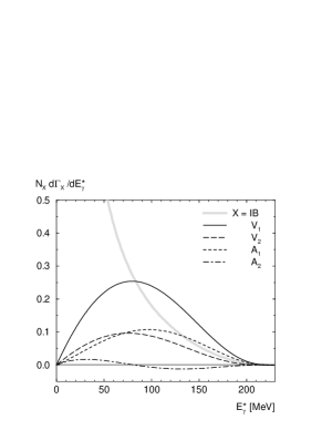
Figure 5: Photon energy distributions from inner bremsstrahlung as well as the various structure-dependent terms. The notation $d\Gamma_{X}/dE_{\gamma}^{*}$ for the various $X$ refers to (7.1). The normalization factors are $N_{V_{i},\,A_{i}}=200\,N_{\rm IB}=10^{3}M_{K}/\Gamma(K_{e3})$. We only cut on the electron-photon angle, $\theta_{e\gamma}^{\rm cut}=5^{\circ}$ ktev .

The relevant photon spectra are shown in Fig. 5. Note that the bremsstrahlung distribution is scaled down by a factor of 200 relative to the structure-dependent parts. We observe the expected fall-off of $d\Gamma_{\rm IB}/dE_{\gamma}^{*}\propto 1/E_{\gamma}^{*}$ as well as the linear rise of all structure-dependent spectra for small photon energies. As phase space bends them down to zero at maximum photon energy, all structure-dependent distributions show a maximum (a maximum and a minimum in the case of $A_{2}$), which for $V_{1}$, $V_{2}$ occurs around $E_{\gamma}^{*}=80$ MeV, for $A_{1}$ slightly higher, around $E_{\gamma}^{*}=100$ MeV. Although the $A_{2}$ spectrum has a form distinct from all others, its magnitude is far too small to be observable. In view of the chiral ${\cal O}(p^{4})$ prediction $A_{1}=0$, this means that no effects of the chiral anomaly are likely to be extracted from the photon energy spectrum.

The remaining three structure-dependent spectra are remarkably similar in shape, if not in height. If we assume that the experimental accuracy is not sufficient to observe the slightly shifted positions of the maxima in the three spectra, we have approximately

$$f(E_{\gamma}^{*})\;\doteq\;\frac{d\Gamma_{V_{1}}}{dE_{\gamma}^{*}}\;\approx\;2.6\times\frac{d\Gamma_{V_{2}}}{dE_{\gamma}^{*}}\;\approx\;2.4\times\frac{d\Gamma_{A_{1}}}{dE_{\gamma}^{*}}~{},$$ (7.2)

where we have taken the height of the peaks as the measure for the proportionality factors, irrespective of the exact energy where they occur. [In case that more accurate data is available, it would be straightforward to incorporate a more refined representation of the photon spectrum than the one proposed here.]

Equation (7.2) is the main result of our investigation of the photon spectrum:

1. To good approximation, the photon energy spectrum originating from the bremsstrahlung amplitude is distorted by one single function $f(E_{\gamma}^{*})$. The information on the SD terms is contained in the effective strength $\langle{X}\rangle$ that multiplies $f(E_{\gamma}^{*})$,

   $$\begin{split}\frac{d\Gamma}{dE_{\gamma}^{*}}&\,\approx\,\frac{d\Gamma_{\rm IB}}{dE_{\gamma}^{*}}+\langle{X}\rangle\;f(E_{\gamma}^{*})~{},\\ \langle{X}\rangle&\,=\,\langle{V_{1}}\rangle+0.4\,\langle{V_{2}}\rangle+0.4\,\langle{A_{1}}\rangle~{}.\end{split}$$ (7.3)

2. The three amplitudes $V_{1}$, $V_{2}$, $A_{1}$ differ mainly in terms of the weight with which they contribute to $\langle{X}\rangle\,.\,$ The latter can be calculated in ChPT,

   $$\langle{X}\rangle\,=\,\left\{\begin{array}[]{ll}-1.2&O(p^{4})\\[5.69054pt] -1.2\pm 0.4&O(p^{6})~{}.\end{array}\right.$$ (7.6)

   Note that the uncertainty in the contribution from the vector channel has only been roughly estimated here.

3. In order to measure $\langle{X}\rangle$, one may use the representation (7.3) for the spectrum, insert the explicit form of $f(E_{\gamma}^{*})$ and do a fit to the data with $\langle{X}\rangle$ as a free parameter. Alternatively, one may take any of the amplitudes $V_{1,2}$ or $A_{1}$, take it to be constant over phase space, and perform a fit to the bremsstrahlung spectrum. The result will be the same. However, it is clear that in this manner, one has not determined the chosen amplitude to perform the fit, but just the effective strength $\langle{X}\rangle$.

7.2 $E_{\gamma}^{*}$ distribution: experiment

We now discuss the result of the KTeV analysis ktev in light of the previous subsection. First, we note that in ktev , all SD parts were set to zero, except the amplitudes $C,D$, that were taken to be constant over phase space. This amounts to the procedure mentioned in point 3. above, except that two amplitudes have been retained in ktev , while one is sufficient to measure $\langle{X}\rangle$. Indeed, ktev finds a strongly eccentric error ellipse constraining the parameter space for these two structure-dependent terms. In order to compare the KTeV result with the above representation of $\langle{X}\rangle$, we translate the KTeV amplitudes into our conventions. We assume a linear form factor $f_{+}$, use the relations (6.6) and find that, with $A=B=0\,$,

$$V_{1}\,=\,C/M_{K}^{2}~{},~{}~{}V_{2}\,=\,4\dot{f}_{+}(0)~{},~{}~{}A_{1}\,=\,D/M_{K}^{2}~{}.$$ (7.7)

The $V_{i},A_{i}$ not listed are zero. In other words, the amplitudes (7.7) result in the same photon spectrum as the one generated by the amplitudes used in ktev . We therefore conclude that the effective strength $\langle{X}\rangle$ is given in this case by

$$\langle{X}\rangle\,=\,{C}+\tan{(23^{\circ})}{D}+1.5M_{K}^{2}\dot{f}_{+}(0)\,,\,$$ (7.8)

where we have dropped the bracket notation for $C,D$, because $\langle{C}\rangle=C$ for constant amplitudes, and the angle is introduced for easy comparison with ktev . The structure of (7.8) has been confirmed by the observation made in ktev that it is

$$C^{\prime}=\cos{(25.8^{\circ})}\bigl{[}C+\tan{(25.8^{\circ})}D\bigr{]}$$ (7.9)

which is best constrained by the data, with ktev

$$C^{\prime} = -2.5^{\,\,+1.5}_{\,\,-1.0}(\text{stat})\pm 1.5(\text{syst})~{}.$$ (7.10)

This may be compared with the calculation in the framework of ChPT. Using (7.8) and (7.6), and neglecting the small difference in the angle, we find

$$C^{\prime}=-1.6\pm 0.4\qquad{\mbox{\small{[ChPT]}}}\,,\,$$ (7.11)

which agrees with (7.10) rather well.

While an interpretation of the KTeV result (7.10) as a measurement of the effective coupling is sound, it does not allow one to draw conclusions about the size of the SD terms themselves because, as we have shown in the previous section, $C$ and $D$ are not observable amplitudes as long as the amplitude $V_{3}$ is not negligible. In addition, the assumption $A=B=0$ made in the analysis of ktev , on the basis of the soft kaon approximation, is incorrect and invalidates such an interpretation of $C^{\prime}$ even for a negligible $V_{3}$. Chiral perturbation theory may be used to illustrate this point: we consider the amplitudes at order $p^{4}$ and disregard the structure function $V_{3}$ altogether, then from (6.6), we find

$$\begin{split}\langle{X}\rangle&\,=\,\underbrace{{1.4\,\langle{A}\rangle}}_{-1.9}+\underbrace{{0.4\,\langle{B}\rangle}}_{+0.1}+\underbrace{{\langle{C}\rangle}}_{+0.1}+\underbrace{{0.4\,\langle{D}\rangle}}_{-0.1}+\underbrace{{1.5\,M_{K}^{2}\,\dot{f}_{+}(0)}}_{+0.6}\\ &\,=\,-1.2~{},~{}\end{split}$$ (7.12)

where we have again used the phase space average for the structure functions, because they are not constant in this case. Equation (7.12) shows that the main contribution to the effective strength $\langle{X}\rangle$ is due to the amplitude $A$, while ${C}$ plays a minor role, and the contribution from $D$ is canceled by the one from $B$. Therefore, the approximation of setting $A$ and $B$ to zero is not valid and, consequently, $\langle{X}\rangle$ is not dominated by $\langle{C}\rangle+0.4\langle{D}\rangle$, and should not be taken as a measure of this combination of amplitudes.

7.3 Systematic errors

We now discuss one potential source for systematic errors in this procedure of determining the effective strength $\langle{X}\rangle$ and start with the observation that the analysis obviously requires a rather precise knowledge of $d\Gamma_{\rm IB}/dE_{\gamma}^{*}$. As we consider unnormalized spectra, we are insensitive to overall coupling constants and $f_{+}(0)$, but we should investigate whether a shift in the $K_{e3}$ form factor parameters $\lambda_{+}$, $\lambda^{\prime\prime}_{+}$ can simulate a contribution to the spectrum similar to the structure-dependent effects. For this purpose, we expand a general bremsstrahlung spectrum with arbitrary form factor around our choice for these parameters,

$$\frac{d\Gamma_{\rm IB}}{dE_{\gamma}^{*}}\,=\,\frac{d\Gamma_{\rm IB}}{dE_{\gamma}^{*}}\Biggr{|}_{\!\!\begin{array}[]{l}\scriptstyle\bar{\lambda}_{+}=1\\[-2.84526pt] \scriptstyle\bar{\lambda}^{\prime\prime}_{+}=0\end{array}}\!+\,\bigl{(}\bar{\lambda}_{+}-1\bigr{)}\,\frac{d\Gamma_{\bar{\lambda}_{+}}}{dE_{\gamma}^{*}}\,+\,\bar{\lambda}^{\prime\prime}_{+}\,\frac{d\Gamma_{\bar{\lambda}^{\prime\prime}_{+}}}{dE_{\gamma}^{*}}\,+\,\ldots~{}.$$ (7.13)

The two spectra ${d\Gamma_{\bar{\lambda}_{+}}}/{dE_{\gamma}^{*}}$ and ${d\Gamma_{\bar{\lambda}^{\prime\prime}_{+}}}/{dE_{\gamma}^{*}}$ are displayed in Fig. 6 with a solid and a dashed line, respectively.

Figure 6: Photon energy distributions from inner bremsstrahlung, proportional to $(\bar{\lambda}_{+}-1)$ and $\bar{\lambda}^{\prime\prime}_{+}$, as well as a fine-tuned difference between the two. The normalization factors are given by $N_{\Delta\lambda}=100\,N_{\bar{\lambda}_{+}}=10\,N_{\bar{\lambda}^{\prime\prime}_{+}}=10^{3}M_{K}/\Gamma(K_{e3})$. We cut on the electron-photon angle with $\theta_{e\gamma}^{\rm cut}=5^{\circ}$ ktev .

We observe that they are rather sizeable, but very similar in shape to the overall IB spectrum. Only a fine-tuned cancellation of both can lead to a peak-like structure, which we find for

$$\alpha\,\doteq\,\frac{1-\bar{\lambda}_{+}}{\bar{\lambda}^{\prime\prime}_{+}}\,=\,0.080\pm 0.005~{}.$$ (7.14)

Stated differently, $\alpha$ has to be within this narrow range in order for the combination

$$\frac{d\Gamma_{\Delta\lambda}}{dE_{\gamma}^{*}}\;\,=\,\;\frac{d\Gamma_{\bar{\lambda}^{\prime\prime}_{+}}}{dE_{\gamma}^{*}}-\alpha\,\frac{d\Gamma_{\bar{\lambda}_{+}}}{dE_{\gamma}^{*}}$$ (7.15)

to have a maximum. This means that, for example, a simultaneous reduction of $\lambda_{+}$ by 8% as compared to the central input value and the introduction of a quadratic term in the form factor with $\lambda^{\prime\prime}_{+}=(\lambda_{+}^{c})^{2}$ (as suggested by $K^{*}$ pole saturation) mimics a structure-dependent contribution with a peak at roughly similar energies as $f(E_{\gamma}^{*})$.

The distribution (7.15) is displayed in Fig. 6 as a grey band at $\alpha=0.08$. Note that the strength of the peak is not big: for the chosen combination, it is about 10% of the dominant spectrum $\langle{V_{1}}\rangle d\Gamma_{V_{1}}/dE_{\gamma}^{*}$. To illustrate potential effects of this “background”, we compare these findings to the latest KTeV form factor measurements ktevlambda , $\bar{\lambda}_{+}=0.70\pm 0.06$, $\bar{\lambda}^{\prime\prime}_{+}=1.85\pm 0.40$. Taking into account the correlation ktevlambda between $\bar{\lambda}_{+}$ and $\bar{\lambda}^{\prime\prime}_{+}$, we find that they lead to $\alpha=0.16\pm 0.01$, and we conclude the following:

1. Although these values for $\bar{\lambda}_{+},\,\bar{\lambda}^{\prime\prime}_{+}$ are very different from our assumed central ones, they do not lead to a peak-like structure.

2. Even in the worst possible case with $\alpha\approx 0.08$ and $\bar{\lambda}^{\prime\prime}_{+}\approx 2$, the value for $\langle{X}\rangle$ based on the assumptions $\bar{\lambda}_{+}=1,\,\bar{\lambda}^{\prime\prime}_{+}=0$ is less negative than the true one. In other words, the modulus of $\langle{X}\rangle$ would be even bigger in the real world, by (20-25)%.

A more detailed analysis of this background phenomenon ought to be performed on real data.

7.4 Other distributions

We have emphasized that the study of the photon energy spectrum, at least with the currently achievable statistics, seems to give access to only one specific linear combination of structure-dependent terms, which is most sensitive to $V_{1}$. Ideally one would find alternative distributions that are more sensitive to the other terms $V_{2}$, $A_{1}$, $A_{2}$ in order to achieve a complete decomposition into the four (main) structure functions. The strategy for studying the various possible differential rates is to find those structure-dependent contributions that differ in shape from inner bremsstrahlung and, in contrast to $d\Gamma/dE_{\gamma}^{*}$, from each other. We have studied differential rates with respect to the other four independent variables $E_{\pi}^{*}$, ${E_{e}^{*}}$, $x$, $W^{2}$, but also to related variables $s$, $t$, $u$, $\cos\theta_{e\gamma}^{*}$, $\cos\theta_{\pi\gamma}^{*}$. Where applicable, we have used the cuts $E_{\gamma}^{\rm cut}=25$ MeV, $\theta_{e\gamma}^{\rm cut}=5^{\circ}$ in analogy to the procedure in ktev .

One general feature can already be seen from the $d\Gamma/dE_{\gamma}^{*}$ plots and appears in almost all distributions: the relative importance of $V_{1}$, $V_{2}$, $A_{1}$, $A_{2}$ is the same in most cases, as the integral over a differential rate has to be the same, no matter what kinematical variable is studied. Therefore distributions tend to be most sensitive to $V_{1}$, followed by $V_{2}$ and $A_{1}$ at roughly equal strength. The exception to this rule is $A_{2}$ that shows a sign change in most distributions, but again in most cases it is suppressed with respect to the other structure-dependent terms by at least one order of magnitude.

We shall only discuss those differential rates in some detail that seem to have interesting features. The distributions in $W^{2}$, $\cos\theta_{\pi\gamma}^{*}$ seem to offer no promising possibilities to extract information on any of the structure-dependent terms as their distributions are too similar to the dominant bremsstrahlung one, while those in ${E_{e}^{*}}$, $x$, or $s$ show $A_{2}$ curves that have interesting shapes (usually with an additional zero), but are probably far too much suppressed.

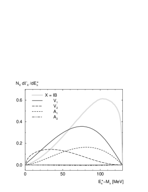
Figure 7: Pion energy distributions from inner bremsstrahlung as well as the various structure-dependent terms. The notation $d\Gamma_{X}/dE_{\pi}^{*}$ is chosen in analogy to (7.1). The normalization factors are $N_{V_{i},\,A_{i}}=200\,N_{\rm IB}=10^{3}M_{K}/\Gamma(K_{e3})$. The cuts $E_{\gamma}^{\rm cut}=25$ MeV, $\theta_{e\gamma}^{\rm cut}=5^{\circ}$ were applied.

More promising seem to be the partial rates $d\Gamma/dE_{\pi}^{*}$ that are displayed in Fig. 7. There is no divergent behavior visible in these distributions, all of them vanish at minimum and maximum pion energies, and the partial rates for bremsstrahlung as well as for $V_{1}$, $V_{2}$, and $A_{1}$ have one peak in the spectrum ($A_{2}$ is nearly completely suppressed here). We observe that the bremsstrahlung distribution is peaked at high pion energies (for $E_{\pi}^{*}-M_{\pi}\approx 100$ MeV), and so are the $V_{1}$ and $A_{1}$ partial rates, even though their respective peaks occur a bit lower. Distinct from all these is, however, the $V_{2}$ contribution to the pion energy distribution that is peaked at small pion energies. Although the overall sensitivity is again by roughly a factor of 3 smaller than that for $V_{1}$, this partial rate might be a window to access information on the structure function $V_{2}$.

We remark, though, that this extraction might again be obscured by uncertainties in the form factor $f_{+}$: the distributions $d\Gamma_{\bar{\lambda}_{+}}/dE_{\pi}^{*}$ and $d\Gamma_{\bar{\lambda}^{\prime\prime}_{+}}/dE_{\pi}^{*}$, defined in complete analogy to (7.13), also turn out to be peaked for lower pion energies than the total bremsstrahlung distribution. Of course this problem can be remedied by more precise form factor data as provided e.g. in ktevlambda ; Lai . A more detailed study should be performed with actual experimental data.

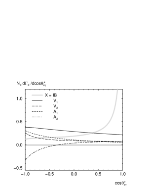
Figure 8: Distributions with respect to $\cos\theta_{e\gamma}^{*}$ from inner bremsstrahlung as well as the various structure-dependent terms. The notation $d\Gamma_{X}/d\cos\theta_{e\gamma}^{*}$ is chosen in analogy to (7.1). The normalization factors are $N_{V_{i},\,A_{i}}=200\,N_{\rm IB}=10^{4}/\Gamma(K_{e3})$. The photon energy cut $E_{\gamma}^{\rm cut}=25$ MeV was applied.

There is special interest in finding a partial rate with a more pronounced contribution from $A_{2}$ for the following reason: as discussed in Subsect. 6.1, this is the only non-vanishing contribution of the WZW-anomaly term, while $A_{1}$ vanishes at ${\cal O}(p^{4})$. We have commented before on the sign change in the $A_{2}$ distributions that often leads to cancellations. Fig. 8 shows a partial rate in which $A_{2}$ is relatively prominent: its contribution becomes relatively strong in $d\Gamma/d\cos\theta_{e\gamma}^{*}$ in backward direction. The slope of the total structure-dependent distribution in backward direction, which can be thought of as the second derivative with respect to $\cos\theta_{e\gamma}^{*}$ at $\cos\theta_{e\gamma}^{*}=-1$, is potentially dominated by $A_{2}$. It seems therefore that if effects of the chiral anomaly should be visible at all, it might be accessible in the distribution with respect to the electron-photon angle, in backward direction.

To conclude this section, we emphasize that this study of possible additional partial rates is by no means meant to be exhaustive. In particular, certain effects may only be visible in double differential rates etc. We defer any such more extensive study until experiments give hints about the statistical feasibility of these various suggestions.

8 Conclusions and outlook

In this paper, we have analyzed various aspects of $K_{e3\gamma}$ decays.

1. In the absence of radiative corrections, the decay amplitude may be decomposed into an inner brems- strahlung part (IB) and a structure-dependent part (SD). Our construction of the bremsstrahlung amplitude guarantees that the SD part is regular in the Mandelstam plane, aside from the branch points required by unitarity. Structure-dependent contributions can be parametrized in terms of eight structure functions $V_{i}\,,\,A_{i}\,,\,i=1,4$.

2. We evaluate the expression for the width with massless spinors. In other words, the electron mass is set to zero in the numerator of the relevant terms. In this approximation, the contribution from the IB part can be written entirely in terms of the $K_{e3}$ form factor $f_{+}$. Furthermore, the structure functions $V_{3}$ and $A_{3}$ cancel out.

3. If this IB–SD separation is applied to the chiral ${\cal O}(p^{4})$ representation of the $K_{e3\gamma}^{0}$ decay amplitude provided in BEG , one obtains leading-order chiral predictions for the structure functions (they vanish at order $p^{2}$). The axial terms are constant and given in terms of the WZW anomaly, while the vector terms receive contributions both from loop graphs and the low-energy constants ${L}_{9}^{r}$ and ${L}_{10}^{r}$ of the chiral Lagrangian at order $p^{4}$ GL . At this order, all cuts in the loop functions lie far outside the physical region, such that also the vector terms can be approximated to good accuracy by constants.

4. In order to obtain control of higher order corrections, we have analyzed ${\cal O}(p^{6})$ contributions to the structure-dependent terms. We have performed a complete calculation for the axial terms. For the vector ones, we have determined the $L_{i}\times L_{j}$ contributions at order $p^{6}$, and provided a very rough estimate of the remaining diagrams.

   At this order, cuts appear in the physical region, both in the axial and in the vector structure functions. The corresponding imaginary parts generate $T-$odd contributions in some of the decay distributions. On the other hand, in the cases considered in this work, they drop out.

   The effect of the cuts on the real parts is diminished by the fact that they appear as $P$-wave rescattering (axial) or only in a tiny corner of phase space (vector). Dominant uncertainties arise from $M_{K}^{2}$ corrections, generated by counterterms at ${\cal O}(p^{6})$.

5. The most precise and stable theoretical prediction can be given for the ratio $R$ of the radiative $K_{e3}$ decay width relative to the non-radiative one. This ratio turns out to be very insensitive to the details of the form factor $f_{+}$, such that the purely hadronic result is very precise. Structure-dependent terms yield only a 1% correction to the bremsstrahlung, such that even a sizeable uncertainty in the former affects the precision of the total value only at the few permille level. Our prediction for $E_{\gamma}^{\rm cut}=30\,$MeV, $\theta_{e\gamma}^{\rm cut}=20^{\circ}$,

   $$R=(0.96\pm 0.01)\times 10^{-2}~{},$$ (8.1)

   deviates from the KTeV results ktev_04 ; ktev , but agrees well with the recent measurement of the NA48 Collaboration na48 , see Table 1.

6. We have investigated the possibility to measure SD terms. We find that the bremsstrahlung spectrum is modified by the SD terms essentially by one single function $f(E_{\gamma}^{*})$, and that the different structure functions contribute with different strength to the effective coupling multiplying $f(E_{\gamma}^{*})$. The KTeV analysis ktev confirms this observation. In their language, the effective coupling is obtained from the combination

   $$C^{\prime}=\cos{(25.8^{\circ})}C+\sin{(25.8^{\circ})}D$$ (8.2)

   of amplitudes $C,D$, with ktev

   $$C^{\prime} = -2.5^{\,\,+1.5}_{\,\,-1.0}(\text{stat})\pm 1.5(\text{syst})~{}.$$ (8.3)

   The calculation in the framework of ChPT gives

   $$C^{\prime}=-1.6\pm 0.4\qquad{\mbox{\small{[ChPT]}}}\,.\,$$ (8.4)

   We have shown why the result (8.3) should not be interpreted as a measurement of the amplitudes $C,D$, but rather as a measurement of the effective coupling of the SD terms to $f(E_{\gamma}^{*})$.

7. We have discussed alternative distributions over phase space in a qualitative manner. In order to distinguish the vector functions $V_{1}$, $V_{2}$, the distribution in pion energies might be used. Effects of the chiral anomaly are highly suppressed in most distributions. It might at best be accessible in the differential rate with respect to the electron-photon angle in backward direction.

Most extensions of this work will depend on the further interplay between experimental accuracy and theoretical desirability: for example, a complete calculation of the radiative corrections would be desirable. We have refrained here from comparing to the latest KTeV results on $R$ without cuts on the photon–electron angle ktev_04 , as this also would necessitate special care concerning radiative corrections; this will be considered elsewhere. As indicated in the above, a more detailed study of how to disentangle the various structure-dependent terms would be possible once the extraction of such terms from experiment becomes feasible.

The most imminent extension of this work, however, is to provide predictions also for the other $K_{l3\gamma}$ channels. An analogous study of the charged channel $K_{e3\gamma}^{+}$ is most straightforward and will be performed in due course. The muon channels might in principle lend easier access to structure-dependent contributions. The KTeV experimental determinations of the ratio $R$ for $K_{L}\to\pi^{\pm}\mu^{\mp}\nu_{\mu}\gamma$ ktev_04 , with improved uncertainty with respect to the previous NA48 results bender , can already be considered as an interesting starting point for a more comprehensive study of radiative $K_{\mu 3}$ decays.

Acknowledgements

We thank Fabrizio Scuri for collaboration in an early stage of this work. We enjoyed informative discussions and/or e-mail exchanges with Douglas R. Bergman, Yury Bystritsky, Eduard Kuraev, Rick Kessler, Leandar Litov, Helmut Neufeld, Massimo Passera, Hannes Pichl, Martin Schmid, Stoyan Stoynev, and Rainer Wanke. In particular, we thank Alberto Sirlin for correspondence concerning the KLN theorem, and Konrad Kleinknecht for useful comments on the manuscript. This work was supported by the Swiss National Science Foundation, by RTN, BBW-Contract No. 01.0357, and EC-Contract HPRN–CT2002–00311 (EURIDICE). NP was partially supported by funds of MIUR (Italian Ministry of University and Research) and of the Trieste University.

Appendix A Notation

We denote the charged pion and neutral kaon masses with $M_{\pi}$ and $M_{K}$, respectively. In numerical evaluations, we use

$$M_{K} \,=\,497.67~{}\text{MeV}~{},~{}~{}M_{\pi}\,=\,139.57~{}\text{MeV}~{},~{}~{}$$ (A.1)

$$m_{e} \,=\,0.511~{}\text{MeV}~{},~{}~{}F_{\pi}\,=\,92.4~{}\text{MeV}~{},~{}~{}F_{K}\,=\,1.22\,F_{\pi}~{}.$$

The $K_{e3}$ form factor is parametrized by

$$f_{+}(t)\,=\,f_{+}(0)\left[1+\lambda_{+}\frac{t}{M_{\pi}^{2}}+\lambda^{\prime\prime}_{+}\frac{t^{2}}{M_{\pi}^{4}}+\cdots\right]~{}.$$ (A.2)

As explained in the main text, the precise values of $f_{+}(0)$ and $\lambda_{+}$ do not matter in the present context. For numerical evaluations, we use the parameter-free one-loop result leutroos

$$f_{+}(0)\,=\,0.977~{},$$ (A.3)

and a central value $\lambda_{+}^{c}=0.0294$. For the low-energy constants we take

$$L_{9}^{r}(M_{\rho})\,=\,6.3\times 10^{-3}~{},~{}~{}L_{10}^{r}(M_{\rho})=-4.9\times 10^{-3}~{}.$$ (A.4)

$L_{9}^{r}$ was chosen such that the chiral one-loop representation for $\lambda_{+}$ reproduces $\lambda_{+}^{c}=0.0294$. The sum $L_{9}^{r}+L_{10}^{r}$ is then fixed from $\pi_{e2\gamma}$ decays. We express the low-energy constants in the following, scale-independent form BEG :

$$\begin{split}\bar{L}_{9}&\,=\,L^{r}_{9}(\mu)-\frac{1}{512\pi^{2}}\log\frac{M_{\pi}^{2}M_{K}^{4}M_{\eta}^{2}}{\mu^{8}}~{},\\ \bar{L}_{10}&\,=\,L^{r}_{10}(\mu)+\frac{1}{512\pi^{2}}\log\frac{M_{\pi}^{2}M_{K}^{4}M_{\eta}^{2}}{\mu^{8}}~{}.\end{split}$$ (A.5)

Again, the precise values of $L^{r}_{9}$ and $L^{r}_{10}$ do not matter.

Appendix B Traces and decay widths

Here, we give the explicit expression for the sum over spins in $|T|^{2}$ in the limit where the relevant traces are evaluated at $m_{e}=0$, and comment on the relation between $K_{e3\gamma}$ and $K_{e3\gamma}^{0}$ decays in the presence of $T$-odd terms.

B.1 Traces

We write

$$\begin{split}N^{-1}\sum_{\rm spins}|T|^{2}\ &\,=\,a_{1}f_{+}(t)^{2}+a_{2}f_{+}(t)\delta f_{+}+a_{3}\delta f_{+}^{\,2}\\ &\,+\,\sum_{i=1}^{4}\Bigl{[}\bigl{(}b_{i}\,\text{Re}V_{i}+b^{5}_{i}\,\text{Re}A_{i}\bigr{)}f_{+}(t)\\ &\hskip 28.45274pt+\bigl{(}c_{i}\,\text{Re}V_{i}+c^{5}_{i}\,\text{Re}A_{i}\bigr{)}\delta f_{+}\Bigr{]}\\ &\,+\,\xi\,\sum_{i=1}^{4}\Bigl{[}\bigl{(}d_{i}\,\text{Im}V_{i}+d^{5}_{i}\,\text{Im}A_{i}\bigr{)}f_{+}(t)\\ &\hskip 28.45274pt+\bigl{(}e_{i}\,\text{Im}V_{i}+e^{5}_{i}\,\text{Im}A_{i}\bigr{)}\delta f_{+}\Bigr{]}\\ &\,+\,{\cal O}(V_{i}^{2},A_{i}^{2},V_{i}A_{i})\,,\,\end{split}$$ (B.1)

with

$$\begin{split}\xi&\,=\,M_{K}^{-3}{\bf q}\cdot({\bf p^{\prime}}\times{\bf p_{e}})~{},\\[5.69054pt] \delta f_{+}&\,=\,M_{K}^{2}(qW)^{-1}\left[f_{+}(t)-f_{+}(W^{2})\right]~{},\\[5.69054pt] N&={16\pi\alpha G_{F}^{2}|V_{us}|^{2}M_{K}^{2}}~{}.\end{split}$$ (B.2)

With this convention for $N$, the right hand side in (B.1) is dimensionless. In the limit $m_{e}=0$, we immediately have

$$b_{3}\,=\,b_{3}^{5}\,=\,c_{3}\,=\,c_{3}^{5}\,=\,d_{3}\,=\,d_{3}^{5}\,=\,e_{3}\,=\,e_{3}^{5}\,=\,0~{}.$$ (B.3)

We use the abbreviations

$$\begin{array}[]{lllll}z\,pp^{\prime}=a\,,&z\,pq=b\,,&z\,pp_{e}=c\,,&z\,pp_{\nu}=d\,,\\[5.69054pt] z\,p^{\prime}q=e\,,&z\,p^{\prime}p_{e}=f\,,&z\,p^{\prime}p_{\nu}=g\,,&z\,qp_{e}=h\,,\\[5.69054pt] z\,qp_{\nu}=j\,,&z\,p_{e}p_{\nu}=k\,,&z\,pW=l\,,&z\,p^{\prime}W=m\,,\\[5.69054pt] z\,qW=n\,,&z\,M_{\pi}^{2}=r\,,&z\,=M_{K}^{-2}\,,&\end{array}$$ (B.4)

and decompose all the coefficients according to $a_{i}=\hat{a}_{i}\,\bar{a}_{i}$ etc., where the prefactors $\hat{a}_{i}\,,\;\hat{b}_{i}\,\ldots$ are collected in Table B.1.

Table B.1: Prefactors that multiply the $\bar{a}_{i}\,,\;\bar{b}_{i}$ etc.

$\hat{a}_{1}$	$4/(e^{2}\,h)$	$\hat{b}_{1}$	$4/(e\,h)$	$\hat{b}^{5}_{1}$	$4/h$
$\hat{a}_{2}$	$1/(e^{2}\,h)$	$\hat{b}_{2}$	$4/(e\,h)$	$\hat{b}^{5}_{2}$	$4/(e\,h)$
$\hat{a}_{3}$	$4/e^{2}$	$\hat{b}_{4}$	$1/(e\,h)$	$\hat{b}^{5}_{4}$	$2/h$
$\hat{c}_{1}$	$4/e$	$\hat{c}^{5}_{1}$	$1$	$\hat{d}_{1}$	$4/(e\,h)$
$\hat{c}_{2}$	$1/e$	$\hat{c}^{5}_{2}$	$4\,n/e$	$\hat{d}_{2}$	$4/(e\,h)$
$\hat{c}_{4}$	$1/e$	$\hat{c}^{5}_{4}$	$1$	$\hat{d}_{4}$	$2/(e\,h)$
$\hat{d}^{5}_{1}$	$1/h$	$\hat{e}_{1}$	$4/e$	$\hat{e}^{5}_{1}$	$1$
$\hat{d}^{5}_{2}$	$4/(e\,h)$	$\hat{e}_{2}$	$4/e$	$\hat{e}^{5}_{2}$	$4\,n/e$
$\hat{d}^{5}_{4}$	$2/h$	$\hat{e}_{4}$	$4\,n/e$	$\hat{e}^{5}_{4}$	$1$

We obtain the following expressions for the coefficients $\bar{a}_{i}$, $\bar{b}_{i}$ and so on:

$$\bar{a}_{1} = 2\,b\,d\,e\,(e+f)-e\,\bigl{[}h\,(2\,a\,d-g)+j\,(e+f)$$

$$+k\,(e+2\,f)\bigr{]}+h\,k\,r+2\,c\,d\,(e^{2}+2\,e\,f-h\,r)\,,\,$$

$$\bar{a}_{2} = 4\,e\,\bigl{\{}e\,k\,\bigl{[}2\,d\,(2\,c-h)+h-j\,(1+2\,c)-2\,k$$

$$+2\,b\,(d-h+k)\bigr{]}-2\,e\,h\,l\,(d-j)$$

$$+2\,h\,m\,\bigl{[}d\,h+c\,(j-2\,d)+k\,(1-b)\bigr{]}\bigr{\}}$$

$$-4\,n\,\bigl{\{}2\,b\,d\,e\,f+e\,h\,\bigl{[}2\,d\,(-a+e+f)+g\bigr{]}$$

$$-e\,f\,j-2\,e\,k\,(f+a\,h)+2\,h\,k\,r$$

$$+2\,c\,(2\,d\,e\,f+e\,g\,h-2\,d\,h\,r)\bigr{\}}\,,\,$$

$$\bar{a}_{3} = -2\,e^{2}\,k\,\bigl{[}2\,(c-h)\,(d-j)+k\,(2\,b-1)\bigr{]}$$

$$-2\,e\,n\,\bigl{\{}e\,k\,(c+d-h-j-l)$$

$$+m\,\bigl{[}d\,h+c\,(j-2\,d)+k\,(1-b)\bigr{]}\bigr{\}}$$

$$+n^{2}\,\bigl{[}2\,e\,(d\,f+c\,g-a\,k)+r\,(k-2\,c\,d)\bigr{]}\,,\,$$

$$\bar{b}_{1} = e\,\bigl{[}d\,h\,(e+2\,f)+g\,h\,(b+c)+j\,(c\,f-a\,h)$$

$$-k\,(b\,f+a\,h)\bigr{]}-h\,r\,(d\,h+c\,j-b\,k)\,,\,$$

$$\bar{b}_{2} = j\,(c\,e\,k-e\,h\,l-c\,h\,m)+b\,k\,\bigl{[}e\,(h-k)+h\,m\bigr{]}$$

$$+n\,h\,(c\,g-a\,k)+d\,h\,\bigl{[}e\,k-h\,m+n\,(e+f)\bigr{]}\,,\,$$

$$\bar{b}_{4} = 2\,e\,\bigl{\{}c\,e\,k\,(e-2\,g)+e\,\bigl{[}-b\,k\,(f+g)$$

$$+a\,k\,(j-h+2\,k)+l\,(g\,h+f\,j-e\,k)\bigr{]}$$

$$+c\,m\,(2\,g\,h-e\,j)+k\,m\,(b\,e-2\,a\,h)$$

$$+d\,(e+2\,f)\,(-e\,k+h\,m)\bigr{\}}$$

$$+2\,n\,\bigl{\{}-\bigl{[}e\,(c\,g\,(e-2\,f)-2\,b\,f\,g$$

$$+a\,(-e\,k+2\,f\,(j+k)))\bigr{]}+r\,\bigl{[}c\,(-2\,g\,h+e\,j)$$

$$+k\,(-b\,e+2\,a\,h)\bigr{]}+d\,(e+2\,f)\,(e\,f-h\,r)\bigr{\}}\,,\,$$

$$\bar{b}^{5}_{1} = h\,(d\,e+b\,g+c\,g)-j\,(c\,f+a\,h)+k\,(b\,f-a\,h)\,,\,$$

$$\bar{b}^{5}_{2} = c\,e\,k\,(j-h)-b\,k\,\bigl{[}h\,(e+f-g)+e\,k\bigr{]}$$

$$+h\,\bigl{[}a\,k\,(h-j)+l\,(-g\,h+e\,j+f\,j+e\,k)-d\,e\,n\bigr{]}\,,\,$$

$$\bar{b}^{5}_{4} = k\,\bigl{\{}-d\,e^{2}+a\,(e-2\,f)\,(j-h)$$

$$+b\,\bigl{[}2\,f\,(g-f)-e\,(g+f)\bigr{]}\bigr{\}}+k^{2}\,(-2\,r\,b+2\,a\,e)$$

$$+l\,\bigl{[}g\,h\,(e-2\,f)+(e+2\,f)\,(f\,j-e\,k)+2\,r\,h\,k\bigr{]}$$

$$+m\,(d\,e\,h+b\,e\,k+2\,b\,f\,k-2\,a\,h\,k)$$

$$+n\,\bigl{[}f\,(d\,e+2\,b\,g-2\,a\,j)-r\,(b\,k+d\,h)+a\,e\,k\bigr{]}$$

$$+c\,\bigl{\{}k\,(e^{2}-2\,r\,h+2\,r\,j)+m\,(2\,g\,h-2\,f\,j)$$

$$+r\,j\,n+e\,\bigl{[}2\,f\,k-j\,m-g\,(2\,k+n)\bigr{]}\bigr{\}}\,,\,$$

$$\bar{c}_{1} = e\,\bigl{\{}e\,k\,(d-h-j-l)+m\,(2\,h\,j+b\,k-d\,h)$$

$$+c\,(e\,k-j\,m)\bigr{\}}-e\,n\,\bigl{[}g\,(c+h)+f\,(d+j)-a\,k\bigr{]}$$

$$+n\,r\,(d\,h+c\,j-b\,k)\,,\,$$

$$\bar{c}_{2} = 8\,e\,k\,\bigl{[}2\,h\,j+b\,k-d\,h-c\,j\bigr{]}$$

$$+4\,n\,\bigl{\{}e\,k\,(c+d-2\,(h+j)-l)$$

$$+m\,(d\,h+c\,j-b\,k)\bigr{\}}-4\,n^{2}\,(d\,f+c\,g-a\,k)\,,\,$$

$$\bar{c}_{4} = 8\,e^{2}\,k\,(d\,f+c\,g-g\,h-f\,j-a\,k+e\,k)$$

$$+4\,e\,n\,\bigl{[}e\,k\,(f+g-2\,m)$$

$$+m\,(-2\,d\,f-2\,c\,g+g\,h+f\,j+2\,a\,k)\bigr{]}$$

$$+4\,n^{2}\,\bigl{[}r\,(d\,f+c\,g+k\,(e-a))-2\,e\,f\,g\bigr{]}\,,\,$$

$$\bar{c}^{5}_{1} = 4\,\bigl{[}b\,k\,(g-f)-e\,h\,k+a\,k\,(h-j)+e\,j\,k$$

$$-g\,h\,l+f\,j\,l-g\,h\,n+f\,j\,n\bigr{]}\,,\,$$

$$\bar{c}^{5}_{2} = b\,k\,(f-g)-k\,(a-2\,e)\,(h-j)+l\,(g\,h-f\,j)\,,\,$$

$$\bar{c}^{5}_{4} = 4\,n\,\bigl{[}e\,k\,(g-f)+r\,k\,(h-j)+m\,(f\,j-g\,h)\bigr{]}\,.\,$$

The coefficients for the $T$-odd terms are

$$\begin{array}[]{ll}\bar{d}_{1}=-e\,f+r\,h~{},&~{}\bar{d}_{2}=h\,(f+g+h+j)+e\,(h-k)~{},\\[5.12149pt] \lx@intercol\bar{d}_{4}=2\,e^{2}\,g+2\,e\,h\,(f+g)-r\,e\,(h+j)-2\,r\,h\,(h+j)~{},\hfil\lx@intercol\\[5.12149pt] \bar{d}^{5}_{1}=4\,f~{},&~{}\bar{d}^{5}_{2}=h\,(j-f+g-h)-e\,(h+k)~{},\\[5.12149pt] \lx@intercol\bar{d}^{5}_{4}=g\,(2\,e+4\,f)+2\,h\,(g-f)-r\,(h+j+2\,k)~{},\hfil\lx@intercol\end{array}$$ (B.6)

and

$$\begin{array}[]{ll}\bar{e}_{1}=-r\,n+e\,(f+g)~{},&~{}\bar{e}_{2}=2\,e\,k-n\,(f+g+h+j)~{},\\[5.12149pt] \lx@intercol\bar{e}_{4}=r\,(h+j)-e\,(f+g)~{},\hfil\lx@intercol\\[5.12149pt] \bar{e}^{5}_{1}=4\,(g-f)~{},&~{}\bar{e}^{5}_{2}=f-g+h-j~{},\\[5.12149pt] \lx@intercol\bar{e}^{5}_{4}=4\,n\,(f-g)~{}.\hfil\lx@intercol\end{array}$$ (B.7)

B.2 On the relation between $K_{L}$ and $K^{0}$ decays

Here we comment on the decay $K_{L}\rightarrow\pi^{\pm}e^{\mp}\nu_{e}\gamma$ and its relation to $K^{0}\rightarrow\pi^{-}e^{+}\nu_{e}\gamma$ in light of the contributions proportional to $\xi$ in (B.1). We neglect ${CP}$-violating contributions and write

$$|K_{L}\rangle\,=\,\frac{1}{\sqrt{2}}\left(|K^{0}\rangle-|\bar{K}^{0}\rangle\right)\,.\,$$ (B.8)

The width for $K_{L}\rightarrow\pi^{\pm}e^{\mp}\nu_{e}\gamma$ is proportional to

$$\int d_{\rm LIPS}\bigl{(}C_{1}+C_{2}\bigr{)}~{},$$ (B.9)

where

$$\begin{split}C_{1}&\,=\,\sum_{\rm spins}\bigl{|}T\bigl{(}K_{L}\to\pi^{-}e^{+}\nu_{e}\gamma\bigr{)}\bigr{|}^{2}~{},\\ C_{2}&\,=\,\sum_{\rm spins}\bigl{|}T\bigl{(}K_{L}\to\pi^{+}e^{-}\bar{\nu}_{e}\gamma\bigr{)}\bigr{|}^{2}~{}.\end{split}$$ (B.10)

In $C_{1}\,(C_{2})$, only the component $|K^{0}\rangle$ ($|\bar{K}^{0}\rangle$) contributes. We use $CP$ to transform the second term to the first one. Doing so, all three-momenta of the particles change sign. Therefore, terms proportional to $\xi$ drop out in the sum $C_{1}+C_{2}\,$, and the decay width for $K_{L}\rightarrow\pi^{\pm}e^{\mp}\nu_{e}\gamma$ agrees with the one for $K^{0}\rightarrow e^{+}\nu_{e}\pi^{-}\gamma\,$, because in this decay, $\xi$ drops out as well after integration over the momenta. These remarks remain true in the presence of the kinematical cuts considered in the main text, in connection with the ratio $R$. Therefore, up to terms quadratic in the structure-dependent terms, only the real parts of the amplitudes $V_{i},A_{i}$ occur in the width and in $R$. Finally, the decay width for $K^{0}\rightarrow\pi^{-}e^{+}\nu_{e}$ coincides with $\Gamma(K_{e3})$. This leads to the expression (5.5) for the ratio ${\cal R}$.

For $T$-odd terms in the context of $K^{+}_{e3\gamma}$ decays, see braguta .

Appendix C Invariant amplitudes for $K_{l3\gamma}^{0}$ at order $p^{4}$

In this appendix, we wish to give a simplified form of the $K_{l3\gamma}^{0}$ one-loop amplitudes that is nevertheless as accurate as the exact result (that can be found in BEG ) for all practical purposes. As the structure-dependent terms start to contribute at ${\cal O}(q)$, we intend to retain only terms of order linear in the photon momentum and neglect everything that is ${\cal O}(q^{2})$ or higher. In this approximation, all the structure functions $V_{1/2/3}$ can be written in terms of the conventional two-point function $\bar{J}(t)$ plus chiral logarithms and rational functions of the masses. As remarked before, $V_{4}=0$ at this order. We use the following definitions and conventions:

$$M_{1} \,=\,M_{K}~{},~{}~{}m_{1}\,=\,M_{\pi}~{},~{}~{}M_{2}\,=\,M_{\eta}~{},~{}~{}m_{2}\,=\,M_{K}~{},$$

$$\Sigma_{i} \,=\,M_{i}^{2}+m_{i}^{2}~{},~{}~{}\Delta_{i}\,=\,M_{i}^{2}-m_{i}^{2}~{},$$ (C.1)

the Källén function

$$\lambda_{i}(t) \,=\,\lambda(t,M_{i}^{2},m_{i}^{2})$$ (C.2)

$$\,=\,t^{2}+M_{i}^{4}+m_{i}^{4}-2\left(t\left(M_{i}^{2}+m_{i}^{2}\right)+M_{i}^{2}m_{i}^{2}\right)~{},$$

and the loop functions

$$\bar{J}_{1}(t) \,=\,\bar{J}_{K\pi}(t)~{},\quad\bar{J}_{2}(t)\,=\,\bar{J}_{\eta K}(t)~{},$$

$$\bar{J}_{ab}(t) \,=\,J_{ab}(t)-J_{ab}(0)~{},$$ (C.3)

$$J_{ab}(q^{2}) \,=\,\frac{1}{i}\int\frac{d^{d}l}{(2\pi)^{d}}\frac{1}{\bigl{(}M_{a}^{2}-l^{2}\bigr{)}\bigl{(}M_{b}^{2}-(l-q)^{2}\bigr{)}}~{}.$$

Our results can be written as follows:

$$V_{1} = -\frac{8}{F^{2}}\bar{L}_{9}$$

$$- \frac{1}{4F^{2}t}\sum_{i=1}^{2}\biggl{\{}\biggl{(}\frac{2\lambda_{i}(t)}{t}+3\Sigma_{i}+\left(M_{K}^{2}-M_{\pi}^{2}\right)\biggr{)}\bar{J}_{i}(t)$$

$$+\frac{t\Sigma_{i}-2M_{i}^{2}m_{i}^{2}}{16\pi^{2}\Delta_{i}}\log\frac{m_{i}^{2}}{M_{i}^{2}}+\frac{t-3\Sigma_{i}}{48\pi^{2}}\biggl{\}}+{\cal O}(q)~{},$$

$$V_{2} = \frac{4}{F^{2}}\left(\bar{L}_{9}+\bar{L}_{10}\right)$$

$$- \frac{1}{2F^{2}}\biggl{\{}\frac{M_{K}^{2}+M_{\pi}^{2}}{t}\bar{J}_{1}(t)-\frac{1}{16\pi^{2}}+\frac{4M_{K}^{2}M_{\pi}^{2}}{\lambda_{1}(t)}\times$$

$$\quad\times\biggl{(}\bar{J}_{1}(t)-\frac{1}{16\pi^{2}}-\frac{t-\left(M_{K}^{2}+M_{\pi}^{2}\right)}{32\pi^{2}\left(M_{K}^{2}-M_{\pi}^{2}\right)}\log\frac{M_{K}^{2}}{M_{\pi}^{2}}\biggr{)}\biggr{\}}$$

$$+ \frac{1}{2F^{2}t}\sum_{i=1}^{2}\biggl{\{}\frac{2M_{i}^{2}m_{i}^{2}}{\lambda_{i}(t)}\Bigl{(}2t+3\left(M_{K}^{2}-M_{\pi}^{2}\right)+\Delta_{i}\Bigr{)}\times$$

$$\qquad\times\Bigl{(}\bar{J}_{i}(t)-\frac{1}{16\pi^{2}}\Bigr{)}$$

$$+\biggl{(}3m_{i}^{2}+\frac{2m_{i}^{2}\Delta_{i}}{t}+\frac{3(M_{K}^{2}-M_{\pi}^{2})\Delta_{i}^{2}}{t^{2}}\biggr{)}\bar{J}_{i}(t)$$

$$+\frac{M_{i}^{2}m_{i}^{2}}{16\pi^{2}\Delta_{i}}\log\frac{m_{i}^{2}}{M_{i}^{2}}\biggl{[}3\left(1-\frac{M_{K}^{2}-M_{\pi}^{2}}{t}\right)+\frac{2t\Sigma_{i}}{\lambda_{i}(t)}$$

$$+\frac{3(M_{K}^{2}-M_{\pi}^{2})+\Delta_{i}}{2\lambda_{i}(t)}\times$$

$$\qquad\times\left(2(t-\Sigma_{i})-\Delta_{i}+\frac{3}{10}\left(M_{K}^{2}-M_{\pi}^{2}-\Delta_{i}\right)\right)\biggr{]}$$

$$-\frac{1}{16\pi^{2}}\biggl{(}t-m_{i}^{2}+\frac{M_{K}^{2}-M_{\pi}^{2}}{2t}\bigl{(}3\Sigma_{i}+t\bigr{)}\biggr{)}\biggr{\}}+{\cal O}(q)~{},$$

$$V_{3} = \frac{1}{2F^{2}t}\sum_{i=1}^{2}\biggl{\{}\frac{1}{t^{2}}\Bigl{(}\left(M_{K}^{2}-M_{\pi}^{2}\right)t+6\Delta_{i}^{2}\Bigr{)}\bar{J}_{i}(t)$$

$$-\frac{\bigl{(}3\Sigma_{i}+(M_{K}^{2}-M_{\pi}^{2})\bigr{)}(t-\Sigma_{i})-12M_{i}^{2}m_{i}^{2}}{2\lambda_{i}(t)}\times$$

$$\qquad\times\Bigl{(}\bar{J}_{i}(t)-\frac{1}{16\pi^{2}}\Bigr{)}$$

$$-\frac{M_{i}^{2}m_{i}^{2}}{16\pi^{2}t\Delta_{i}}\biggl{(}\frac{(M_{K}^{2}-M_{\pi}^{2})t+3\Delta_{i}^{2}}{\lambda_{i}(t)}+3\biggr{)}\log\frac{m_{i}^{2}}{M_{i}^{2}}$$

$$+\frac{t-6\Sigma_{i}}{32\pi^{2}t}\biggr{\}}+{\cal O}(q)~{}.$$

Note that this expansion necessarily upsets the analytic structure as the cuts in the variables $t$ and $W^{2}$ coincide in the limit of vanishing photon momentum. However, these cuts lie far outside the physical region (see discussion in Sect. 4.2). Furthermore, despite their appearance, all the functions above are regular and smooth at $t=0$ and $t=(M_{K}-M_{\pi})^{2}$. The results of the even further simplification by setting $t=0$ are displayed in the main text (4.3).

Appendix D Axial form factors at order $p^{6}$

Figure D.1: Diagrams that contribute to the anomalous amplitude $A_{\mu\nu}$ at order $p^{6}$ [in a), the contribution from $\pi,\eta$ intermediate states vanishes]. Charges of the mesons running in the loops are not indicated. The filled vertices denote a contribution from the anomalous Lagrangian at order $p^{4}$. External line insertions in the tree diagram of order $p^{4}$ are not displayed.

In this appendix, we give the explicit formulae for the next-to-leading order corrections to the axial form factors $A_{1}$, $A_{2}$, and $A_{4}$, as written out formally in (4.4)-(4.6). The necessary loop diagrams for this calculation are displayed in Fig. D.1. We find the following combinations of loop functions and counterterms:

$$S_{1}(s) \,=\,2H^{r}_{\pi\pi}(s)+\frac{16\pi^{2}}{3}\,C^{r}_{1s}\,s~{},$$ (D.1)

$$S_{2}(s) \,=\,\frac{16\pi^{2}}{3}\,C_{2s}\,s~{},$$ (D.2)

$$T_{1}(t) \,=\,H^{r}_{K\pi}(t)+H^{r}_{\eta K}(t)+\frac{16\pi^{2}}{3}\,C^{r}_{1t}\,t~{},$$ (D.3)

$$T_{2}(t) \,=\,T_{K\pi}^{r}(t)+T_{\eta K}^{r}(t)+\frac{16\pi^{2}}{3}\,C^{r}_{2t}\,t~{},$$ (D.4)

$$U_{1}(u) \,=\,-H^{r}_{K\pi}(u)-3H^{r}_{\eta K}(u)+\frac{16\pi^{2}}{3}\,C^{r}_{1u}\,u~{},$$ (D.5)

$$U_{2}(u) \,=\,2H^{r}_{K\pi}(u)+6H^{r}_{\eta K}(u)+\frac{16\pi^{2}}{3}\,C^{r}_{2u}\,u~{},$$ (D.6)

$$X_{1} \,=\,2\mu_{\pi}-\mu_{K}-\mu_{\eta}+\frac{16\pi^{2}}{3}\bigl{(}C^{r}_{1\pi}M_{\pi}^{2}+C^{r}_{1K}M_{K}^{2}\bigr{)}~{},$$ (D.7)

$$X_{2} \,=\,-\frac{31}{12}\mu_{\pi}+\frac{19}{6}\mu_{K}+\frac{3}{4}\mu_{\eta}$$

$$\hskip 14.22636pt+\frac{16\pi^{2}}{3}\bigl{(}C^{r}_{2\pi}M_{\pi}^{2}+C^{r}_{2K}M_{K}^{2}\bigr{)}~{}.~{}~{}$$ (D.8)

The loop function $H^{r}_{ab}(x)$ is defined as

$$\begin{split}H^{r}_{ab}(x)&=\frac{1}{12F^{2}}\biggl{\{}\frac{\lambda(x,M_{a}^{2},M_{b}^{2})}{x}\bar{J}_{ab}(x)+\frac{x-3\Sigma_{ab}}{24\pi^{2}}\\ &-\frac{x}{32\pi^{2}}\log\frac{M_{a}^{2}M_{b}^{2}}{\mu^{4}}-\frac{x\,\Sigma_{ab}-8M_{a}^{2}M_{b}^{2}}{32\pi^{2}\Delta_{ab}}\log\frac{M_{a}^{2}}{M_{b}^{2}}\biggr{\}}~{}.\end{split}$$ (D.9)

The other functions can also be written in relatively compact forms:

$$T_{K\pi}^{r}(t) \,=\,\frac{1}{24F^{2}}\biggl{\{}13t\biggl{[}\bar{J}_{K\pi}(t)$$

$$\hskip 28.45274pt-\frac{1}{32\pi^{2}}\Bigl{(}\log\frac{M_{K}^{2}M_{\pi}^{2}}{\mu^{4}}+\frac{\Sigma_{K\pi}}{\Delta_{K\pi}}\log\frac{M_{K}^{2}}{M_{\pi}^{2}}\Bigl{)}\biggr{]}$$

$$\hskip 14.22636pt-\biggl{[}2\Sigma_{K\pi}+16\Delta_{K\pi}$$

$$\hskip 28.45274pt-\Bigl{(}8\Sigma_{K\pi}-11\Delta_{K\pi}+\frac{8\Delta_{K\pi}^{2}}{t}\Bigr{)}\frac{\Delta_{K\pi}}{t}\biggr{]}\bar{J}_{K\pi}(t)$$

$$\hskip 14.22636pt+\frac{M_{K}^{2}M_{\pi}^{2}(2\Delta_{K\pi}+t)}{4\pi^{2}t\Delta_{K\pi}}\log\frac{M_{K}^{2}}{M_{\pi}^{2}}$$

$$\hskip 14.22636pt-\frac{(t-3\Sigma_{K\pi})(t-\Delta_{K\pi})}{12\pi^{2}t}\biggr{\}}~{},$$ (D.10)

$$T_{\eta K}^{r}(t) \,=\,\frac{1}{24F^{2}}\biggl{\{}t\biggl{[}\bar{J}_{\eta K}(t)$$

$$\hskip 28.45274pt-\frac{1}{32\pi^{2}}\Bigl{(}\log\frac{M_{\eta}^{2}M_{K}^{2}}{\mu^{4}}+\frac{\Sigma_{\eta K}}{\Delta_{\eta K}}\log\frac{M_{\eta}^{2}}{M_{K}^{2}}\Bigl{)}\biggr{]}$$

$$\hskip 14.22636pt+\biggl{[}2\Sigma_{\eta K}+8\Delta_{\eta K}$$

$$\hskip 28.45274pt-\Bigl{(}\frac{8}{3}\Sigma_{\eta K}+9\Delta_{\eta K}-\frac{8\Delta_{\eta K}^{2}}{t}\Bigr{)}\frac{\Delta_{K\pi}}{t}\biggr{]}\bar{J}_{\eta K}(t)$$

$$\hskip 14.22636pt+\frac{M_{\eta}^{2}M_{K}^{2}(2\Delta_{K\pi}-t)}{4\pi^{2}t\Delta_{\eta K}}\log\frac{M_{\eta}^{2}}{M_{K}^{2}}$$

$$\hskip 14.22636pt-\frac{(t-3\Sigma_{\eta K})(t-\Delta_{K\pi})}{12\pi^{2}t}\biggr{\}}~{},$$ (D.11)

$$\mu_{a} \,=\,\frac{M_{a}^{2}}{32\pi^{2}F^{2}}\log\frac{M_{a}^{2}}{\mu^{2}}~{},$$ (D.12)

where we have used $\Sigma_{ab}=M_{a}^{2}+M_{b}^{2}$, $\Delta_{ab}=M_{a}^{2}-M_{b}^{2}$, and the two point function $\bar{J}_{ab}(x)$ as defined in (C.3). The combinations of low-energy constants occurring in (4.4)–(4.6) and (D.1)–(D.8) are given in Table D.1 according to the numbering in p6anom .

Table D.1: The coefficients from (D.1)–(D.8) in terms of the renormalized low-energy constants $C_{i}^{Wr}$. For example, $C_{1s}^{r}=4C_{13}^{Wr}-10C_{14}^{Wr}+\ldots$. Constants without superscript $r$ are scale independent.

$${\begin{array}[]{lrrrrrrrrrrr}\hline\cr&C_{1s}^{r}&C_{1t}^{r}&C_{1u}^{r}&C_{1\pi}^{r}&C_{1K}^{r}&C_{2s}&C_{2t}^{r}&C_{2u}^{r}&C_{2\pi}^{r}&C_{2K}^{r}&C_{4A}\\ \hline\cr C_{2}^{Wr}&0&0&0&24&-24&0&0&0&-48&48&0\\ C_{4}^{Wr}&0&0&0&8&-16&0&0&0&-16&0&0\\ C_{5}^{Wr}&0&0&0&-8&16&0&0&0&16&0&0\\ C_{7}^{W}&0&0&0&0&0&0&0&0&-16&-32&0\\ C_{9}^{W}&0&0&0&0&0&0&0&0&0&48&0\\ C_{11}^{Wr}&0&0&0&0&0&0&0&0&0&-48&0\\ C_{13}^{Wr}&4&4&4&-10&2&-8&-10&0&22&10&-16\\ C_{14}^{Wr}&-10&-10&-4&12&18&20&16&0&-20&-16&48\\ C_{15}^{Wr}&8&8&8&-12&-12&-16&-20&0&28&20&-32\\ C_{19}^{Wr}&2&2&2&-2&-2&-4&-2&0&2&2&0\\ C_{20}^{Wr}&-2&-2&-8&8&2&4&8&0&-20&-8&16\\ C_{21}^{Wr}&4&4&4&-4&-4&-8&-4&0&4&4&0\\ C_{22}^{Wr}&-1&-1&-4&4&1&6&4&8&-10&-4&8\\ C_{23}^{W}&9&9&6&-6&-9&-18&-12&-12&6&12&8\\ \hline\cr\end{array}}$$ (D.28)

Appendix E Inner bremsstrahlung in $K_{l3\gamma}^{0}$ decays

In this appendix we discuss the separation of the hadronic tensor $V_{\mu\nu}$ into an IB and a SD part. To be specific, we imagine a calculation in the framework of ChPT to all orders and discuss the decomposition there.

Figure E.1: Diagrams for $V_{\mu\nu}$, evaluated in the framework of ChPT. The hatched blobs denote one-particle irreducible graphs.

The relevant diagrams can be grouped in two classes, displayed in Fig. E.1. The hatched blobs denote one-particle irreducible contributions. The diagram b) generates a pole in the variable $s=(p^{\prime}+q)^{2}$, at $s=M_{\pi}^{2}$, corresponding to the intermediate pion state. We isolate the contribution of this pole by writing

$$V_{\mu\nu}\,=\,\tilde{V}_{\mu\nu}+\frac{p^{\prime}_{\mu}}{p^{\prime}q}\,\left[2p_{\nu}f_{+}(W^{2})-W_{\nu}f_{2}(W^{2})\right]~{},$$ (E.1)

where $W=p-p^{\prime}-q$. In the following, we assume that this is the only singular part at $q=0$ in the tensor $V_{\mu\nu}$, or, in other words, that $\tilde{V}_{\mu\nu}$ is regular at $q=0$. This is the only assumption in the derivation of the final expression for the IB term. We have checked that it is true at one-loop order in ChPT, see below, and we see no reason why it should not be correct to any order, and thus true in QCD. Next, we write this regular part as

$$\begin{split}\tilde{V}_{\mu\nu}&\,=\,v_{0}\,g_{\mu\nu}+v_{1}\,p^{\prime}_{\mu}q_{\nu}+v_{2}\,W_{\mu}q_{\nu}+v_{3}\,p^{\prime}_{\mu}W_{\nu}\\ &\hskip 12.80365pt+v_{4}\,p^{\prime}_{\mu}p^{\prime}_{\nu}+v_{5}\,W_{\mu}p^{\prime}_{\nu}+v_{6}\,W_{\mu}W_{\nu}~{}.\end{split}$$ (E.2)

The Ward identity (3.6) generates three conditions on $\tilde{V}_{\mu\nu}$,

$$\begin{split}v_{0}+v_{1}\,p^{\prime}q+v_{2}\,qW&\,=\,2\triangle f_{+}-f_{2}~{},\\ v_{3}\,p^{\prime}q+v_{6}\,qW&\,=\,2\triangle f_{+}-\triangle f_{2}~{},\\ v_{4}\,p^{\prime}q+v_{5}\,qW&\,=\,2\triangle f_{+}~{},\end{split}$$ (E.3)

with

$$\triangle f_{i}\,=\,f_{i}(t)-f_{i}(W^{2})~{}.$$ (E.4)

The first equation can be solved for $v_{0}$. Furthermore, we set

$$v_{5}\,=\,\frac{2\triangle f_{+}}{qW}+\tilde{v}_{5}~{},~{}~{}v_{6}\,=\,\frac{2\triangle f_{+}-\triangle f_{2}}{qW}+\tilde{v}_{6}~{}.$$ (E.5)

and are left with

$$\begin{split}v_{4}\,p^{\prime}q+\tilde{v}_{5}\,qW\,=\,0~{},\\ v_{3}\,p^{\prime}q+\tilde{v}_{6}\,qW\,=\,0~{}.\end{split}$$ (E.6)

At this stage, we use the fact that the Lorentz invariant amplitudes $v_{i}$ are defined for any value of the kinematic variables $p^{\prime}q,qW$, and that the amplitudes are assumed to be non-singular at $p^{\prime}q=0$. It then follows that $\tilde{v}_{5,6}$ are proportional to $p^{\prime}q$,

$$\tilde{v}_{5,6}\,=\,-p^{\prime}q\,\tilde{v}_{4,3}~{}.$$ (E.7)

where the sign and the numbering is chosen for convenience. Finally, we obtain

$$v_{3,4}\,=\,qW\,\tilde{v}_{3,4}~{}.$$ (E.8)

Collecting the results, we find that $V_{\mu\nu}^{\rm SD}$ can be written in the form displayed in (3.16), with

$$(V_{1},V_{2},V_{3},V_{4})\,=\,(v_{1},v_{2},\tilde{v}_{3},\tilde{v}_{4})~{}.$$ (E.9)

Appendix C contains the explicit expression of the form factors $V_{i}$ in the limit $q=0$, illustrating the fact that they indeed are non-singular at $q=0$ at next to leading order in ChPT, as mentioned above.

References

• (1) F. E. Low, Phys. Rev.  110 (1958) 974.
• (2) H. W. Fearing, E. Fischbach and J. Smith, Phys. Rev. Lett.  24 (1970) 189.
• (3) H. W. Fearing, E. Fischbach and J. Smith, Phys. Rev. D 2 (1970) 542.
• (4) M. G. Doncel, Phys. Lett. B 32 (1970) 623.
• (5) J. Bijnens, G. Ecker and J. Gasser, Nucl. Phys. B 396 (1993) 81 [arXiv:hep-ph/9209261].
• (6) L. Maiani, G. Pancheri and N. Paver, The Second DAFNE Physics Handbook, (INFN-LNF-Divisione Ricerca, SIS-Ufficio Pubblicazioni, Frascati (Roma) Italy, ISBN 88-86409-02-8).
• (7) S. Weinberg, PhysicaA 96 (1979) 327.
• (8) J. Gasser and H. Leutwyler, Annals Phys.  158 (1984) 142; Nucl. Phys. B 250 (1985) 465.
• (9) S. L. Adler, Phys. Rev.  177 (1969) 2426; J. S. Bell and R. Jackiw, Nuovo Cim. A 60 (1969) 47; W. A. Bardeen, Phys. Rev.  184 (1969) 1848.
• (10) J. Wess and B. Zumino, Phys. Lett. B 37 (1971) 95; E. Witten, Nucl. Phys. B 223 (1983) 422.
• (11) F. Leber et al., Phys. Lett. B 369 (1996) 69.
• (12) A. Alavi-Harati et al. [KTeV Collaboration], Phys. Rev. D 64 (2001) 112004 [arXiv:hep-ex/0106062].
• (13) M. Veltri [for the NA48 Collaboration], arXiv:hep-ex/0410032; A. Lai et al. [NA48 Collaboration], Phys. Lett. B 605 (2005) 247 [arXiv:hep-ex/0411069].
• (14) T. Alexopoulos et al. [KTeV Collaboration], Phys. Rev. D 71 (2005) 012001 [arXiv:hep-ex/0410070].
• (15) S. Eidelman et al. [Particle Data Group Collaboration], Phys. Lett. B 592 (2004) 1.
• (16) K. J. Peach et al., Phys. Lett. B 35 (1971) 351.
• (17) Private communication from the NA48 Collaboration.
• (18) V. F. Obraztsov and L. G. Landsberg, Nucl. Phys. Proc. Suppl.  99B (2001) 257 [arXiv:hep-ex/0011033].
• (19) G. D’Ambrosio, G. Ecker, G. Isidori and H. Neufeld, Phys. Lett. B 380 (1996) 165 [arXiv:hep-ph/9603345]; Phys. Lett. B 466 (1999) 337 [arXiv:hep-ph/9905420].
• (20) A. A. Poblaguev, Phys. Atom. Nucl.  62 (1999) 975 [Yad. Fiz.  62 (1999) 1042].
• (21) B. R. Holstein, Phys. Rev. D 41 (1990) 2829.
• (22) J. Bijnens, G. Colangelo and G. Ecker, Phys. Lett. B 441 (1998) 437 [arXiv:hep-ph/9808421].
• (23) J. Gasser and B. Kubis, work in progress.
• (24) H. Leutwyler and M. Roos, Z. Phys. C 25 (1984) 91;
J. Gasser and H. Leutwyler, Nucl. Phys. B 250 (1985) 517.
• (25) T. Alexopoulos et al. [KTeV Collaboration], Phys. Rev. D 70 (2004) 092007 [arXiv:hep-ex/0406003].
• (26) J. Bijnens and P. Talavera, Nucl. Phys. B 669 (2003) 341 [arXiv:hep-ph/0303103].
• (27) A. Lai et al. [NA48 Collaboration], Phys. Lett. B 604 (2004) 1 [arXiv:hep-ex/0410065].
• (28) V. Cirigliano, M. Knecht, H. Neufeld, H. Rupertsberger and P. Talavera, Eur. Phys. J. C 23 (2002) 121 [arXiv:hep-ph/0110153]; V. Cirigliano, H. Neufeld and H. Pichl, Eur. Phys. J. C 35, 53 (2004) [arXiv:hep-ph/0401173].
• (29) V. Bytev, E. Kuraev, A. Baratt and J. Thompson, Eur. Phys. J. C 27 (2003) 57 [Erratum-ibid. C 34 (2004) 523] [arXiv:hep-ph/0210049].
• (30) T. C. Andre, arXiv:hep-ph/0406006.
• (31) W. J. Marciano and A. Sirlin, Phys. Rev. Lett.  71 (1993) 3629.
• (32) T. Kinoshita, J. Math. Phys.  3 (1962) 650; T. D. Lee and M. Nauenberg, Phys. Rev.  133 (1964) B1549.
• (33) J. Bijnens, L. Girlanda and P. Talavera, Eur. Phys. J. C 23 (2002) 539 [arXiv:hep-ph/0110400].
• (34) M. Bender et al., Phys. Lett. B 418 (1998) 411.
• (35) V. V. Braguta, A. A. Likhoded and A. E. Chalov, Phys. Rev. D 65 (2002) 054038 [Phys. Atom. Nucl.  65 (2002) 1868, translated from YAFIA 65 (2002) 1920] [arXiv:hep-ph/0106147]; Phys. Rev. D 68 (2003) 094008 [arXiv:hep-ph/0305067].