Pion, $\sigma$-meson and diquarks in the 2SC phase of dense cold quark matter

Abstract

The spectrum of meson and diquark excitations of dense cold quark matter is investigated in the framework of a Nambu–Jona-Lasinio type model for light quarks of two flavors. It was found out that a first order phase transition occurs when the chemical potential $\mu$ exceeds the critical value $\mu_{c}=350$ MeV. Above $\mu_{c}$, the diquark condensate $\langle qq\rangle$ forms, breaking the color symmetry of strong interaction. The masses of $\pi$- and $\sigma$-mesons are shown to grow with the chemical potential $\mu$ in the color-superconducting phase, but the mesons themselves become almost stable particles due to the Mott effect. Moreover, we have found in this phase an abnormal number of three, instead of five Nambu–Goldstone bosons, together with a color doublet of light stable diquark modes and a color-singlet heavy diquark resonance with the mass $\sim$ 1100 MeV. In the color symmetric phase, i. e. for $\mu<\mu_{c}$, a mass splitting of diquarks and antidiquarks is shown to arise if $\mu\neq 0$, contrary to the case of vanishing chemical potential, where the masses of antidiquarks and diquarks are degenerate at the value $\sim$ 700 MeV.

I Introduction

One of the challenging problems of elementary particle physics is the investigation of hot and/or dense strongly interacting matter. At normal conditions (low temperatures and baryon densities), it is in the hardronic phase, where quarks and gluons are confined and chiral symmetry is broken. It is widely believed that at high temperature strongly interacting matter exists as a quark-gluon plasma (QGP). Another example of matter under extreme conditions is the interior of compact stars (low temperature and rather high baryon densities) which presumably consists of nothing else than dense cold quark matter. Hopefully, the properties of quark matter in extreme conditions become observable in relativistic heavy-ion collision experiments and/or through modifications of star evolution processes.

Clearly, the underlying theory of strongly interacting matter, both in the vacuum and in extreme conditions, is QCD. Unfortunately, a proper and reliable quantitative description of quark matter in terms of a perturbative expansion of QCD is available only for asymptotically high values of temperature and/or chemical potential (densities). Nevertheless, perturbative QCD calculations show that at high temperature and low baryon density there is actually a QGP phase, with quarks and gluons being free particles and with the chiral symmetry being restored. Recently, a progress has been done in extending the lattice QCD approach to small nonvanishing values ($\lesssim 140$ MeV) of the chemical potential $\mu$ (see, e. g. Fodor:2004ft and references therein). However, for the range of interest, i. e. for $\mu\sim 300-400$ MeV, lattice QCD does not help. Anyway, perturbative QCD considerations, performed at low temperature and asymptotically high baryon density (large $\mu$), indicate the occurrence of a new color superconducting phase of cold quark matter son . The confinement is also absent in it, but the ground state, unlike the case of QGP, is characterized by a nonvanishing diquark condensate $\langle qq\rangle$.

At moderate baryon densities, the QCD coupling constant is too large so that perturbation theory fails in this case. Obviously, the investigation of quark matter can then be suitably done in the framework of an effective quark model, e. g. in a chiral quark model of the Nambu–Jona-Lasinio (NJL) type njl including various channels of four-fermion interactions. Recently, on the basis of NJL type models, it was shown that a color superconducting phase might yet be present at rather small values of $\mu\sim 350$ MeV, i. e. for baryon densities just several times larger than the density of the ordinary nuclear matter (see, e. g., alford ; neutr for a review). But this density is presumably reached in the cores of compact stars. On the other hand, the color superconducting quark matter inside compact stars, if it exists, can reveal itself through modifications of the star evolution process. The latter is the subject of astrophysical observations and might be actually picked out from the data which are now being collected. By these reasons, the color-superconducting quark matter surely deserves a more detailed study.

On the microscopic level, the processes running inside compact stars and in the fireballs created in heavy-ion collisions are understood as governed, to much extent, by strongly interacting quarks and gluons. Recent experiments at RHIC have shown that the hot and dense quark matter reached at the collider is far from full asymptotic freedom; instead, it is ‘strongly coupled’ Shuryak:2004cy . In this case, the correlations between quarks and antiquarks, in particular due to composite mesons, are not negligible. This is why we start an investigation of the pion and $\sigma$-meson in the quark matter in extreme conditions. These particles are expected to be numerously produced in heavy-ion collisions. We also investigate diquarks, because they are important in determining baryon properties.

In the present paper we work with an extended two-flavor NJL model in order to study the ground state of cold quark matter and some lightest meson and diquark excitations in the two-flavor color superconducting phase (2SC). For simplicity, only a single quark chemical potential $\mu$ (common for all quarks) is used in the model. Moreover, we restrict ourselves to the region $\mu\leq 400$ MeV (notice that at higher values of $\mu$ the color-flavor-locked phase is a more preferable one alford ). Insofar as the phase diagram of quark matter has been discussed in a lot of other papers, we focus on the meson and diquark excitations only. Partially, we have already addressed this problem in our previous paper bekvy , where we had shown that in the NJL model under consideration an anomalous number of Nambu–Goldstone bosons is present when the initial $\rm SU(3)_{c}$ symmetry of the model is spontaneously broken down to $\rm SU(2)_{c}$. Now, we are interested in the investigation of the masses of the remaining heavy diquark as well as of the pion and the $\sigma$-meson.

The paper is organized as follows. In Section II, we present the Lagrangian of the extended NJL model as well as an equivalent Lagrangian that contains meson and diquark fields coupled with quarks. Using the Nambu–Gorkov formalism, we then derive an expression for the quark propagator, which is suitable for the study of the 2SC phase. Its poles provide us with the (anti)quark dispersion relations. Moreover, in this section, the gap equations for both the chiral and diquark condensates are derived. The meson and diquark masses are calculated in Section III; they are found to be monotonously increasing functions of $\mu$ in the 2SC phase. Moreover, the pion and $\sigma$-meson become almost stable particles in the 2SC phase due to the Mott effect (they are allowed to decay through electro-weak channels only). Finally, we discuss the mass splitting between the diquark and antidiquark states arising in the color-symmetric phase and the phenomenon of an anomalous number of NG-bosons in the 2SC phase. Section IV contains our conclusions and discussion. Some technical details are worked out in two Appendices.

II Two-flavor NJL model

II.1 Lagrangian

In the original version of the NJL model njl , the four-fermion interaction of a proton $(p)$ and neutron $(n)$ doublet was considered, and the principle of the dynamical breaking of chiral symmetry was demonstrated. Later, the $(p,n)$-doublet was replaced by a doublet of colored up $(u)$ and down $(d)$ quarks (or even more generally, by a flavor triplet) in order to describe phenomenologically the physics of light mesons ebvol ; volk ; hatsuda ; volkyud , diquarks ebka ; vog as well as the meson-baryon interaction ebjur ; reinh . In this sense, the NJL model may be thought of as an effective theory for low-energy QCD. (Of course, one should keep in mind that, unlike QCD, quarks are not confined in the NJL model.) At present time, the phenomenon of dynamical (chiral) symmetry breaking is one of the cornerstones of modern particle physics. It has been studied, for example, in the framework of NJL-type models with external magnetic fields mir , in curved space-times odin , in spaces with nontrivial topology incera , etc. In particular, the properties of normal hot and/or dense quark matter were also considered within such models hatsuda ; asakawa ; ebert ; klim . NJL-type models still remain a simple but useful instrument for the exploration of color superconducting quark matter at moderate densities alford ; skp ; bvy03 , where analytical and/or lattice computations in QCD are hindered.

Instead of formulating a thermal theory in Euclidean metric (which is natural in statistical physics when one wants to derive a grand potential), we extend the Lagrangian for the two-flavor NJL model in Minkowski metric by the inclusion of the chemical potential $\mu$ and obtain

$$L_{q}=\bar{q}\Big{[}\gamma^{\nu}i\partial_{\nu}-m_{0}+\mu\gamma^{0}\Big{]}q+G_{1}\Big{[}(\bar{q}q)^{2}+(\bar{q}i\gamma^{5}\vec{\tau}q)^{2}\Big{]}+G_{2}\!\sum_{A=2,5,7}\Big{[}\bar{q}^{C}i\gamma^{5}\tau_{2}\lambda_{A}q\Big{]}\Big{[}\bar{q}i\gamma^{5}\tau_{2}\lambda_{A}q^{C}\Big{]},$$ (1)

where the quark field $q$ is a flavor doublet and a color triplet as well as a four-component Dirac spinor, $q^{C}=C\bar{q}^{t}$, $\bar{q}^{C}=q^{t}C$ are charge-conjugated spinors, and $C=i\gamma^{2}\gamma^{0}$ is the charge conjugation matrix ($t$ denotes the transposition operation). Here, the isotopic symmetry of quarks is implied ($m_{0}^{u}=m_{0}^{d}=m_{0}$) and the quark chemical potential $\mu>0$ is the same for all flavors. Pauli matrices $\tau^{a}\;(a=1,2,3)$ act on the flavor indices of quark fields, while the (antisymmetric) Gell-Mann matrices $\lambda_{A}$ contract with the color ones; hereafter, the flavor and color indices are omitted for simplicity. Clearly, the Lagrangian $L_{q}$ is invariant under transformations by the color $\rm SU(3)_{c}$ as well as by the baryon $\rm U(1)_{B}$ groups. In addition, when the current quark masses vanish ($m_{0}=0$), this Lagrangian resumes the (chiral) $\rm SU(2)_{L}\times SU(2)_{R}$ symmetry (chiral transformations affect flavor indices only). Finally, we remark that Lagrangian (1) is $C$-even in the vacuum, i. e. it is invariant under the charge conjugation if $\mu=0$ ($q\to q^{C}\equiv C\bar{q}^{t}$, $\bar{q}\to\bar{q}^{C}\equiv q^{t}C$), which is not the case for dense quark matter where the violation of $C$-parity is induced by a nonvanishing baryonic chemical potential.

Throughout all our calculations, we assume that the model parameters, i. e. the ultraviolet cutoff $\Lambda$ , the current quark mass, and the coupling constants, do not change with $\mu$. Their values are fixed in the vacuum so that the model can reproduce the experimental value of the pion mass $M_{\pi}=140$ MeV, the pion weak-decay constant $F_{\pi}=92.4$ MeV, and the value of the chiral quark condensate $\langle{\bar{q}q}\rangle=-(245~{}\mbox{MeV})^{3}$. It has been shown in previous papers that a convenient set of parameters for the vacuum case is $G_{1}=5.86$ GeV^-2, $\Lambda=618$ MeV, and $m_{0}=5.67$ MeV, leading to the constituent quark mass $350$ MeV. (One can follow, e. g., the parameter-fixing procedure explained in ebvol ; bvy03 to obtain values close to these.) However, the definition of the constant $G_{2}$ that describes the interaction of quarks in the diquark channel is not quite transparent. This constant is not bounded by some experimental reason, and often, its value is fixed through a constraint (obtained after the Fierz transformation) that connects $G_{2}$ with constants in the quark-antiquark channels. Starting from the four-quark vertices provided by the one-gluon exchange, one obtains the constraint $G_{2}=3G_{1}/4$ which we shall use in our further calculations.

In principle, all constants in the diquark channels could be fixed if all interaction constants in the quark-antiquark channels were known. Unfortunately, only few of them are available from experiment, thereby preventing us from a unique definition of the constants in the diquark channel at the moment. There is still a freedom in fixing their values. This was the reason to use some model assumptions, such as the constraint that follows from the one-gluon exchange contribution.

II.2 Quark propagator in the case of diquark condensation. Gap equations

It is convenient to consider a linearized version of Lagrangian (1) containing auxiliary bosonic fields which is given by the following form

$$L\displaystyle=\bar{q}\Big{[}\gamma^{\nu}i\partial_{\nu}+\mu\gamma^{0}-\sigma-m_{0}-i\gamma^{5}\pi_{a}\tau_{a}\Big{]}q-\frac{1}{4G_{1}}\Big{[}\sigma\sigma+\pi_{a}\pi_{a}\Big{]}-\frac{1}{4G_{2}}\Delta^{*}_{A}\Delta_{A}+$$

$$~{}~{}~{}~{}~{}~{}~{}~{}~{}~{}~{}~{}~{}~{}~{}~{}~{}~{}~{}~{}+\frac{i\Delta^{*}_{A}}{2}[\bar{q}^{C}i\gamma^{5}\tau_{2}\lambda_{A}q]-\frac{i\Delta_{A}}{2}[\bar{q}i\gamma^{5}\tau_{2}\lambda_{A}q^{C}].$$ (2)

As usual, the summation over repeated indices $a=1,2,3$ and $A,A^{\prime}=2,5,7$ is implied throughout all our calculations. The equations of motion for the bosonic fields are

$$\sigma(x) =-2G_{1}(\bar{q}q), \Delta_{A}(x) =2iG_{2}(\bar{q}^{C}i\gamma^{5}\tau_{2}\lambda_{A}q),$$

$$\pi_{a}(x) =-2G_{1}(\bar{q}i\gamma^{5}\tau_{a}q), \Delta^{*}_{A}(x) =-2iG_{2}(\bar{q}i\gamma^{5}\tau_{2}\lambda_{A}q^{C}).$$ (3)

Substituting (3) into (2), one can easily obtain the initial Lagrangian (1). Just in this sense the two theories, the first one with $L_{q}$ and the second one with $L$, are equivalent. It follows from (3) that the meson fields $\sigma,\pi_{a}$ are real, i. e. $(\sigma(x))^{\dagger}=\sigma(x),~{}~{}(\pi_{a}(x))^{\dagger}=\pi_{a}(x)$ (the symbol $\dagger$ stands for the hermitian conjugation), whereas all diquark fields $\Delta_{A}$ are complex, $(\Delta_{A}(x))^{\dagger}=\Delta^{*}_{A}(x)$. Each $\Delta_{A}$ is an isoscalar ($\rm SU(2)_{L}\times SU(2)_{R}$-singlet). Moreover, all diquarks are Lorentz scalars and form an antitriplet ($\bar{3}_{c}$) fundamental representation of the color $\rm SU(3)_{c}$ group, while the real scalar $\sigma$ and pseudoscalar $\pi_{a}$ fields are color singlets. A nonvanishing value of the scalar diquark condensate, associated to a nonzero ground-state expectation value of some diquark field, $\langle\Delta_{A}\rangle\neq 0$, breaks $\rm SU(3)_{c}$ spontaneously down to $\rm SU(2)_{c}$ (however, it does not violate the chiral $\rm SU(2)_{L}\times SU(2)_{R}$ symmetry), whereas a nonzero expectation value of $\langle\sigma\rangle\neq 0$ at $m_{0}=0$ indicates that the chiral symmetry is spontaneously broken. We assume hereafter that $P$-parity is conserved, i. e. $\langle\pi_{a}(x)\rangle=0$.

Using the Nambu–Gorkov formalism, we put the quark fields and their charge conjugates together into a bispinor $\Psi=\left(\genfrac{}{}{0.0pt}{}{q}{q^{C}}\right)$, and Lagrangian (2), thereafter, simplifies to

$$L=-\frac{\sigma^{2}+\vec{\pi}^{2}}{4G_{1}}-\frac{\Delta_{A}\Delta_{A}^{*}}{4G_{2}}+\frac{1}{2}\bar{\Psi}\left(\begin{array}[]{cc}{\cal D}^{+},&{\cal K}\\ {\cal K}^{*},&{\cal D}^{-}\end{array}\right)\Psi,$$ (4)

where the following notations are adopted

$${\cal D}^{+}=i\gamma^{\nu}\partial_{\nu}-m_{0}+\mu\gamma^{0}-\Sigma,~{}~{}~{}~{}~{}~{}~{}{\cal D}^{-}=i\gamma^{\nu}\partial_{\nu}-m_{0}-\mu\gamma^{0}-\Sigma^{t},$$

$$\Sigma=\sigma+i\gamma^{5}\vec{\pi}\vec{\tau},~{}~{}~{}~{}\Sigma^{t}=\sigma+i\gamma^{5}\vec{\pi}\vec{\tau}^{t},~{}~{}~{}~{}{\cal K}^{*}=-\Delta^{*}_{A}\lambda_{A}\gamma^{5}\tau^{2},\qquad{\cal K}=\Delta_{A}\lambda_{A}\gamma^{5}\tau^{2}.\qquad$$ (5)

Now, let $\langle\sigma\rangle\equiv m-m_{0}\neq 0$ and $\langle\Delta_{A}\rangle\neq 0$ for some $A$. Without loss of generality, one can always take advantage of the color symmetry of strong interactions and rotate the basis of diquark fields so that $\langle\Delta_{2}\rangle\equiv\Delta$, $\langle\Delta^{*}_{2}\rangle\equiv\Delta^{*}$, $\langle\Delta_{5}\rangle=0$, $\langle\Delta_{7}\rangle=0$. As was shown in previous investigations, $\Delta=0$ in the vacuum and for small $\mu$, and the quark matter is thereby color symmetric. Once $\Delta$ acquires a nontrivial value, the $\rm SU(3)_{c}$ symmetry is spontaneously broken down to $\rm SU(2)_{c}$ and the 2SC phase is formed. According to the mean-field approximation approach, which we use here, the mean value of $\Delta$ should be subtracted from the diquark-quark vertices in (4) (or (2)). Shifting the fields as follows: $\sigma(x)\to\sigma(x)+\langle\sigma\rangle$, $\Delta^{*}_{2}(x)\to\Delta^{*}_{2}(x)+\Delta^{*}$, $\Delta_{2}(x)\to\Delta_{2}(x)+\Delta$, we absorb the mean values of $\sigma$ and $\Delta$ (with the exception of the quadratic terms) in the inverse quark propagator $S^{-1}$ and obtain

$$\tilde{L}=-\frac{\sigma(m-m_{0})}{2G_{1}}-\frac{\Delta\Delta^{*}_{2}+\Delta^{*}\Delta_{2}}{4G_{2}}-\frac{\sigma^{2}+\vec{\pi}^{2}}{4G_{1}}-\frac{\Delta_{A}\Delta_{A}^{*}}{4G_{2}}+\frac{1}{2}\bar{\Psi}(S^{-1}+V)\Psi,$$ (6)

where $\sigma$, $\pi_{a}$, $\Delta^{*}_{A}$ and $\Delta_{A}$ stand for the fluctuations around the mean values of mesons and diquarks rather than the original fields , and

$$S^{-1}=\left(\begin{array}[]{cc}i\gamma^{\nu}\partial_{\nu}-m+\mu\gamma^{0},&\Delta\lambda_{2}\gamma^{5}\tau^{2}\\ -\Delta^{*}\lambda_{2}\gamma^{5}\tau^{2},&i\gamma^{\nu}\partial_{\nu}-m-\mu\gamma^{0}\end{array}\right),~{}~{}~{}~{}~{}~{}~{}~{}~{}V=\left(\begin{array}[]{ll}-\sigma-i\gamma_{5}\vec{\pi}\vec{\tau},&\Delta_{A}\gamma_{5}\tau_{2}\lambda_{A}\\ -\Delta_{A}^{*}\gamma_{5}\tau_{2}\lambda_{A},&-\sigma-i\gamma_{5}\vec{\pi}\vec{\tau}^{t}\end{array}\right).$$ (7)

Now we can perform a series expansion, treating the term $V$, which contains only fluctuations of meson and diquark fields, as a perturbation. In the rest of our paper, we shall keep in mind the Feynman diagram rules for the calculation of two-point field correlators (Green’s functions) in the 2SC phase, however, without drawing the corresponding graphs. Indeed, the term $S^{-1}$ supplies us with the quark propagator $S$ in the presence of a diquark condensate $\langle qq\rangle$, and the term $V$ is responsible for quark-meson and quark-diquark vertices. In momentum space, the quark propagator $S(p)=\left(\begin{array}[]{cc}S_{11},&S_{12}\\ S_{21},&S_{22}\end{array}\right)$ (here $p$ is the four-momentum of quarks) is represented by a $2\times 2$ matrix, with respect to the Nambu-Gorkov indices (in addition, it is a $2\times 2$-, $3\times 3$-, as well as $4\times 4$ matrix in the flavor-, color-, and spinor spaces, correspondingly). After some algebra, one obtains for $S_{ij}(p)$ ( bekvy , huang ):

$$S_{ij}(p)=S_{ij}^{\rm rg}(p)\mathrm{P}\kern-6.5pt\mathrm{P}_{\mathrm{\rm rg}}+S_{ij}^{\rm b}(p)\mathrm{P}\kern-6.5pt\mathrm{P}_{\mathrm{\rm b}},$$ (8)

where $\mathrm{P}\kern-6.5pt\mathrm{P}_{\mathrm{\rm rg}}={\rm diag}(1,1,0)$, $\mathrm{P}\kern-6.5pt\mathrm{P}_{\mathrm{\rm b}}={\rm diag}(0,0,1)$ are diagonal matrices projecting onto the red-green and blue quark components in color space, respectively, and

$$S_{11}^{\rm rg}=\frac{p_{0}+E^{-}}{D_{-}(p_{0})}\gamma_{0}\widetilde{\Lambda}_{-}+\frac{p_{0}-E^{+}}{D_{+}(p_{0})}\gamma_{0}\widetilde{\Lambda}_{+},~{}~{}~{}~{}~{}~{}~{}S_{12}^{\rm rg}=\Delta\gamma_{5}\tau_{2}\lambda_{2}\left(\frac{\widetilde{\Lambda}_{+}}{D_{-}(p_{0})}+\frac{\widetilde{\Lambda}_{-}}{D_{+}(p_{0})}\right),$$

$$S_{21}^{\rm rg}=-\Delta^{*}\gamma_{5}\tau_{2}\lambda_{2}\left(\frac{\widetilde{\Lambda}_{+}}{D_{+}(p_{0})}+\frac{\widetilde{\Lambda}_{-}}{D_{-}(p_{0})}\right),~{}~{}~{}~{}~{}~{}~{}S_{22}^{\rm rg}=\frac{p_{0}+E^{+}}{D_{+}(p_{0})}\gamma_{0}\widetilde{\Lambda}_{-}+\frac{p_{0}-E^{-}}{D_{-}(p_{0})}\gamma_{0}\widetilde{\Lambda}_{+},$$ (9)

$$S_{11}^{\rm b}=\frac{\gamma_{0}\widetilde{\Lambda}_{-}}{p_{0}-E^{-}}+\frac{\gamma_{0}\widetilde{\Lambda}_{+}}{p_{0}+E^{+}},~{}~{}~{}~{}S_{22}^{\rm b}=\frac{\gamma_{0}\widetilde{\Lambda}_{-}}{p_{0}-E^{+}}+\frac{\gamma_{0}\widetilde{\Lambda}_{+}}{p_{0}+E^{-}},~{}~{}~{}~{}S_{12}^{\rm b}=S_{21}^{\rm b}=0.$$ (10)

We used in eqs. (II.2) and (10) the projection operators

$$\Lambda_{\pm}(\vec{p})=\frac{1}{2}\left(1\pm\frac{\gamma_{0}(\vec{\gamma}\vec{p}+m)}{E}\right),~{}~{}~{}~{}~{}~{}~{}~{}\widetilde{\Lambda}_{\pm}(\vec{p}) = \frac{1}{2}\left(1\pm\frac{\gamma_{0}(\vec{\gamma}\vec{p}-m)}{E}\right)$$ (11)

to separate the ‘positive-energy’ and ‘negative-energy’ parts of the quark propagator. Note the following useful properties of these projectors:

$$\gamma_{0}\widetilde{\Lambda}_{\pm}\gamma_{0}=\Lambda_{\mp},\qquad\gamma_{5}\widetilde{\Lambda}_{\pm}\gamma_{5}=\Lambda_{\pm}.$$

Finally, the following notations have been used in eqs. (II.2) and (10)

$$D_{+}(p_{0})=p_{0}^{2}-(E_{\Delta}^{+})^{2},\qquad D_{-}(p_{0})=p_{0}^{2}-(E_{\Delta}^{-})^{2},~{}~{}~{}~{}~{}~{}E_{\Delta}^{\pm}=\sqrt{(E^{\pm})^{2}+|\Delta|^{2}},~{}~{}~{}~{}~{}~{}E^{\pm}=E\pm\mu,$$ (12)

where $E=\sqrt{\vec{p}^{2}+m^{2}}$ is the dispersion law for free quarks. The poles of the matrix elements (II.2) and (10) of the quark propagator give the dispersion laws for quarks in the medium. Thus, we have $E_{\Delta}^{-}$ for the energy of red/green quarks and $E_{\Delta}^{+}$ for the energy of red/green antiquarks. Below, we shall show that $\mu>m$ in the 2SC phase (see Fig. 1), and $E$ can reach the value of $\mu$. In this case, in order to create a red/green quark in the 2SC phase, a minimal amount of energy (the gap) equal to $|\Delta|$ at the Fermi level ($E=\mu$) is required. Similarly, the energy of a blue quark (antiquark) is $E^{-}$ ($E^{+}$), hence $E^{-}=0$ at $E=\mu$, and there is no energy cost to create a blue quark, i. e. blue quarks are gapless in the 2SC phase. (In contrast, to create an antiquark in the 2SC phase, we need the energy $\sqrt{(m+\mu)^{2}+|\Delta|^{2}}$ for red/green antiquarks and the energy $(m+\mu)$ for blue one.) Given the explicit expression for the quark propagator $S(p)$, we then calculate two-point correlators of meson and diquark fluctuations over the ground state in the one-loop (mean-field) approximation.

The two additional quantities $m$ and $\Delta$ are not free parameters of Lagrangian (6). The constituent quark mass $m$ is an indicator of the chiral symmetry breaking (if $m_{0}=0$, $m$ vanishes when the chiral symmetry is restored). The gap $\Delta$ is related to the color symmetry breaking/restoration in a similar way. Both of them are to be found from the requirement that the ground state expectation values of quantum fluctuations must be zeros. It is easy to see from (6) that in the mean-field (one-loop) approximation the two conditions $\langle\sigma\rangle=0$ and $\langle\Delta^{*}_{2}\rangle=0$ are realized if the following two equations (gap equations) are true

$$\frac{m-m_{0}}{2G_{1}}+\frac{i}{2}\int\frac{d^{4}q}{(2\pi)^{4}}\mathrm{Tr}[S(q)]=0,~{}~{}~{}~{}\frac{\Delta}{4G_{2}}+\frac{i}{2}\int\frac{d^{4}q}{(2\pi)^{4}}\mathrm{Tr}[S(q)\ \Gamma_{\Delta^{*}}]=0.$$ (13)

Here $\Gamma_{\Delta^{*}}$ stands for the $q$-$\bar{q}$-$\Delta^{*}_{2}$ vertex in the Nambu–Gorkov representation: $\Gamma_{\Delta^{*}}=\left(\begin{array}[c]{cc}0~{}~{}~{}~{},&0\\ -\gamma_{5}\tau_{2}\lambda_{2},&0\end{array}\right)$. In (13) and in all similar formulas below, the calculation of the trace includes also a sum over Nambu–Gorkov indices, in addition to the spinor, color, and flavor ones. (Using the Feynman diagram terminology, one can say that the first term in each of eqs. (13) is a tree term whereas the second one represents the one-loop contribution.) After some trace calculations, we have from (13)

$$\frac{m-m_{0}}{2G_{1}} = 4im\!\int\!\frac{d^{4}q}{(2\pi)^{4}E}\left\{\frac{E^{+}}{q_{0}^{2}-(E^{+})^{2}}+\frac{E^{-}}{q_{0}^{2}-(E^{-})^{2}}+\frac{2E^{+}}{D_{+}(q_{0})}+\frac{2E^{-}}{D_{-}(q_{0})}\right\},$$ (14)

$$\frac{\Delta}{4G_{2}} = 4i\Delta\!\int\!\frac{d^{4}q}{(2\pi)^{4}}\left\{\frac{1}{D_{+}(q_{0})}+\frac{1}{D_{-}(q_{0})}\right\}.$$ (15)

To proceed further, we employ the imaginary-time formalism, used in theories with finite temperature and chemical potential in Euclidean metric to obtain Green’s functions. In these theories, at some finite temperature $T$, the integration over the energy-variable in each loop is replaced by a sum over Matsubara frequencies. The case of cold quark matter can be considered simply as the limit $T\to 0$. One should note here that we are interested in Green’s functions in Minkowski metric rather than in Euclidean, and a continuation from one metric to the other is needed. Let us consider Green’s functions as functions of energy only, forgetting, for a moment, about the three-momentum. At this point, we assume that after the limit $T\to 0$ is taken, the resulting Green’s functions are defined in a complex plane, and we associate the points lying on the imaginary axis with Euclidean metric. We continue the Green’s functions to the real axis and consider the thus obtained new functions as being defined in Minkowski metric. Clearly, one should impose the constraint that such a continuation must reproduce the result obtained from quantum field theory in Minkowski metric when we put $\mu=0$.

To calculate the integrals in (14) and (15), we replace the integration over $q_{0}$ by a sum over Matsubara frequencies, $\omega_{n}=(2n+1)T$,  $n=0,\pm 1,\pm 2,..$, followed by the limit $T\to 0$:

$$\int\frac{d^{4}q}{(2\pi)^{4}}f(q_{0},\vec{q})\longrightarrow i\lim_{T\to 0}T\sum_{n}\int\frac{d^{3}q}{(2\pi)^{3}}f(i\omega_{n},\vec{q}).$$ (16)

Applying rule (16) to eqs. (14) and (15), we obtain the gap equations for $m$ and $\Delta$ in the cold quark matter ($T=0$) (for more explanations, see Appendix A):

$$\frac{m-m_{0}}{2G_{1}} = 4m\int\frac{d^{3}q}{(2\pi)^{3}E}\Big{\{}\theta(E^{-})+\frac{E^{+}}{E_{\Delta}^{+}}+\frac{E^{-}}{E_{\Delta}^{-}}\Big{\}},$$ (17)

$$\frac{\Delta}{4G_{2}} = 2\Delta\int\frac{d^{3}q}{(2\pi)^{3}}\Big{\{}\frac{1}{E_{\Delta}^{+}}+\frac{1}{E_{\Delta}^{-}}\Big{\}}\equiv\Delta I_{\Delta}.$$ (18)

Since the integrals in the right hand sides of these equations are ultraviolet divergent, we regularize them and the other divergent integrals below by implementing a three-dimensional cutoff $\Lambda$.

The system of eqs. (17) and (18) has two different solutions. As we have already discussed, the first one (with $\Delta=0$) corresponds to the $\rm SU(3)_{c}$-symmetric phase of the model (normal phase), the second one (with $\Delta\neq 0$) to the 2SC phase. As usual, solutions of these equations give local extrema of the thermodynamic potential $\Omega(m,\Delta)$ , so one should also check which of them corresponds to the absolute minimum of $\Omega$. Having found the solution corresponding to the stable state of quark matter (the absolute minimum of $\Omega$), we obtained the behavior of the gaps $m$ and $\Delta$ vs. chemical potential (see Fig. 1). The region $\mu<\mu_{c}=350$ MeV is the domain of color symmetric quark matter because $\Omega$ in this case is minimized by $m\neq 0$ and $\Delta=0$. For $\mu>\mu_{c}$, the color symmetric phase becomes unstable because a solution with $\Delta=0$ does not minimize $\Omega$. Here, the solution with $m\neq 0$ and $\Delta\neq 0$, corresponding to the 2SC phase, gives the global minimum of $\Omega$, and thereby the color superconducting phase is favored (note that in the 2SC phase $\mu>m$, whereas $\mu<m$ in the color symmetric one). The transition between these two phases is of the first-order, which is characterized by a discontinuity in the behavior of $m$ vs. $\mu$ (see Fig. 1).

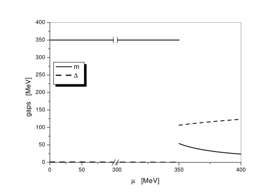
Figure 1: The constituent quark mass $m$ (solid line) and the color gap $\Delta$ (dashed line) as functions of the chemical potential $\mu$.

III Mesons and diquarks in dense quark matter

We are now interested in the investigation of the modification of meson and diquark masses in dense and cold quark matter with the color symmetry broken because of the 2SC diquark condensation. In the vacuum ($T=0$, $\mu=0$), particle masses are obtained from propagator poles, or alternatively, from zeros of the one-particle irreducible (1PI) two-point Green’s functions. Since the Lorentz invariance is preserved in the vacuum, these functions in (Minkowski) momentum space depend on $p^{2}=p_{0}^{2}-\vec{p}^{2}$ only. The squared mass of the particle is thus equal to the value of $p^{2}$ where the corresponding two-point 1PI correlators (Green’s function) vanishes. Insofar as $p^{2}$ is a Lorentz invariant, one can, for simplicity, choose the rest frame ($\vec{p}=0$), put $p^{2}=p_{0}^{2}$ and then consider these correlators as functions of $p_{0}$ alone. On the contrary, in a dense medium, the Lorentz invariance is broken, so the two-point Green’s functions in momentum space should be treated as functions of two variables: $p_{0}$ and $\vec{p}^{2}$ (the rotational symmetry is presumably conserved). The zeros of 1PI two-point Green’s functions in the $p_{0}$ plane will determine the particle and antiparticle dispersion laws, i. e. the relations between their energy and three-momenta. In this case, the scalar particle mass is defined as the value of the particle energy at $\vec{p}=0$ (see, e. g. ruivo ). Recently, the Bethe-Salpeter equation approach has been used to obtain diquark masses in the 2SC phase of cold dense QCD at asymptotically large values of the chemical potential mirsh . There, the mass of the diquark was defined as the energy of a bound state of two virtual quarks in the center of mass frame, i. e. in the rest frame for the whole diquark. Let us note here that just this quantity is measured on the lattice, where it is given by the exponential fall-off of the particle propagator at large Euclidean time (see, e. g., hands ). Similarly as in ruivo ; ratti and in numerous other papers, we shall denote, in the following, the rest frame energy of a composite scalar particle (meson or diquark), moving in a dense medium, as “mass”. (In general, the values of the mass depend on the chemical potential.)

Any 1PI Green’s function can be found from the effective action $S_{\rm eff}$, which up to second order in boson fields has the form

$$S_{\rm eff}=\frac{1}{2}\sum_{X,Y}\int d^{4}xd^{4}yX(x)\Pi_{XY}(x,y)Y(y)+\cdots,$$

where $X,Y=\pi_{a},\,\sigma,\,\Delta^{*}_{A},\,\Delta_{B}$, and $\Pi_{XY}(x,y)$ is the coordinate representation of the 1PI Green’s function for the fields $X,Y$. Instead of employing functional integration to get $S_{\rm eff}$ and then $\Pi_{XY}$, we shall use implicitly Feynman diagrams. Starting from the Lagrangian (6), one can expand the resulting effective action $S_{\rm eff}$ in a power series of meson and diquark fluctuations. Keeping there only the second order contributions, we immediately obtain the 1PI two-point correlators in the one-loop approximation. By considering this functions as functions of $p_{0}$ at zero three-momentum ($\vec{p}=0$), we shall next analyze their zeros which, as explained above, will give the masses of resonances.

III.1 Pion mass

Let us begin with the calculation of the pion mass. In the momentum representation, the 1PI two-point function $\Pi_{\pi_{a}\pi_{b}}(P)$ for the pion has the following form (all calculations are performed in the rest frame, $P=(p_{0},0,0,0)$ )

$$\Pi_{\pi_{a}\pi_{b}}(P)=-\frac{\delta^{ab}}{2G_{1}}+\frac{i}{2}\int\frac{d^{4}q}{(2\pi)^{4}}\mathrm{Tr}\left[S(P+q)\Gamma_{\pi}^{a}S(q)\Gamma_{\pi}^{b}\right].$$ (19)

Here, the vertex of the pion-quark interaction is given by the 2$\times$2 matrix $\Gamma_{\pi}^{a}=\left(\begin{array}[c]{ll}i\gamma_{5}\tau_{a}{}&0\\ 0{}&i\gamma_{5}\tau_{a}^{t}\end{array}\right)$. The first term in the right hand side of (19) is the tree contribution from Lagrangian (6), the second term arises from the one-loop diagram with two pion legs. After intermediate trace calculations, this function takes the form

$$\Pi_{\pi_{a}\pi_{b}}(P)=-\frac{\delta_{ab}}{2G_{1}}+16i\delta_{ab}\int\frac{d^{4}q}{(2\pi)^{4}}\frac{q_{0}(p_{0}+q_{0})-E^{+}E^{-}-\Delta^{2}}{D_{-}(q_{0})D_{+}(p_{0}+q_{0})}+$$

$$\qquad+8i\delta_{ab}\int\frac{d^{4}q}{(2\pi)^{4}}\frac{q_{0}(p_{0}+q_{0})-E^{+}E^{-}}{[(p_{0}+q_{0})^{2}-(E^{+})^{2}][(q_{0})^{2}-(E^{-})^{2}]}.$$ (20)

Implementing the imaginary-time formalism, as described in the end of the previous section (see also Appendix A for details), we reduce eq. (20) to three-dimensional integration in momentum space

$$\Pi_{\pi_{a}\pi_{b}}(P)=-\frac{\delta_{ab}}{2G_{1}}+8\delta_{ab}\int\frac{d^{3}q}{(2\pi)^{3}}\frac{E_{\Delta}^{+}E_{\Delta}^{-}+E^{+}E^{-}+\Delta^{2}}{E_{\Delta}^{+}E_{\Delta}^{-}}\frac{E_{\Delta}^{+}+E_{\Delta}^{-}}{(E_{\Delta}^{+}+E_{\Delta}^{-})^{2}-p_{0}^{2}}+$$

$$\qquad+16\delta_{ab}\int\frac{d^{3}q}{(2\pi)^{3}}\frac{\theta(E-\mu)E}{4E^{2}-p_{0}^{2}}\equiv\delta_{ab}\Pi_{\pi\pi}(p_{0}).$$ (21)

Then, up to a sign, the pion unnormalized propagator equals $(\Pi_{\pi_{a}\pi_{b}}(P))^{-1}$, whose pole in $p_{0}$ is given by the zero of the function $\Pi_{\pi\pi}(p_{0})$ from (21). We have searched for the roots of the equation $\Pi_{\pi\pi}(p_{0})=0$ numerically; the results for the pion mass $M_{\pi}$ at various $\mu$ are plotted in Fig. 2. A similar behavior of the pion mass in the Cooper pairing phase of a dense quark matter was found in ratti in the framework of a two-colored NJL model.

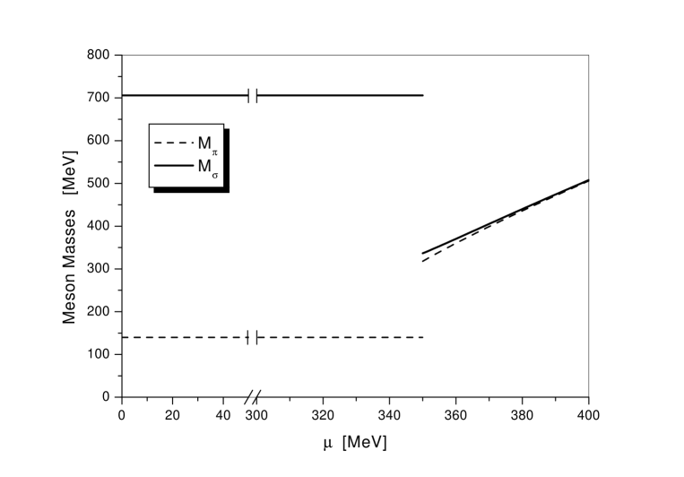
Figure 2: The masses of the $\sigma$-meson (solid line) and pion (dashed line) as functions of $\mu$.

In the color symmetric phase, the pion mass is below the threshold for the pion decay to a quark-antiquark pair, and the pion, therefore, is almost stable (only electroweak decay channels are allowed). Moreover, we have found that in the 2SC phase the pion is also an almost stable particle. This conclusion is supported by the following arguments. On the one hand, the pion cannot decay into a red/green quark-antiquark pair, since $M_{\pi}$ is less than the minimal energy $E_{\text{min}}=\sqrt{(\mu-m)^{2}+|\Delta|^{2}}+\sqrt{(\mu+m)^{2}+|\Delta|^{2}}$ that is necessary to create these particles (evidently, $E_{\text{min}}$ is the value of $E_{\Delta}^{-}+E_{\Delta}^{+}$ (see eq. (12) and the text after it) at $E=m$). On the other hand, the decay of a pion into a pair of blue quark-antiquark is also forbidden: i) Since all states with $E<\mu$ are occupied by quarks from the medium, the pion cannot decay into a blue quark with such values of $E$ because of the Pauli blocking, i.e. the analogy to the Mott effect. ii) In the region $E\geq\mu$, the energy of a blue quark-antiquark pair $(E^{-}+E^{+})$ takes its least value $E_{\text{min}}=2\mu$ at $E=\mu$, so the pion decay is again impossible, since $M_{\pi}<2\mu$. As a consequence, the pion is almost stable in the 2SC phase, too.

III.2 Mixing of $\sigma$-$\Delta_{2}$ in the 2SC phase. Scalar meson mass

An investigation of the 1PI Green’s functions $\Pi_{\sigma X}(P)$ with $P=(p_{0},0,0,0)$ for the fields $X=\Delta^{*}_{A},\Delta_{B}$ shows that in the 2SC phase the $\sigma$-meson is mixed with the $\Delta_{2}$ diquark. (At $\mu>\mu_{c}$, such a mixing occurs in the NJL model with two-colored quarks ratti , too. Moreover, as our preliminary results show, the mixing is present even if the condition of color neutrality of the 2SC phase is imposed.) The mass of the $\sigma$-meson in this case is given by the solution of the equation ${\rm det}(\Pi)=0$ where $\Pi(P)$ is the 3$\times$3 matrix

$$\Pi(P)=\left(\begin{array}[c]{lll}\Pi_{\sigma\sigma}(P)~{},&\Pi_{\sigma\Delta_{2}}(P),&\Pi_{\sigma\Delta^{*}_{2}}(P)\\ \Pi_{\Delta_{2}\sigma}(P),&\Pi_{\Delta_{2}\Delta_{2}}(P),&\Pi_{\Delta_{2}\Delta^{*}_{2}}(P)\\ \Pi_{\Delta^{*}_{2}\sigma}(P),&\Pi_{\Delta^{*}_{2}\Delta_{2}}(P),&\Pi_{\Delta^{*}_{2}\Delta^{*}_{2}}(P)\end{array}\right).$$ (25)

(Up to a sign, $\Pi(P)$ is the inverse propagator matrix for the $\sigma$-meson and $\Delta^{*}_{2}$, $\Delta_{2}$ diquarks.) After tedious but straightforward calculations, similar to those in the pion case, we get

$$\Pi_{\sigma\sigma}(P) = -\frac{1}{2G_{1}}+16\Delta^{2}m^{2}\int\frac{d^{3}q}{(2\pi)^{3}E^{2}}\,\left\{\frac{1}{E_{\Delta}^{+}[4(E_{\Delta}^{+})^{2}-p_{0}^{2}]}+\frac{1}{E_{\Delta}^{-}[4(E_{\Delta}^{-})^{2}-p_{0}^{2}]}\right\}+$$ (26)

$$+ 8\int\frac{d^{3}q}{(2\pi)^{3}}\,\frac{\vec{q}^{2}}{E^{2}}\,\frac{E_{\Delta}^{+}E_{\Delta}^{-}+E^{+}E^{-}+\Delta^{2}}{E_{\Delta}^{+}E_{\Delta}^{-}}\,\frac{E_{\Delta}^{+}+E_{\Delta}^{-}}{(E_{\Delta}^{+}+E_{\Delta}^{-})^{2}-p_{0}^{2}}+16\int\frac{d^{3}q}{(2\pi)^{3}}\,\frac{\vec{q}^{2}}{E}\,\frac{\theta(E-\mu)}{4E^{2}-p_{0}^{2}},$$

$$\Pi_{\sigma\Delta_{2}}(P) = \Pi_{\Delta^{*}_{2}\sigma}(P)=\Pi_{\sigma\Delta^{*}_{2}}(-P)=\Pi_{\Delta_{2}\sigma}(-P)=$$ (27)

$$= 4m\Delta\int\frac{d^{3}q}{(2\pi)^{3}}\left\{\frac{2E^{+}+p_{0}}{EE_{\Delta}^{+}[p_{0}^{2}-4(E_{\Delta}^{+})^{2}]}+\frac{2E^{-}-p_{0}}{EE_{\Delta}^{-}[p_{0}^{2}-4(E_{\Delta}^{-})^{2}]}\right\},$$

$$\Pi_{\Delta_{2}\Delta_{2}}(P) = \Pi_{\Delta^{*}_{2}\Delta^{*}_{2}}(P)=4\Delta^{2}I_{0}(p_{0}^{2}),~{}~{}~{}~{}~{}~{}~{}\Pi_{\Delta_{2}\Delta^{*}_{2}}(P)=\Pi_{\Delta^{*}_{2}\Delta_{2}}(-P)=$$ (28)

$$= -\frac{1}{4G_{2}}+I_{\Delta}+(4\Delta^{2}-2p_{0}^{2})I_{0}(p_{0}^{2})+4p_{0}I_{1}(p_{0}^{2}),$$

where $I_{\Delta}$ is given by (18), $I_{0}(p_{0}^{2})=A_{+}+A_{-}$, $I_{1}(p_{0}^{2})=B_{+}-B_{-}$, and

$$A_{+}=\int\frac{d^{3}q}{(2\pi)^{3}}\frac{1}{E_{\Delta}^{+}[p_{0}^{2}-4(E_{\Delta}^{+})^{2}]},~{}~{}~{} ~{}~{}~{}A_{-}=\int\frac{d^{3}q}{(2\pi)^{3}}\frac{1}{E_{\Delta}^{-}[p_{0}^{2}-4(E_{\Delta}^{-})^{2}]},$$ (29)

$$B_{+}=\int\frac{d^{3}q}{(2\pi)^{3}}\frac{E^{+}}{E_{\Delta}^{+}[p_{0}^{2}-4(E_{\Delta}^{+})^{2}]},~{}~{}~{} ~{}~{}~{}B_{-}=\int\frac{d^{3}q}{(2\pi)^{3}}\frac{E^{-}}{E_{\Delta}^{-}[p_{0}^{2}-4(E_{\Delta}^{-})^{2}]}.$$ (30)

(The formulas (26)–(28) are valid both in the 2SC ($\Delta\neq 0$) and in the color symmetric ($\Delta=0$) phases. In the 2SC phase, the 1PI Green’s functions $\Pi_{\Delta_{2}\Delta^{*}_{2}}(P)$, $\Pi_{\Delta^{*}_{2}\Delta_{2}}(P)$ (28) get a more simple form if one uses the identity $1=4G_{2}I_{\Delta}$ following from the gap equations (see eq. (18)).) In the general case ($m\neq 0$, $\Delta\neq 0$), the equation ${\rm det}(\Pi)=0$ has a rather complicated form. Fortunately, in the color symmetric phase with $\Delta=0$, i. e. at $\mu<\mu_{c}$, the nondiagonal terms $\Pi_{\sigma X}(P)$ ($X=\Delta^{*}_{2},\Delta_{2}$) in (25), which are responsible for the mixing of the $\sigma$-meson and the diquark, vanish because they are proportional to $\Delta$. Therefore, the $\sigma$-meson mass decouples from the diquark spectrum and is found from the equation

$$\Pi_{\sigma\sigma}(P)=0.$$ (31)

On the other hand, in the 2SC phase (see Fig. 1), the constituent quark mass $m$ is small (or even equal to zero if $m_{0}=0$) in the 2SC phase (see Fig. 1), so one can ignore the nondiagonal elements $\Pi_{\sigma\Delta_{2}}(P)$, $\Pi_{\sigma\Delta^{*}_{2}}(P)$ in $\Pi$ because they are negligibly small (as proved a posteriori by numerical computations), and the $\sigma$-meson mass $M_{\sigma}$ is again found from eq. (31). The numerical solution of eq. (31) is presented in Fig. 2, where one can see that both $\sigma$- and $\pi$-meson masses are increasing functions of $\mu$ in the 2SC phase. At the same time, the difference between $M_{\sigma}$ and $M_{\pi}$ decreases with $\mu$; $\delta M=M_{\sigma}-M_{\pi}$ becomes negligible at sufficiently high $\mu$, which is understood as an evidence of the chiral symmetry restoration. The decrease of the dynamical quark mass $m$ at large $\mu$ (see Fig. 1) is also in accordance with this conclusion.

Finally, we would like to note that the $\sigma$-meson is almost stable in the 2SC phase for the same reason which was explained in the last paragraph of the previous section for the case of the pion.

III.3 Diquark masses

In dense quark matter (at nonzero (baryon) chemical potential), the symmetry of the Lagrangian under charge conjugation is violated by the chemical potential. As a consequence, the mass spectrum of diquarks can split, and diquarks will differ from antidiquarks not only by charge but also by mass.

III.3.1 Diquark masses in the color symmetric phase ($\Delta=0$)

In the color symmetric phase ($\mu<\mu_{c}=350$ MeV), the ground state of the quark matter is described by $\Delta=0$, and there is no mixing between diquarks in the one-loop approximation. Therefore, one can, e. g., consider the propagator of $\Delta^{*}_{2},\Delta_{2}$ alone. It follows from eq. (28) that $\Pi_{\Delta_{2}\Delta_{2}}(P)=$ $\Pi_{\Delta^{*}_{2}\Delta^{*}_{2}}(P)=0$ at $\Delta=0$, and one needs only

$$\Pi_{\Delta_{2}\Delta^{*}_{2}}(P)=\Pi_{\Delta^{*}_{2}\Delta_{2}}(-P)=-\frac{1}{4G_{2}}-16\int\frac{d^{3}q}{(2\pi)^{3}}\frac{E}{(p_{0}+2\mu)^{2}-4E^{2}}\equiv-\frac{1}{4G_{2}}+F(\epsilon).$$ (32)

Here, $P=(p_{0},0,0,0)$, $\epsilon=(p_{0}+2\mu)^{2}$. (In obtaining (32), we have used the relation $\mu<m$, i. e. $E^{-}>0$, which is true for the color symmetric phase.) Then, the 2$\times$2 inverse propagator matrix $\mathcal{G}^{-1}_{2}(P)$ in the $\Delta^{*}_{2},\Delta_{2}$-sector of the NJL model has the form

$$\mathcal{G}^{-1}_{2}(P)=-\left(\begin{array}[c]{cc}0~{}~{},&\Pi_{\Delta_{2}\Delta^{*}_{2}}(P)\\ \Pi_{\Delta^{*}_{2}\Delta_{2}}(P),&~{}0\end{array}\right).$$ (33)

Clearly, the mass spectrum is determined by the equation ${\rm det}(\mathcal{G}^{-1}_{2})=\Pi_{\Delta_{2}\Delta^{*}_{2}}(P)\Pi_{\Delta^{*}_{2}\Delta_{2}}(P)=0$, or by zeros of (32), where the function $F(\epsilon)$ is analytical in the whole complex $\epsilon$-plane, except for the cut $4m^{2}<\epsilon$ along the real axis. (In general, the function $F(\epsilon)$ is defined on a complex Riemann surface which is described by several sheets. However, a direct numerical computation based on eq. (32) gives its values in the first sheet only. To find a value on the rest of the Riemann surface, a special procedure of continuation is needed.) The numerical analysis of (32) in the first Riemann sheet shows that the equation $\Pi_{\Delta_{2}\Delta^{*}_{2}}(P)=\Pi_{\Delta^{*}_{2}\Delta_{2}}(-P)=0$ has a root ($\epsilon_{0}$) on the real axis ($0<\epsilon_{0}<4m^{2}$), providing us with the following massive diquark modes

$$M_{\Delta}=1.998m-2\mu,~{}~{}~{}~{}~{}M_{\Delta^{*}}=1.998m+2\mu.$$ (34)

We relate $M_{\Delta}$ in (34) to the mass of the diquark with the baryon number $B=2/3$ and $M_{\Delta^{*}}$ to the mass of the antidiquark with $B=-2/3$. (Qualitatively, a similar behavior of diquark and antidiquark masses vs. $\mu$ was obtained in ratti in the NJL model for two-colored quarks.) It follows from (34) that in the vacuum ($\mu=0$) the diquark/antidiquark mass is $\sim 2m$. Clearly, in the color symmetric phase at $\mu\neq 0$ both quantities $M_{\Delta}$ and $M_{\Delta^{*}}$ from (34) are nothing else but the rest frame excitation energies for a diquark and antidiquark, respectively.

In the color symmetric phase for $\mu<m$ the diquarks and antidiquarks are stable. Indeed, the diquark mass $M_{\Delta}$ is smaller here than the energy $2(m-\mu)$ necessary to create a pair of free quarks. Finally, due to the underling color $\rm SU(3)_{c}$ symmetry, the previous statement is valid also for $\Delta^{*}_{5},\Delta_{5}$ and $\Delta^{*}_{7},\Delta_{7}$. As a result, we have a color antitriplet of diquarks with the mass $M_{\Delta}$ (34) as well as a color triplet of antidiquarks with the mass $M_{\Delta^{*}}$. The results of numerical computations are presented in Fig. 3: the solid line shows the behavior of the antidiquark triplet mass $M_{\Delta^{*}}$ in the region of $\mu<\mu_{c}=350$ MeV whereas the dashed line corresponds to the antitriplet.

In our analysis, we have used the constraint $G_{2}=3G_{1}/4$, thereby fixing the constant $G_{2}$ through $G_{1}$. It is useful, however, to discuss now the influence of $G_{2}$ on diquark masses. Indeed, it is clear from (32) that the root $\epsilon_{0}$ lies inside the interval $0<\epsilon_{0}<4m^{2}$ only if $G_{2}^{*}<G_{2}<G_{2}^{**}$, where $G_{2}^{*}$ and $G_{2}^{**}$ are defined by

$$G_{2}^{*} \equiv \frac{1}{4F(4m^{2})}=\frac{\pi^{2}}{4\left[\Lambda\sqrt{m^{2}+\Lambda^{2}}+m^{2}\ln((\Lambda+\sqrt{m^{2}+\Lambda^{2}})/m)\right]},$$

$$G_{2}^{**} \equiv \frac{1}{4F(0)}=\frac{\pi^{2}}{4\left[\Lambda\sqrt{m^{2}+\Lambda^{2}}-m^{2}\ln((\Lambda+\sqrt{m^{2}+\Lambda^{2}})/m)\right]}=\frac{3mG_{1}}{2(m-m_{0})}.$$ (35)

In this case, there are stable diquarks and antidiquarks in the color symmetric phase. The behavior of their masses qualitatively resembles that given by eqs. (34). For a rather weak interaction in the diquark channel ($G_{2}<G_{2}^{*}$), $\epsilon_{0}$ runs onto the second Riemann sheet, and unstable diquark modes (resonances) appear. Unlike this, a sufficiently strong interaction in the diquark channel ($G_{2}>G_{2}^{**}$) pushes $\epsilon_{0}$ towards the negative semi-axis, i. e. $(p_{0}+2\mu)^{2}<0$. The latter indicates a tachyon singularity in the diquark propagator, evidencing that the color symmetric ground state is not stable. Indeed, as it has been shown in ek , at a very large $G_{2}$ the color symmetry is spontaneously broken even at a vanishing chemical potential.

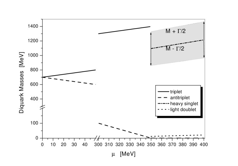
Figure 3: The masses of diquarks. At $\mu<\mu_{c}=350$ MeV, six diquark states are splitted into a (color)triplet of heavy states with mass $M_{\Delta^{*}}$ (solid line) and an anti-triplet (dashed line) of light states with mass $M_{\Delta}$. In the 2SC phase ($\mu>\mu_{c}$), one observes 3 massless diquarks (dashed line): a doublet of light diquarks with the mass $M_{\mbox{\tiny light}}$ (dotted line) and a heavy singlet state with the mass $M$ (dash-dotted line). The shaded rectangular displays the width of the heavy singlet resonance; its upper border is half-width higher than the mass and the bottom border is half-width lower.

III.3.2 Diquark masses in the 2SC phase ($\Delta\neq 0$)

Let us now focus on the masses of $\Delta^{*}_{2},\Delta_{2}$-fields. As we have already shown in Section III.2, these diquarks are mixed with the $\sigma$-meson in the 2SC phase because of the nonvanishing terms $\Pi_{\sigma\Delta_{2}}(P)$ and $\Pi_{\sigma\Delta^{*}_{2}}(P)$ in the matrix $\Pi(P)$ (25). However, keeping in mind that the constituent quark mass $m$ is small in the color superconducting phase, one can ignore this mixing. The problem becomes, thereby, drastically simplified, and one just has to calculate the determinant of

$$\mathcal{G}^{-1}_{2}(P)=-\left(\begin{array}[c]{cc}\Pi_{\Delta_{2}\Delta_{2}}(P),&\Pi_{\Delta_{2}\Delta^{*}_{2}}(P)\\ \Pi_{\Delta^{*}_{2}\Delta_{2}}(P),&\Pi_{\Delta^{*}_{2}\Delta^{*}_{2}}(P)\end{array}\right)$$ (36)

and equate it to zero. The resulting equation will determine the masses of $\Delta^{*}_{2},\Delta_{2}$. Taking the expressions for the matrix elements in (36) from eqs. (27) and (28) and using the relation $1=4G_{2}I_{\Delta}$ (valid in the 2SC phase only), we get the mass equation

$${\rm det}(\mathcal{G}^{-1}_{2})\equiv 4p_{0}^{2}\big{\{}(p_{0}^{2}-4\Delta^{2})I_{0}^{2}(p_{0}^{2})-4I_{1}^{2}(p_{0}^{2})\big{\}}=0.$$ (37)

It has the apparent solution $p_{0}^{2}=0$ corresponding to a Nambu–Goldstone (NG) boson. The second solution of (37) exists on the second Riemann sheet for $p_{0}^{2}$ only (see Appendix B).

Near a zero, the determinant ${\rm det}(\mathcal{G}^{-1}_{2})$ can be approximated by

$${\rm det}(\mathcal{G}^{-1}_{2})\sim p_{0}^{2}-M^{2}+iM\Gamma.$$ (38)

Here, $M$ is the mass of the resonance, and $\Gamma$ is its width. Let $\tilde{p}_{0}$ be a root of the equation

$$\tilde{p}_{0}^{2}-M^{2}+iM\Gamma=0,$$ (39)

the mass and width are then given by

$$M=\sqrt{\mbox{Re}\,\tilde{p}_{0}^{2}},\qquad\Gamma=-\frac{\mbox{Im}\,\tilde{p}_{0}^{2}}{M}.$$ (40)

For a small width, we can write for the root of eq. (39)

$$\tilde{p}_{0}\approx M-i\frac{\Gamma}{2}.$$ (41)

The appearance of the imaginary part in (41) is a consequence of the fact that this diquark is a resonance in the 2SC phase and can decay into free quarks. Our numerical estimates for $M$ and $\Gamma$ at various $\mu$ are plotted in Fig. 3. The dot-dashed line corresponds to $M$, while the width is given by the hight of the shaded block, half-width up and half-width down.

We would like to point out here that both the resonance and the above mentioned NG-boson are color singlets with respect to $\rm SU(2)_{c}$. Since the obtained mass $M$ is much greater than even twice the energy $\sqrt{(m+\mu)^{2}+|\Delta|^{2}}$ necessary for creating an antiquark in the 2SC phase, there is no wonder that this diquark mode is unstable, unlike the pion and $\sigma$, which are stable due to the Mott effect.

A detailed investigation of the diquark masses in the $\Delta^{*}_{5},\Delta_{5}$- and $\Delta^{*}_{7},\Delta_{7}$ sectors has already been done in our previuos paper bekvy . It was found there that in each of these sectors there was an NG-boson as well as a light diquark excitation with the same mass $M_{\mathrm{light}}$ proportional to the color-8 charge density of the quark matter in the 2SC ground state. So, we can conclude that, in total, there is an abnormal number of three NG-bosons in the theory, instead of expected five (Since $\rm SU(3)_{c}$ is spontaneously broken down to $\rm SU(2)_{c}$, five group generators affect the diquark condensate, and therefore, five NG bosons should appear, according to the Goldstone theorem). This entails absence of baryon superfluidity in the 2SC phase (see also the discussions in miransky ; ms , where the effect of NG-boson deficiency was observed in other relativistic models with broken Lorentz invariance). The light diquarks form a stable $\rm SU(2)_{c}$-doublet with the mass $M_{\mathrm{light}}$ whose dependence on $\mu$ is also shown in Fig. 3 (dotted line).

IV Summary and discussion

In the present paper, we have investigated the mass spectrum of meson and diquark excitations in cold dense quark matter. We started from a low-energy effective model of the Nambu–Jona-Lasinio type for quarks of two flavors including a single quark chemical potential, for simplicity. Despite of the lack of confinement, this model quite satisfactorily describes the masses and dynamics of light mesons in normal quark matter (at rather small values of chemical potential). Since the investigation of color superconductivity became popular nowadays, NJL models have also been widely used to explore, in particular, the quark matter phase diagram for intermediate densities, i. e. under conditions where all other approaches fail.

Using the one-loop approximation, we calculated two-point correlators of mesons and showed that the masses of $\pi$- and $\sigma$-mesons grow with the quark chemical potential in the 2SC phase (see Fig. 2). The mass difference between them vanishes at asymptotically large $\mu$, in accordance with chiral symmetry restoration. Moreover, these mesons are stable in the 2SC phase due to the Mott effect. As far as we know, the properties of $\pi$- and $\sigma$-mesons in the 2SC phase have not been discussed in the literature before.

In the diquark sector, the situation is more involved in the 2SC phase. Indeed, when the color $\rm SU(3)_{c}$-symmetry is spontaneously broken down to $\rm SU(2)_{c}$, one naturally expects five (massless) NG bosons to appear. Unlike this, one finds only three massless bosonic excitations bekvy : a color singlet and a color doublet (due to the residual $\rm SU(2)_{c}$ symmetry). In spite of the abnormal number of NG-bosons (notice that each member of the doublet has a quadratic dependence of its energy on three-momentum when it is almost at rest), there is no contradiction with the NG-bosons counting nc . Apart from this, there are also two light and one heavy diquark modes (see Fig. 3). The first two are stable, whereas the last one is a resonance with finite width, and its 1PI Green’s function possesses a zero in the second Riemann sheet for the energy variable.

We have also found that the antidiquark masses exceed those of the diquarks in the color symmetric phase (for $\mu<\mu_{c}=350$ MeV). This splitting of the masses is explained by the violation of $C$-parity (charge conjugation) in the presence of a chemical potential. In contrast, at $\mu=0$ the model is $C$-invariant and all diquarks and antidiquarks have the same mass which is slightly lower than two dynamical quark masses, $\sim$700 MeV. Our result for the diquark mass in the vacuum ($\mu=0$) is in agreement with maris , where the value as large as $\sim 800$ MeV was claimed to follow from QCD via solving a Bethe–Salpeter equation in the rainbow-ladder approximation.

Of course, all observable particles render themselves as colorless objects in the hadronic phase, and the diquarks are expected to be confined, as they are not $\rm SU(3)_{c}$ color singlets. Nevertheless, one may look at our and other related results on diquark masses as an indication of the existence of rather strong quark-quark correlations inside baryons, which might help to explain baryon dynamics. Some lattice simulations reveal strong attraction in the diquark channel wk with a diquark mass $\sim$600 MeV. Recently, in jw , the mass and extremely narrow width, as well as other properties, of the pentaquark $\Theta^{+}$ were explained just on the assumption that it is composed of an antiquark and two highly correlated $ud$-pairs. At present time, the nature of the mechanism which may entail strong attraction of quarks in diquark channels is actively discussed both in the nonperturbative QCD and in other models (see, e. g. ripka and references therein).

Finally, let us comment on the fact that we considered in this paper only a single chemical potential $\mu$ (common for all quarks). Obviously, in such a simplified approach, the 2SC quark matter is neither color nor electrically neutral, as it would be expected for realistic situations like, for example, in the cores of compact stars. In order to study color superconductivity in the case of neutral matter, one has to study more complex NJL models including several new chemical potentials neutr ). Despite this drawback, the chosen simplified approach, nevertheless, seems to us interesting enough to get some deeper understanding of the dynamics of mesons and diquarks in the color symmetric and 2SC phases of cold dense quark matter. A generalization of this approach to more sophisticated NJL models including several chemical potentials is presently under investigation.

Appendix A Loop integrals at $T\neq 0$ and $\mu\neq 0$

To evaluate loop integrals, we use in our paper the imaginary-time formalism (see, e. g. kap ). First of all, it is supposed that the system is in the thermodynamic equilibrium with a thermal bath of some temperature $T$. As usual, to study a hot and dense system, one has to calculate thermal Green’s functions (TGF), which are periodic (for each boson field) and antiperiodic (for each fermion field) functions of imaginary time. Their Fourier images are, thereby, functions defined at discrete points in the imaginary axis $p_{0}=i\omega_{n},\,n=0,\pm 1,\pm 2,\ldots$, with $\omega_{n}$ being Matsubara frequencies. When calculating a loop diagram, one has to sum over $q_{0}=i\omega_{n}=i2n\pi T$ for bosons and $q_{0}=i\omega_{n}=i(2n+1)\pi T$ for fermions. In accordance with this, the integration over $q_{0}$ in (14), (15), etc is to be performed in two steps: First, all momenta are considered in Euclidean metric, and a sum over Matsubara frequencies is performed. Then, the limit $T\to 0$ is reached and the resulting TGF are continued in the complex plane to the real axis, which corresponds to their definition in Minkowski metric. As a result, we have then for 1PI Green’s functions the formulas where the four-dimensional integration is reduced to three dimensions.

Let us explain the scheme, briefly outlined above, in a bit more details. First, we delay the three-dimensional integration until the end of the calculations, and consider only one-dimensional $q_{0}$-integrals. Only one such integration comes from each diagram in the one-loop approximation for the 1PI Green’s functions with two bosonic legs, and it can be represented as

$$F(p_{0})=\int\frac{dq_{0}}{2\pi i}f(q_{0},\vec{q};p_{0}),$$ (42)

where the function $f(q_{0},\vec{q};p_{0})$ is a product of vertices and quark propagators from a one-loop diagram, while the external three-momentum in each diagram is supposed to be zero, $\vec{p}=0$. The dependence of the function $F(p_{0})$ on the momentum $\vec{q}$ is implied, however, we do not write $\vec{q}$ explicitly, since only the dependence on $p_{0}$ is important for the moment.

At $T\neq 0$, one would obtain in the right hand side of (42) a sum over the fermionic Matsubara frequencies $\omega_{n}=(2n+1)\pi T$ instead of the integral. Let us denote the result of the sum by the function $F_{T}(p_{0})$. It is defined only at the values of $p_{0}=i\nu_{k}=i2k\pi T$, corresponding to bosonic Matsubara frequencies, because each external line in the implied one-loop diagram corresponds to a boson. The result looks like

$$F_{T}(i\nu_{k})=T\sum_{n=-\infty}^{\infty}f(i\omega_{n},\vec{q};i\nu_{k}).$$ (43)

Let us assume that the function $f(\omega,\vec{q};i\nu_{k})$ falls sufficiently quickly in any direction on the complex $\omega$-plane and contains only simple poles everywhere, except for the imaginary axis. In this case, using the Cauchy theorem, one can replace the sum over Matsubara frequencies in (43) by ”closed” contour integrals and obtains

$$F_{T}(i\nu_{k})=T\!\sum_{n=-\infty}^{\infty}f(i\omega_{n},\vec{q};i\nu_{k})=\frac{1}{2}\oint\limits_{C_{1}+C_{2}}\frac{d\omega}{2\pi i}f(\omega,\vec{q};i\nu_{k})\tanh\left(\frac{\omega}{2T}\right),$$ (44)

where the contour $C_{1}$ is just the straight line from $-i\infty+\epsilon$ to $i\infty+\epsilon$, and $C_{2}$ is the straight line from $i\infty-\epsilon$ to $-i\infty-\epsilon$. The contour integral in (44) is indeed the sum of two integrals: $C_{1}$ and $C_{2}$. Both $C_{1}$ and $C_{2}$ can be closed by infinite arcs in the right and left halves of the complex plane because the integration along these arcs vanishes if the integrands fall quickly enough near infinity. As a consequence, we can then integrate along the closed contours $\tilde{C}_{1}$ and $\tilde{C}_{2}$. As the integrand was supposed to have only simple poles, the Cauchy theorem immediately gives us the result of integrations via a sum of residues of the integrand at these poles, which are determined by the poles of the quark propagator. It is important to keep in mind before taking the limit $T\to 0$ that $\nu_{k}=2k\pi T$. The point is that after the calculation of all residues the frequency $i\nu_{k}$ will appear in the argument of the hyperbolic tangent $\tanh(\omega/2T)$, which is periodic on the imaginary axis and the period is just equal to $i2\pi T$. Therefore, the tangent does not depend on $i\nu_{k}$, and one can put $\nu_{k}=0$ in its argument. After this, one can reach the limit $T\to 0$ and continue the function $F_{T}|_{T=0}$ to real energies $p_{0}$, which is formally obtained through the substitution $\nu_{k}\to-ip_{0}$ in the rest of the expression.

We follow the scheme explained above to calculate the tadpole contributions (see (13)), which do not depend on external momenta. Let us consider, as an example, the one-loop tadpole contribution for $\langle\Delta^{*}_{2}(x)\rangle$, which is nothing else than the right hand side of (15). Replacing the $q_{0}$-integral by a sum over Matsubara frequencies $\omega_{n}=(2n+1)\pi T$ (see (16)) and following other steps, we obtain

$$I_{\Delta}(T) = -4T\sum_{n=-\infty}^{\infty}\int\frac{d^{3}q}{(2\pi)^{3}}\left\{\frac{1}{D_{+}(i\omega_{n})}+\frac{1}{D_{-}(i\omega_{n})}\right\}=$$ (45)

$$= -2\oint\limits_{\tilde{C}_{1}+\tilde{C}_{2}}\frac{d\omega}{2\pi i}\tanh\left(\frac{\omega}{2T}\right)\int\frac{d^{3}q}{(2\pi)^{3}}\left\{\frac{1}{D_{+}(\omega)}+\frac{1}{D_{-}(\omega)}\right\},$$

where $D_{\pm}(\omega)$ are defined by (12), and the two clockwise contours $\tilde{C}_{1}$ and $\tilde{C}_{2}$ enclose the right and left halves of the complex $\omega$-plane. The integrand in (45) has only four simple poles at $\omega=\pm E^{+}_{\Delta}$ and $\omega=\pm E^{-}_{\Delta}$. Finally, we replace the integral in (45) by a sum of the residues at these poles, multiplied by $2\pi i$ (according to the Cauchy theorem), and take the limit $T\to 0$. This gives for $I_{\Delta}=\lim_{T\to 0}I_{\Delta}(T)$ the expression displayed in the right hand side of (18).

Appendix B Searching for the resonance solution of eq. (37)

The nontrivial solution of (37) obeys the equation

$$(zI_{0}-2I_{1})(zI_{0}+2I_{1})=0,$$ (46)

where $z^{2}=p_{0}^{2}-4\Delta^{2}$ and $I_{0,1}$ are given by (28). Below we shall ignore, for simplicity, the dynamical quark mass (i. e. putting $m=0$), because we assume (and this assumption is a posteriori corroborated by numerical calculations of the heavy diquark mass both for $m=0$ and $m\neq 0$) that this simplification does not strongly affect our results. First of all, we integrate over the angles in (29) and (30) and introduce a new variable $y=(E+\mu)^{2}$, instead of the three-momentum, in the integrals $A_{+}$ and $B_{+}$ (recall that $E=|\vec{q}|$)

$$A_{+}=\frac{1}{4\pi^{2}}\int_{\mu^{2}}^{(\Lambda+\mu)^{2}}\frac{(\sqrt{y}-\mu)^{2}dy}{\sqrt{y}\sqrt{y+\Delta^{2}}[z^{2}-4y]},~{}~{}~{}B_{+}=\frac{1}{4\pi^{2}}\int_{\mu^{2}}^{(\Lambda+\mu)^{2}}\frac{(\sqrt{y}-\mu)^{2}dy}{\sqrt{y+\Delta^{2}}[z^{2}-4y]}.$$ (47)

Since

$$A_{-}=\int_{0}^{\mu}(\cdots)dE+\int_{\mu}^{\Lambda}(\cdots)dE,$$ (48)

one can introduce the new variables $\sqrt{y}=\mu-E$ and $\sqrt{y}=E-\mu$ for the first and second integrals of (48), respectively, and get

$$A_{-}=\frac{1}{4\pi^{2}}\int^{\mu^{2}}_{0}\frac{(\sqrt{y}-\mu)^{2}dy}{\sqrt{y}\sqrt{y+\Delta^{2}}[z^{2}-4y]}+\frac{1}{4\pi^{2}}\int^{(\Lambda-\mu)^{2}}_{0}\frac{(\sqrt{y}+\mu)^{2}dy}{\sqrt{y}\sqrt{y+\Delta^{2}}[z^{2}-4y]}$$ (49)

and

$$I_{0}=A_{+}+A_{-}=\frac{1}{4\pi^{2}}\int^{(\Lambda+\mu)^{2}}_{0}\frac{(\sqrt{y}-\mu)^{2}dy}{\sqrt{y}\sqrt{y+\Delta^{2}}[z^{2}-4y]}+\frac{1}{4\pi^{2}}\int^{(\Lambda-\mu)^{2}}_{0}\frac{(\sqrt{y}+\mu)^{2}dy}{\sqrt{y}\sqrt{y+\Delta^{2}}[z^{2}-4y]}.$$ (50)

In a similar way, one obtains

$$I_{1}=B_{+}-B_{-}=\frac{1}{4\pi^{2}}\int^{(\Lambda+\mu)^{2}}_{0}\frac{(\sqrt{y}-\mu)^{2}dy}{\sqrt{y+\Delta^{2}}[z^{2}-4y]}-\frac{1}{4\pi^{2}}\int^{(\Lambda-\mu)^{2}}_{0}\frac{(\sqrt{y}+\mu)^{2}dy}{\sqrt{y+\Delta^{2}}[z^{2}-4y]}.$$ (51)

The quantities $I_{0,1}$ are analytical functions of the complex variable $z^{2}\equiv a-ib$ on the whole complex plane, except for the cut $L$ on the real axis, defined by $0\leq z^{2}\leq(\Lambda+\mu)^{2}$ (the first Riemann sheet). A numerical processing of the integrals (50) and (51) gives the values of functions $I_{0}$ and $I_{1}$ on the first Riemann sheet only. But there is no solution for eq. (46) in the first Riemann sheet because the root of eq. (46) lies on the lower half-plane ($b>0$) of the second Riemann sheet, and in order to find it, we have to continue $I_{0}$ and $I_{1}$ to the second sheet. When $z^{2}$ crosses the cut $L$ downwards from the upper half of the first sheet, the integrals $I_{0}$ (50) and $I_{1}$ (51) become singular because of the apparent poles in the integrands. Since an integral does not change when the contour is being continuously transformed on the complex plane until it crosses a singularity of the integrand, we carefully deviate our contour on the complex $y$-plane to circumvent the singularity in a way shown in Fig. 4. When the contours $C_{1}$ and $C_{2}$ overlap each other, the sum of the integrals along them vanishes, and as a result, we obtain that $I_{0}$ and $I_{1}$ in the lower half-plane of the second Riemann sheet differ from (50) and (51) by an additional integral over the contour $C$ around the pole $z^{2}$ (see Fig. 4) which is equal to the residue of the integrand at $z^{2}$. Let us denote the continuations of $I_{0}$ and $I_{1}$ to the second Riemann sheet as $\tilde{I}_{0}$ and $\tilde{I}_{1}$. Then, one has

$$\tilde{I}_{0}=I_{0}-\frac{i(z^{2}+4\mu^{2})}{4\pi z\sqrt{z^{2}+4\Delta^{2}}},~{}~{}~{}~{}~{}~{}~{}\tilde{I}_{1}=I_{1}+\frac{iz\mu}{2\pi\sqrt{z^{2}+4\Delta^{2}}},$$ (52)

where $z=\sqrt{z^{2}}=a_{1}-ib_{1}$, with both $a_{1}$ and $b_{1}$ being real and positive: $a_{1}=\sqrt{\frac{1}{2}a+\frac{1}{2}\sqrt{a^{2}+b^{2}}}$, $b_{1}=b/\sqrt{2a+2\sqrt{a^{2}+b^{2}}}$; apart from, $\sqrt{z^{2}+4\Delta^{2}}=\tilde{a}_{1}-i\tilde{b}_{1}$, where $\tilde{a}_{1}=\sqrt{\frac{1}{2}(a+4\Delta^{2})+\frac{1}{2}\sqrt{(a+4\Delta^{2})^{2}+b^{2}}}$, $\tilde{b}_{1}=b/\sqrt{2(a+4\Delta^{2})+2\sqrt{(a+4\Delta^{2})^{2}+b^{2}}}$.

Let us now consider the function $F(z^{2})=\sqrt{z^{2}}I_{0}(z^{2})+2I_{1}(z^{2})$ (it is the second multiplier in (46)). Its continuation to the second Riemann sheet is $F\to\tilde{F}(z^{2})=\sqrt{z^{2}}\tilde{I}_{0}+2\tilde{I}_{1}=F(z^{2})-i(\sqrt{z^{2}}-2\mu)^{2}/(4\pi\sqrt{z^{2}+4\Delta^{2}})$. Numerical solution of the equation $\tilde{F}(z^{2})=0$ at various $\mu>\mu_{c}$ gives one root per one value of $\mu$: $z_{0}^{2}+4\Delta^{2}=M^{2}-iM\Gamma$. For example, if one puts $\Delta=115$ MeV, $\mu=350$ MeV and $\Lambda=618$ MeV, one gets the mass $M=1111$ MeV and the width $\Gamma=446$ MeV.

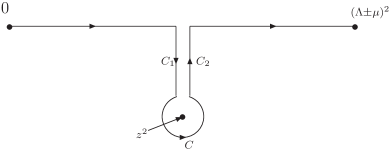
Figure 4: The deformation of the integration contour on the complex $y$-plane for the functions $I_{0},I_{1}$ when the parameter $z^{2}$ moves onto the lower half-plane of the second Riemann sheet.

References

- (1) Z. Fodor and S. D. Katz, JHEP 0203, 014 (2002); JHEP 0404, 050 (2004).
- (2) D. T. Son, Phys. Rev. D59, 094019 (1999); T. Schäfer and F. Wilczek, Phys. Rev. D60, 114033 (1999); R. D. Pisarski and D. H. Rischke, Phys. Rev. D61, 074017 (2000); D. K. Hong, V. A. Miransky, I. A. Shovkovy and L. C. Wijewardhana, Phys. Rev. D61, 056001 (2000); W. E. Brown, J. T. Liu and H.-C. Ren, Phys. Rev. D61, 114012 (2000).
- (3) Y. Nambu and G. Jona-Lasinio, Phys. Rev. 124, 246 (1961).
- (4) R. Rapp, T. Schäfer, E. V. Shuryak and M. Velkovsky, Ann. Phys. 280, 35 (2000); M. Alford, Ann. Rev. Nucl. Part. Sci. 51, 131 (2001); G. Nardulli, Riv. Nuovo Cim. 25N3, 1 (2002); T. Schäfer, hep-ph/0304281; M. Buballa, hep-ph/0402234.
- (5) M. Huang, hep-ph/0409167; I. A. Shovkovy, nucl-th/0410091.
- (6) E. V. Shuryak, hep-ph/0405066.
- (7) D. Blaschke, D. Ebert, K. G. Klimenko, M. K. Volkov and V. L. Yudichev, Phys. Rev. D70, 014006 (2004).
- (8) D. Ebert and M. K. Volkov, Yad. Fiz. 36, 1265 (1982); Z. Phys. C16, 205 (1983); M. K. Volkov, Annals Phys. 157, 282 (1984); D. Ebert and H. Reinhardt, Nucl. Phys. B271, 188 (1986); D. Ebert, H. Reinhardt and M. K. Volkov, Progr. Part. Nucl. Phys. 33, 1 (1994).
- (9) M. K. Volkov, Fiz. Elem. Chast. Atom. Yadra 17, 433 (1986).
- (10) T. Hatsuda and T. Kunihiro, Phys. Rept. 247, 221 (1994); S. P. Klevansky, Rev. Mod. Phys. 64, 649 (1992).
- (11) M. K. Volkov and V. L. Yudichev, Phys. Part. Nucl. 32S1, 63 (2001).
- (12) D. Ebert, L. Kaschluhn and G. Kastelewicz, Phys. Lett. B264, 420 (1991).
- (13) U. Vogl, Z. Phys. A337, 191 (1990); U. Vogl and W. Weise, Progr. Part. Nucl. Phys. 27, 195 (1991).
- (14) D. Ebert and L. Kaschluhn, Phys. Lett. B297, 367 (1992); D. Ebert and T. Jurke, Phys. Rev. D58, 034001 (1998); L. J. Abu-Raddad et al., Phys. Rev. C66, 025206 (2002).
- (15) H. Reinhardt, Phys. Lett. B244, 316 (1990); N. Ishii, W. Benz and K. Yazaki, Phys. Lett. B301, 165 (1993); C. Hanhart and S. Krewald, ibid. B344, 55 (1995).
- (16) V. P. Gusynin, V. A. Miransky and I. A. Shovkovy, Phys. Lett. B349, 477 (1995); A. Yu. Babansky, E. V. Gorbar and G. V. Shchepanyuk, Phys. Lett. B419, 272 (1998); A. S. Vshivtsev, M. A. Vdovichenko and K. G. Klimenko, Phys. Atom. Nucl. 63, 470 (2000); D. Ebert et al, Phys. Rev. D61, 025005 (2000); T. Inagaki, D. Kimura and T. Murata, Prog. Theor. Phys. 111, 371 (2004).
- (17) T. Inagaki, T. Muta and S. D. Odintsov, Mod. Phys. Lett. A8, 2117 (1993); Prog. Theor. Phys. Suppl. 127, 93 (1997); E. V. Gorbar, Phys. Rev. D61, 024013 (2000); Yu. I. Shilnov and V. V. Chitov, Phys. Atom. Nucl. 64, 2051 (2001).
- (18) D. K. Kim and I. G. Koh, Phys. Rev. D51, 4573 (1995); A. S. Vshivtsev, M. A. Vdovichenko and K. G. Klimenko, J. Exp. Theor. Phys. 87, 229 (1998); E. J. Ferrer, V. de la Incera and V. P. Gusynin, Phys. Lett. B455, 217 (1999); E. J. Ferrer and V. de la Incera, hep-ph/0408229.
- (19) M. Asakawa and K. Yazaki, Nucl. Phys. A504, 668 (1989); P. Zhuang, J. Hüfner and S. P. Klevansky, Nucl. Phys. A576, 525 (1994).
- (20) D. Ebert, Yu. L. Kalinovsky, L. Münchow and M. K. Volkov, Int. J. Mod. Phys. A8, 1295 (1993).
- (21) M. Buballa, Nucl. Phys. A611, 393 (1996); A. S. Vshivtsev, V. Ch. Zhukovsky and K. G. Klimenko, JETP 84, 1047 (1997); D. Ebert and K. G. Klimenko, Nucl. Phys. A728, 203 (2003); B. R. Zhou, Commun. Theor. Phys. 40, 669 (2003).
- (22) T. M. Schwarz, S. P. Klevansky and G. Papp, Phys. Rev. C60, 055205 (1999); J. Berges and K. Rajagopal, Nucl. Phys. B538, 215 (1999); M. Sadzikowski, Mod. Phys. Lett. A16, 1129 (2001); D. Ebert et al., Phys. Rev. D65, 054024 (2002).
- (23) D. Blaschke, M. K. Volkov and V. L. Yudichev, Eur. Phys. J. A17, 103 (2003).
- (24) M. Huang, P. Zhuang and W. Chao, Phys. Rev. D65, 076012 (2002); hep-ph/0110046.
- (25) J. B. Kogut et al, Nucl. Phys. B582, 477 (2000); P. Costa, M. C. Ruivo, C. A. de Sousa and Yu. L. Kalinovsky, Phys. Rev. C70, 025204 (2004).
- (26) V. A. Miransky, I. A. Shovkovy and L. C. R. Wijewardhana, Phys. Rev. D62, 085025 (2000).
- (27) J. B. Kogut, D. K. Sinclair, S. J. Hands and S. E. Morrison, Phys. Rev. D64, 094505 (2001); S. Hands, I. Montvay, L. Scorzato and J. Skullerud, Eur. Phys. J. C22, 451 (2001); S. Hands, B. Lucini and S. Morrison, Phys. Rev. D65, 036004 (2002).
- (28) C. Ratti and W. Weise, Phys. Rev. D70, 054013 (2004).
- (29) T. Schäfer, D. T. Son, M. A. Stephanov, et al., Phys. Lett. B522, 67 (2001); V. P. Gusynin, V. A. Miransky and I. Shovkovy, Phys. Lett. B581, 82 (2004); Mod. Phys. Lett. A19, 1341 (2004).
- (30) V. Ch. Zhukovsky, V. V. Khudyakov, K. G. Klimenko et al., JETP Lett. 74, 523 (2001); hep-ph/0108185.
- (31) V. A. Miransky and I. A. Shovkovy, Phys. Rev. Lett. 88, 111601 (2002); F. Sannino, Phys. Rev. D67, 054006 (2003).
- (32) H. B. Nielsen and S. Chadha, Nucl. Phys. B105, 445 (1976).
- (33) P. Maris, Few Body Syst. 32, 41 (2002).
- (34) I. Wetzorke and F. Karsch, hep-lat/0008008.
- (35) R. Jaffe and F. Wilczek, Phys. Rev. Lett. 91, 232003 (2003).
- (36) M. Cristoforetti, P. Faccioli, G. Ripka and M. Traini, hep-ph/0410304.
- (37) J. I. Kapusta, Finite-temperature field theory, (Cambridge University Press, Cambridge, 1989).