SFB/CPP–04–68
TTP04–25

Heavy-quark vacuum polarization: first two moments of the $\mathcal{O}(\alpha_{s}^{3}n_{f}^{2})$ contribution

K.G. Chetyrkin$\rm\,{}^{a\,}$, J.H. Kühn$\rm\,{}^{a\,}$, P. Mastrolia$\rm\,{}^{b\,}$ and C. Sturm$\rm\,{}^{a\,}$

^a Institut für Theoretische Teilchenphysik, Universität Karlsruhe, D-76128 Karlsruhe, Germany ^b Department of Physics and Astronomy, UCLA, Los Angeles, CA 90095-1547

Abstract

The vacuum polarization due to a virtual heavy quark pair and specifically the coefficients of its Taylor expansion in the external momentum are closely related to moments of the cross section for quark-antiquark pair production in electron-positron annihilation. Relating measurement and theoretically calculated Taylor coefficients, an accurate value for charm- and bottom-quark mass can be derived, once corrections from perturbative QCD are sufficiently well under control. Up to three-loop order these have been evaluated previously. We now present a subset of four-loop contributions to the lowest two moments, namely those from diagrams which involve two internal loops from massive and massless fermions coupled to virtual gluons, hence of order $\alpha_{s}^{3}n_{f}^{2}$. The calculation demonstrates the applicability of Laporta’s algorithm to four-loop vacuum diagrams with both massive and massless propagators and should be considered a first step towards the full evaluation of the order $\alpha_{s}^{3}$ contribution.

1 Introduction

The correlator of two currents is central for many theoretical and phenomenological investigations in Quantum Field Theory (QFT) (for a detailed review see e.g. [1, 2]). Important physical observables like the cross section of electron-positron annihilation into hadrons and the decay rate of the $Z$-boson are related to the vector and axial-vector current correlators. Total decay rates of CP even or CP odd Higgs bosons can be obtained by considering the scalar and pseudo-scalar current densities, respectively. Some of these studies require to calculate the correlator for arbitrary momentum $q^{2}$. For many applications, however, the knowledge of a few derivatives at $q^{2}=0$ is sufficient.

Two-point correlators have been studied in great detail in the framework of perturbative QFT. Indeed, due to the simple kinematics (only one external momentum) even multi-loop calculations can be performed analytically. The results for all physically interesting diagonal and non-diagonal correlators (vector, axial-vector, scalar and pseudo-scalar) are available up to order $\alpha_{s}^{2}$, taking into account the full quark mass and momentum dependence [3, 4, 5].

The determination of the heavy quark masses with the help of QCD sum rules requires the detailed knowledge of the heavy quark correlators. In fact, as noted in ref. [6], the precise determination of the charm- and bottom-quark masses would be further improved by including four-loop corrections, hence $\mathcal{O}(\alpha_{s}^{3})$, to at least the few lowest Taylor coefficients of the polarization function.

Technically speaking, the moments i.e. certain weighted integrals of the cross section for electron-positron annihilation into heavy quarks, can be expressed through massive tadpoles or vacuum diagrams (diagrams without dependence on the external momentum). The evaluation of these “massive tadpoles” in three-loop approximation has been pioneered in [7] and automated and applied to a large class of problems in [8]. However, in spite of huge progress in calculational techniques during recent years the problem of analytical calculation of massive tadpoles at the four-loop level has not yet been mastered.

Similar to the three-loop case, the analytical evaluation of four-loop tadpole integrals is based on the Integration-by-parts (IBP) method [9]. In contrast to the three-loop case the manual construction of algorithms to reduce arbitrary diagrams to a few master integrals is replaced by a mechanical solution of a host of again mechanically generated IBP equations [10].

Unfortunately, the price for this automatization is an enormous demand on computational power. A system of more than ten million linear equations has to be generated and solved. In the present publication we present only a partial result. We restrict ourselves to the first two non-vanishing moments and consider only four-loop diagrams with the maximal number (two) of closed fermion loops inside. This corresponds to terms proportional to $n_{l}^{2}$, $n_{h}^{2}$ and $n_{l}\,n_{h}$, where $n_{l}$ denotes the number of light quarks, considered as massless and $n_{h}$ the number of massive ones. This leads to a system of about one million equations.

In general, the tadpole diagrams encountered during our calculation contain both massive and massless lines. As is well-known, the computation of the four-loop $\beta$-functions requires the consideration of four-loop tadpoles only composed of completely massive propagators. Calculations for this particular case have been performed in [11, 12].

The outline of this paper is as follows. In section 2 we briefly introduce the notation and discuss generalities. In section 3 we discuss the reduction to master integrals, describe the solution of the linear system of equations and give the result for the $\mathcal{O}(\alpha_{s}^{3}n_{f}^{2})$ contribution to the polarization function for the lowest two moments. Our conclusions and a brief summary are given in section 4.

2 Notation and Generalities

The vacuum polarization tensor $\Pi^{\mu\nu}(q^{2})$ is defined as

$$\Pi^{\mu\nu}(q^{2})=i\,\int dx\,e^{iqx}\langle 0|Tj^{\mu}(x)j^{\nu}(0)|0\rangle,$$ (1)

where $q^{\mu}$ is the external momentum and $j^{\mu}$ is the electromagnetic current. The tensor $\Pi^{\mu\nu}(q^{2})$ can be expressed by a scalar function, the vacuum polarization function $\Pi(q^{2})$ through

$$\Pi^{\mu\nu}(q^{2})=\left(-q^{2}\,g^{\mu\nu}+q^{\mu}\,q^{\nu}\right)\,\Pi(q^{2})+q^{\mu}\,q^{\nu}\,\Pi_{L}(q^{2}).$$ (2)

The longitudinal part $\Pi_{L}(q^{2})$ is equal zero due to the Ward identity.
The confirmation of $\Pi^{\mu}_{\mbox{ }\mu}(q^{2}=0)=0$ and $\Pi_{L}(q^{2})=0$ will constitute an important check of our calculation. The constant $\Pi(q^{2}=0)$ relates the QED coupling in the on-shell scheme and the $\overline{\mbox{MS}}$-scheme. The first and higher derivatives of $\Pi(q^{2})$ at $q^{2}=0$ contain important scheme independent information and will sometimes be called the physical moments. The imaginary part of the polarization function is related to the physical observable $R(s)$

$$R(s)=12\,\pi\,\mbox{Im}\,\Pi(q^{2}=s+i\,\varepsilon).$$ (3)

and properly weighted integrals of $R(s)$ obviously coincide with the Taylor coefficients

$${1\over n!}\,\left({d\over dq^{2}}\right)^{n}\left.\Pi(q^{2})\right|_{q^{2}=0}={1\over 12\,\pi^{2}}\int_{0}^{\infty}ds\;{R(s)\over s^{n+1}}$$ (4)

This justifies to study the Taylor expansion around $q^{2}=0$. In this case the coefficients are given by massive tadpole integrals

$$\Pi(q^{2})={N_{c}\over 16\,\pi^{2}}\,\sum_{n\geq 0}C_{n}\,z^{n}$$ (5)

with the dimensionless variable $z=q^{2}/(4\,m^{2})$, where $m$ is the mass of the heavy quark and $N_{c}$ denotes the number of colors. It is convenient to define the expansion of the coefficients $C_{n}$ of the polarization function in the strong coupling constant $\alpha_{s}$ as

$$C_{n}=C_{n}^{(0)}+a_{s}\,C_{n}^{(1)}+a_{s}^{2}\,C_{n}^{(2)}+a_{s}^{3}\,C_{n}^{(3)}+\dots$$ (6)

with $a_{s}={\alpha_{s}\over\pi}$. Within this work we consider the $n_{f}^{2}$ contribution of $C_{n}^{(3)}$ and define $C_{n}^{(3)}\big{|}_{n_{f}^{2}}=T^{2}\,C_{F}\,\hat{C}_{n}^{(3)}$, where $T$ denotes the normalization factor of the fundamental-representation generators $t^{a}$ defined by $\mbox{Tr}[t^{a}\,t^{b}]=T\,\delta^{ab}$ and $C_{F}$ is the Casimir operator in the fundamental representation.

3 Calculations and Results

Reduction to master integrals

In the first step the reducible scalar products in the numerator of the integrands have been removed in the sense that trivial tensor reduction has been performed. All reducible scalar products have been expressed in terms of their associated denominators. Through this the remaining integrals can be mapped upon a set of 12 independent topologies.

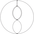
$R_{1}$

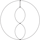
$R_{2}$

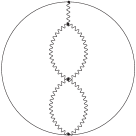
$R_{3}$

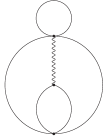
$R_{4}$

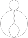
$R_{5}$

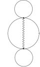
$R_{6}$

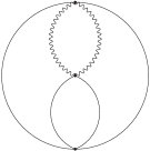
$M_{1}$

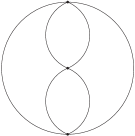
$M_{2}$

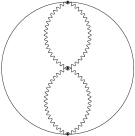
$M_{3}$

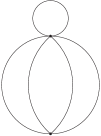
$M_{4}$

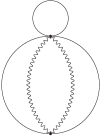
$M_{5}$

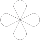
$M_{6}$

Figure 1: List of independent topologies belonging to the $n_{f}^{2}$-contribution. The topologies $R_{1}$-$R_{6}$ are reducible, whereas the topologies $M_{1}$-$M_{6}$ are master integrals. The wavy and solid lines depict massless and massive propagators respectively.

Through the expansion in the external momentum $q$ the derivatives acting on the polarization function generate additional powers of the denominators of the integrands. The deeper the expansion is, the higher powers are obtained. Let $M_{d}$ denote the sum of powers of propagators $D_{i}$ minus the number of propagators of the generic integral. Let $M_{p}$ denote the total sum of powers of the irreducible scalar products in the numerator of the integrand. Then one obtains integrands with $M_{d}$ up to $8$ and $M_{p}$ up to $3$, for an expansion of the $n_{f}^{2}$-contribution up to the first physical moment.

For the reduction of these integrals to a set of a few master integrals the standard method of IBP has been used. The reduction was implemented following the ideas described in ref. [10, 13, 14]. In order to reduce the polarization function to master integrals for an expansion up to the first physical moment a system of around 880000 equations has to be generated and solved. For a deeper expansion of the polarization function one obtains higher values for $M_{d}$ and $M_{p}$. This requires a huger system of IBP-identities in order to obtain a reduction to master integrals. A lexicographical ordering has been introduced assigning to each integral a weight describing its “complexity”. Integrals with increasing powers of the denominator and increasing number of irreducible scalar products are denoted as increasingly complicated. The linear system of equations has been solved with a program based on FORM3 [15] which uses FERMAT [16] for simplifying the rational functions in the space-time dimension $d$, which arise in this procedure. Complicated integrals are systematically expressed in terms of simpler ones and then substituted into the other equations. Some contributions have been checked independently with the program SOLVE [17] from which also some experience concerning the procedure of ordering the integrals according to their complexity has been gained. Masking of large integral coefficients is used, a strategy also adopted in the program AIR [18].

Exploiting the symmetries of the diagrams by reshuffling the powers of the propagators of a given topology in a unique way strongly reduces the size of the initial input and, similarly, in the second step the number of equations which need to be solved.

The solution of the system leads to a set of a around 130000 independent equations. With the help of these equations the first two Taylor coefficients of the polarization function can be expressed in terms of 6 master integrals $M_{1}$-$M_{6}$, with denominator powers one and no irreducible scalar products ($M_{d}=0,\,M_{p}=0$), which are shown in Fig. 1.

Calculation of the master integrals

The master integrals which belong to the diagrams $M_{1}-M_{6}$ are defined in $d=4-2\,\varepsilon$ space-time dimensions through

$$M_{1} = {\mu^{16-4\,d}\over N^{4}}\int{d^{d}\ell_{1}\over(2\,\pi)^{d}}\,{d^{d}\ell_{2}\over(2\,\pi)^{d}}\,{d^{d}\ell_{3}\over(2\,\pi)^{d}}\,{d^{d}\ell_{4}\over(2\,\pi)^{d}}\;{1\over D_{1}\,D_{2}\,D_{4}\,D_{7}\,D_{8}\,D_{10}},$$ (7)

$$M_{2} = {\mu^{16-4\,d}\over N^{4}}\int{d^{d}\ell_{1}\over(2\,\pi)^{d}}\,{d^{d}\ell_{2}\over(2\,\pi)^{d}}\,{d^{d}\ell_{3}\over(2\,\pi)^{d}}\,{d^{d}\ell_{4}\over(2\,\pi)^{d}}\;{1\over D_{1}\,D_{2}\,D_{3}\,D_{4}\,D_{9}\,D_{10}},$$ (8)

$$M_{3} = {\mu^{16-4\,d}\over N^{4}}\int{d^{d}\ell_{1}\over(2\,\pi)^{d}}\,{d^{d}\ell_{2}\over(2\,\pi)^{d}}\,{d^{d}\ell_{3}\over(2\,\pi)^{d}}\,{d^{d}\ell_{4}\over(2\,\pi)^{d}}\;{1\over D_{4}\,D_{5}\,D_{6}\,D_{7}\,D_{8}\,D_{10}},$$ (9)

$$M_{4} = {\mu^{16-4\,d}\over N^{4}}\int{d^{d}\ell_{1}\over(2\,\pi)^{d}}\,{d^{d}\ell_{2}\over(2\,\pi)^{d}}\,{d^{d}\ell_{3}\over(2\,\pi)^{d}}\,{d^{d}\ell_{4}\over(2\,\pi)^{d}}\;{1\over D_{1}\,D_{2}\,D_{3}\,D_{4}\,D_{9}},$$ (10)

$$M_{5} = {\mu^{16-4\,d}\over N^{4}}\int{d^{d}\ell_{1}\over(2\,\pi)^{d}}\,{d^{d}\ell_{2}\over(2\,\pi)^{d}}\,{d^{d}\ell_{3}\over(2\,\pi)^{d}}\,{d^{d}\ell_{4}\over(2\,\pi)^{d}}\;{1\over D_{2}\,D_{4}\,D_{5}\,D_{7}\,D_{9}},$$ (11)

$$M_{6} = {\mu^{16-4\,d}\over N^{4}}\int{d^{d}\ell_{1}\over(2\,\pi)^{d}}\,{d^{d}\ell_{2}\over(2\,\pi)^{d}}\,{d^{d}\ell_{3}\over(2\,\pi)^{d}}\,{d^{d}\ell_{4}\over(2\,\pi)^{d}}\;{1\over D_{1}\,D_{2}\,D_{3}\,D_{4}}$$ (12)

with

$$\begin{array}[]{l@{\quad}l@{\quad}l}D_{1}=\ell_{1}^{2}+m^{2}-i\,\epsilon,&D_{5}=\ell_{1}^{2}-i\,\epsilon,&D_{8}=(\ell_{1}+\ell_{2}+\ell_{3})^{2}-i\,\epsilon,\\ D_{2}=\ell_{2}^{2}+m^{2}-i\,\epsilon,&D_{6}=\ell_{2}^{2}-i\,\epsilon,&D_{9}=(\ell_{1}+\ell_{2}+\ell_{3})^{2}+m^{2}-i\,\epsilon,\\ D_{3}=\ell_{3}^{2}+m^{2}-i\,\epsilon,&D_{7}=\ell_{3}^{2}-i\,\epsilon,&D_{10}=(\ell_{1}+\ell_{2}+\ell_{4})^{2}+m^{2}-i\,\epsilon,\\ D_{4}=\ell_{4}^{2}+m^{2}-i\,\epsilon\end{array}$$ (13)

and the normalization factor

$$N=\varepsilon\,\mu^{4-d}\int{d^{d}\ell_{1}\over(2\,\pi)^{d}}{1\over D_{1}^{2}}={1\over 16\,\pi^{2}}\,\Gamma(1+\varepsilon)\,\left({m^{2}\over 4\,\pi\mu^{2}}\right)^{-\varepsilon}.$$ (14)

The factor $\mu$ denotes the renormalization scale.

Before calculating the master integral $M_{1}$ we consider at first the following combination of integrals with dots, where a dot on a line denotes an additional power of the associated denominator

$m^{2}$ $+\;\;{m^{2}\over\varepsilon}\;$ $=\;N_{10}+\mathcal{O}(\varepsilon)$.

(15)

The three-loop topology in the left hand side of eq. (15) as well as all following three-loop diagrams are normalized by $N^{3}$ (of eq. (14)). The combination in eq. (15) is finite and can be integrated numerically, with the result $N_{10}=5.3111546\dots$.

The relation between the dotted topologies in eq. (15) and master integrals can be obtained via IBP. One finds the following relations:

     $={(d-3)^{3}\,(2\,d-7)\over 16\,(d-4)\,m^{6}}$      $+\;{(d-3)\,(d-2)\,(3\,d-8)\,(7\,d^{2}-48\,d+82)\over 128\,(d-4)\,(2\,d-7)\,m^{8}}$      ,

(16)

     $=-{3\,(d-3)\,(3\,d-10)\,(3\,d-8)\over 256\,(d-4)\,m^{6}}$  $-\;{(d-2)^{2}\,(11\,d-38)\over 128\,(d-4)\,m^{8}}$      .

(17)

The three-loop integrals in the right hand side of eq. (17) and the factorizable four-loop amplitude in the right hand side of eq. (16) can be calculated with MATAD [8] or taken from ref. [19]. Inserting eq. (16) and (17) into eq. (15) leads to

$$M_{1} = m^{4}\,\bigg{(}{2\over 3\,\varepsilon^{4}}+{4\over\varepsilon^{3}}+{38\over 3\,\varepsilon^{2}}+{4\over 3\,\varepsilon}\,\left(11+4\,\zeta_{3}\right)-{2\over 15}\,\left(885+2\,\pi^{4}-660\,\zeta_{3}\right)$$ (18)

$$- {4\,\varepsilon\over 15}\,(4335-1440\,a_{4}-60\,\log^{4}({2})+120\,N_{10}+60\,\log^{2}({2})\,\pi^{2}$$

$$+ 23\,\pi^{4}-2690\,\zeta_{3}-360\,\zeta_{5})+\mathcal{O}(\varepsilon^{2})\bigg{)},$$

with

$$\hfill\zeta_{n}=\sum_{k=1}^{\infty}\,{1\over k^{n}}\hskip 8.5359pt\mbox{and}\hskip 8.5359pta_{4}=\sum_{k=1}^{\infty}{1\over 2^{k}k^{4}}.$$ (19)

The same procedure has been applied for calculating the master integral $M_{2}$. The topology $M_{2}$ with 3 symmetrical distributed dots is finite

$m^{2}\,$ $=N_{20}+\mathcal{O}(\varepsilon)$

(20)

and can be integrated numerically. The calculation yields $N_{20}=5.40925606\dots$. The master integral $M_{2}$ can be calculated using the IBP identity
$=-\;{(d-4)\,(d-3)^{3}\,(2\,d-7)\over 6\,(3\,d-13)\,(3\,d-11)\,m^{6}}$     $-\;{(d-3)\,(d-2)\,(3\,d-8)\,(13\,d^{2}-99\,d+182)\over 512\,(3\,d-13)\,(3\,d-11)\,m^{8}}$                  $+\;{(d-2)^{4}\,(d-1)\over 256\,(3\,d-13)\,(3\,d-11)\,m^{10}}$      ,

(21)

inserting eq. (21) into eq. (20) and solving with respect to $M_{2}$ results in:

$$M_{2} = m^{4}\,\bigg{(}{3\over 2\,\varepsilon^{4}}+{19\over 2\,\varepsilon^{3}}+{67\over 2\,\varepsilon^{2}}+{1\over 2\,\varepsilon}\,\left(127-6\,N_{20}+21\,\zeta_{3}\right)+\mathcal{O}(\varepsilon^{0})\bigg{)}.$$

This result is in agreement with eq. (4) in ref. [21].
The calculation of the master integral $M_{3}$ is easy,

$$M_{3} = m^{4}\,\bigg{(}{1\over 6\,\varepsilon^{4}}+{5\over 6\,\varepsilon^{3}}+{3\over 2\,\varepsilon^{2}}-{1\over 6\,\varepsilon}\,(39-38\,\zeta_{3})-{1\over 60}\,(4710+23\,\pi^{4}$$ (22)

$$- 1900\,\zeta_{3})-{\varepsilon\over 12}\,\left(5934+23\,\pi^{4}-684\,\zeta_{3}-2580\,\zeta_{5}\right)+\mathcal{O}(\varepsilon^{2})\bigg{)}.$$

For completeness we also give the results for the factorized master integrals

$$M_{4} = m^{6}\,\bigg{(}-{2\over\varepsilon^{4}}-{29\over 3\,\varepsilon^{3}}-{163\over 6\,\varepsilon^{2}}-{601\over 12\,\varepsilon}-{1\over 24}\,\left(635+896\,\zeta_{3}\right)+{\varepsilon\over 720}\,(204705$$

$$- 184320\,a_{4}-7680\,\log^{4}({2})+7680\,\log^{2}({2})\,\pi^{2}+2176\,\pi^{4}-228480\,\zeta_{3})+\mathcal{O}(\varepsilon^{2})\bigg{)},$$

$$M_{5} = m^{6}\,\bigg{(}-{1\over 3\,\varepsilon^{4}}-{3\over 2\,\varepsilon^{3}}-{43\over 12\,\varepsilon^{2}}-{1\over 24\,\varepsilon}\,\left(81+64\,\zeta_{3}\right)+{1\over 240}\,(3985+32\,\pi^{4}$$

$$- 2880\,\zeta_{3})+{\varepsilon\over 480}\,\left(60435+288\,\pi^{4}-13760\,\zeta_{3}-23040\,\zeta_{5}\right)+\mathcal{O}(\varepsilon^{2})\bigg{)},$$

$$M_{6} = m^{8}\,\left({1\over\varepsilon^{4}}+{4\over\varepsilon^{3}}+{10\over\varepsilon^{2}}+{20\over\varepsilon}+35+56\,\varepsilon+\mathcal{O}(\varepsilon^{2})\right).$$

Result for the $\mathcal{O}(\alpha_{s}^{3}n_{f}^{2})$ contribution

Inserting the above master integrals into the reduced $n_{f}^{2}$-contribution and performing renormalization of the strong coupling constant $\alpha_{s}$, the external current and the mass $m=\overline{m}(\mu^{2})$ in the $\overline{\mbox{MS}}$-scheme, leads to the following result for the first two moments of the four-loop $\mathcal{O}(\alpha_{s}^{3}n_{f}^{2})$ contribution of the heavy quark vacuum polarization function:

$$\hat{C}^{(3)}_{0} = n_{l}\,n_{h}\,\Bigg{(}{7043\over 11664}-{127\over 108}\,\zeta_{3}+{1\over 6}\,N_{10}+\left({37\over 324}-{7\over 24}\,\zeta_{3}\right)\,l_{\mu}+{2\over 27}\,l_{\mu}^{2}-{2\over 27}\,l_{\mu}^{3}\Bigg{)}$$

$$+ n_{h}^{2}\,\Bigg{(}{610843\over 816480}+{1439\over 540}\,\zeta_{3}-{157\over 210}\,N_{20}+\left({113\over 324}-{7\over 24}\,\zeta_{3}\right)\,l_{\mu}+{1\over 27}\,l_{\mu}^{2}-{1\over 27}\,l_{\mu}^{3}\Bigg{)}$$

$$+ n_{l}^{2}\,\Bigg{(}{17897\over 23328}-{31\over 54}\,\zeta_{3}-{19\over 81}\,l_{\mu}+{1\over 27}\,l_{\mu}^{2}-{1\over 27}\,l_{\mu}^{3}\Bigg{)}$$

and (23)

$$\hat{C}^{(3)}_{1} = n_{l}\,n_{h}\,\Bigg{(}{262877\over 262440}-{38909\over 19440}\,\zeta_{3}+{29\over 81}\,N_{10}$$ (24)

$$\qquad+\left({3779\over 21870}-{203\over 324}\,\zeta_{3}\right)\,l_{\mu}+{472\over 3645}\,l_{\mu}^{2}-{16\over 135}\,l_{\mu}^{3}\Bigg{)}$$

$$+ n_{h}^{2}\,\Bigg{(}{163868\over 98415}+{13657\over 2430}\,\zeta_{3}-{5648\over 3645}\,N_{20}$$

$$\qquad+\left({14483\over 21870}-{203\over 324}\,\zeta_{3}\right)\,l_{\mu}+{236\over 3645}\,l_{\mu}^{2}-{8\over 135}\,l_{\mu}^{3}\Bigg{)}$$

$$+ n_{l}^{2}\,\Bigg{(}{42173\over 32805}-{112\over 135}\,\zeta_{3}-{1784\over 3645}\,l_{\mu}+{236\over 3645}\,l_{\mu}^{2}-{8\over 135}\,l_{\mu}^{3}\Bigg{)}$$

with $l_{\mu}=\log\left({\mu^{2}\over m^{2}}\right)$.
The $n_{l}^{2}$-contribution has been checked independently by taking into account the corresponding two-loop case, in which the gluon propagator has been replaced by a gluon propagator containing a renormalon chain with two massless fermion one-loop insertions. The computation has been performed in a general $\xi$-gauge and it has been checked that the dependence on the gauge parameter vanishes. Furthermore it has been checked that both coefficient functions $C_{0}$ and $C_{1}$ meet the standard renormalization group equation. Numerically one finds for the coefficient $C_{0}$ and $C_{1}$ at $\mu=m$:

$$C_{0} = a_{s}\,1.4444+a_{s}^{2}\,\left(1.5863+0.1387\,n_{h}+0.3714\,n_{l}\right)$$

$$+ a_{s}^{3}\,\left(0.0252\,n_{h}\,n_{l}+0.0257\,n_{l}^{2}-0.0309\,n_{h}^{2}\right),$$

$$C_{1} = 1.0667+a_{s}\,2.5547+a_{s}^{2}\,\left(0.2461+0.2637\,n_{h}+0.6623\,n_{l}\right)$$

$$+ a_{s}^{3}\,\left(0.1658\,n_{h}\,n_{l}+0.0961\,n_{l}^{2}+0.0130\,n_{h}^{2}\right).$$

4 Summary and Conclusion

Using the IBP method and Laporta’s algorithm, we have evaluated a gauge invariant subset of the four-loop tadpole amplitudes contributing to derivatives of the vacuum polarization at $q^{2}=0$. All loop integrals have been mapped on a minimal set of independent topologies. Then an elaborate automated procedure has been developed and applied, which identifies equivalent amplitudes, factorizable contributions, discards massless tadpoles, and performs symmetrization. Solving a system of nearly one million linear equations, all amplitudes can be expressed through six master integrals. These have been evaluated analytically or numerically to high precision. The present work can be seen as a first step towards the evaluation of the full set of four-loop amplitude contributions to the vacuum polarization function.

Acknowledgments:
We would like to thank Mikhail Tentyukov for generous support and a lot of advice in our dealing with FORM and FERMAT. Furthermore we thank Matthias Steinhauser for careful reading the manuscript and advice. We are grateful to Michael Faisst for discussions. C.S. would like to thank the Graduiertenkolleg “Hochenergiephysik und Teilchenastrophysik” for financial support. The work of P.M. was partially supported by the Marie Curie Training Site “Particle Physics at Present and Future Colliders”. This work was supported by the SFB/TR 9 (Computational Particle Physics).

References

• [1] K. G. Chetyrkin, J. H. KΓΌhn and A. Kwiatkowski, Phys. Rep. 277 (1996) 189.
• [2] M. Steinhauser, Phys. Rept. 364 (2002) 247.
• [3] K. G. Chetyrkin, J. H. KΓΌhn and M. Steinhauser, Nucl. Phys. B482 (1996) 213.
• [4] K. G. Chetyrkin, R. Harlander and M. Steinhauser, Phys. Rev. D58 (1998) 014012.
• [5] K. G. Chetyrkin, J. H. KΓΌhn and M. Steinhauser , Nucl. Phys. B505 (1997) 40.
• [6] J. H. KΓΌhn and M. Steinhauser, Nucl. Phys. B619 (2001) 588.
• [7] D. J. Broadhurst , Z. Phys. C54 (1992) 599.
• [8] M. Steinhauser, Comput. Phys. Commun. 134 (2001) 335.
• [9] K. G. Chetyrkin and F. V. Tkachov, Nucl. Phys. B192 (1981) 159.
• [10] S. Laporta, Int. J. Mod. Phys. A15 (2000) 5087.
• [11] T. van Ritbergen, J. A. M. Vermaseren and S. A. Larin, Phys. Lett. B400, (1997) 379.
• [12] M. Czakon, The four-loop QCD beta-function and anomalous dimensions, (2004), hep-ph/0411261.
• [13] Y. SchrΓΆder, Nucl. Phys. Proc. Suppl. 116 (2003) 402.
• [14] P. Mastrolia, and E. Remiddi , Nucl. Phys. Proc. Suppl. 89 (2000) 76.
• [15] J. A. M. Vermaseren, New features of FORM, (2000), math-ph/0010025.
• [16] R. H. Lewis, Fermat’s User Guide, http://www.bway.net/~lewis/.
• [17] E. Remiddi, SOLVE, unpublished, available from the author.
• [18] C. Anastasiou and A. Lazopoulos , JHEP 07 (2004) 046.
• [19] S. Laporta and E. Remiddi, Acta Phys. Polon. B28 (1997) 959.
• [20] Y. SchrΓΆder and M. Steinhauser, private communication,
Y. SchrΓΆder and A. Vuorinen,
in preparation.
• [21] S. Laporta, Phys. Lett. B549 (2002) 115.