Dark Matter Candidates in Supersymmetric Models¹

hep-ph/0412054

UMN–TH–2332/04

FTPI–MINN–04/45

December 2004

The status of the constrained minimal supersymmetric standard model (CMSSM) will be discussed in light of our current understanding of the relic density after WMAP. A global likelihood analysis of the model is performed including data from direct Higgs searches, global fits to electroweak data, $b\to s\gamma$, the anomalous magnetic moment of the muon, as well as the cosmological relic density. Also considered are models which relax and further constrain the CMSSM. Prospects for dark matter detection in colliders and cryogenic detectors will be briefly discussed.

1 Introduction

Supersymmetric models with conserved $R$-parity contain one new stable particle which is a candidate for cold dark matter (CDM) EHNOS . There are very strong constraints, however, forbidding the existence of stable or long lived particles which are not color and electrically neutral. The sneutrino snu is one possible candidate, but in the MSSM, it has been excluded as a dark matter candidate by direct dir and indirect indir searches. Another possibility is the gravitino and is probably the most difficult to exclude. This possibility has been discussed recently in the CMSSM context gdm . I will concentrate on the remaining possibility in the MSSM, namely the neutralinos.

There are four neutralinos, each of which is a linear combination of the $R=-1$, neutral fermions EHNOS : the wino $\tilde{W}^{3}$, the partner of the 3rd component of the $SU(2)_{L}$ gauge boson; the bino, $\tilde{B}$, the partner of the $U(1)_{Y}$ gauge boson; and the two neutral Higgsinos, $\tilde{H}_{1}$ and $\tilde{H}_{2}$. In general, the neutralino mass eigenstates can be expressed as a linear combination

$$\chi=\alpha\tilde{B}+\beta\tilde{W}^{3}+\gamma\tilde{H}_{1}+\delta\tilde{H}_{2}$$ (1)

The solution for the coefficients $\alpha,\beta,\gamma$ and $\delta$ for neutralinos that make up the LSP can be found by diagonalizing the mass matrix which depends on $M_{1}(M_{2})$ which are the soft supersymmetry breaking U(1) (SU(2)) gaugino mass terms, $\mu$, the supersymmetric Higgs mixing mass parameter and the two Higgs vacuum expectation values, $v_{1}$ and $v_{2}$. One combination of these is related to the $Z$ mass, and therefore is not a free parameter, while the other combination, the ratio of the two vevs, $\tan\beta$, is free.

The most general version of the MSSM, despite its minimality in particles and interactions contains well over a hundred new parameters. The study of such a model would be untenable were it not for some (well motivated) assumptions. These have to do with the parameters associated with supersymmetry breaking. It is often assumed that, at some unification scale, all of the gaugino masses receive a common mass, $m_{1/2}$. The gaugino masses at the weak scale are determined by running a set of renormalization group equations. Similarly, one often assumes that all scalars receive a common mass, $m_{0}$, at the GUT scale. These too are run down to the weak scale. The remaining supersymmetry breaking parameters are the trilinear mass terms, $A_{0}$, which I will also assume are unified at the GUT scale, and the bilinear mass term $B$. There are, in addition, two physical CP violating phases which will not be considered here.

The natural boundary conditions at the GUT scale for the MSSM would include $\mu$ and $B$ in addition to $m_{1/2}$, $m_{0}$, and $A_{0}$. In this case, upon running the RGEs down to a low energy scale and minimizing the Higgs potential, one would predict the values of $M_{Z}$, $\tan\beta$ (in addition to all of the sparticle masses). Since $M_{Z}$ is known, it is more useful to analyze supersymmetric models where $M_{Z}$ is input rather than output. It is also common to treat $\tan\beta$ as an input parameter. This can be done at the expense of shifting $\mu$ (up to a sign) and $B$ from inputs to outputs. This model is often referred to as the constrained MSSM or CMSSM. Once these parameters are set, the entire spectrum of sparticle masses at the weak scale can be calculated. In the CMSSM, the solutions for $\mu$ generally lead to a neutralino which which very nearly a pure $\tilde{B}$.

2 The CMSSM after WMAP

For a given value of $\tan\beta$, $A_{0}$, and $sgn(\mu)$, the resulting regions of acceptable relic density and which satisfy the phenomenological constraints can be displayed on the $m_{1/2}-m_{0}$ plane. In Fig. 1a, the light shaded region corresponds to that portion of the CMSSM plane with $\tan\beta=10$, $A_{0}=0$, and $\mu>0$ such that the computed relic density yields $0.1<\Omega_{\chi}h^{2}<0.3$. At relatively low values of $m_{1/2}$ and $m_{0}$, there is a large ‘bulk’ region which tapers off as $m_{1\!/2}$ is increased. At higher values of $m_{0}$, annihilation cross sections are too small to maintain an acceptable relic density and $\Omega_{\chi}h^{2}>0.3$. Although sfermion masses are also enhanced at large $m_{1\!/2}$ (due to RGE running), co-annihilation processes between the LSP and the next lightest sparticle (in this case the ${\widetilde{\tau}}_{\scriptscriptstyle\rm 1}$) enhance the annihilation cross section and reduce the relic density. This occurs when the LSP and NLSP are nearly degenerate in mass. The dark shaded region has $m_{{\widetilde{\tau}}_{\scriptscriptstyle\rm 1}}<m_{\chi}$ and is excluded. Neglecting coannihilations, one would find an upper bound of $\sim 450{\rm\,Ge\kern-1.25ptV}$ on $m_{1\!/2}$, corresponding to an upper bound of roughly $200{\rm\,Ge\kern-1.25ptV}$ on $m_{\tilde{B}}$. The effect of coannihilations is to create an allowed band about 25-50 ${\rm\,Ge\kern-1.25ptV}$ wide in $m_{0}$ for $m_{1\!/2}\mathrel{\raise 1.29167pt\hbox{$<$\kern-7.5pt\lower 4.30554pt\hbox{$\sim$}}}1400{\rm\,Ge\kern-1.25ptV}$, which tracks above the $m_{\tilde{\tau}_{1}}=m_{\chi}$ contour efo .

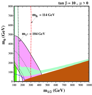
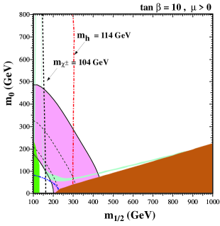
Figure 1: The $(m_{1/2},m_{0})$ planes for (a) $\tan\beta=10$ and $\mu>0$, assuming $A_{0}=0,m_{t}=175$ GeV and $m_{b}(m_{b})^{\overline{MS}}_{SM}=4.25$ GeV. The near-vertical (red) dot-dashed lines are the contours $m_{h}=114$ GeV, and the near-vertical (black) dashed line is the contour $m_{\chi^{\pm}}=104$ GeV. Also shown by the dot-dashed curve in the lower left is the corner excluded by the LEP bound of $m_{\tilde{e}}>99$ GeV. The medium (dark green) shaded region is excluded by $b\to s\gamma$, and the light (turquoise) shaded area is the cosmologically preferred regions with $0.1\leq\Omega_{\chi}h^{2}\leq 0.3$. In the dark (brick red) shaded region, the LSP is the charged ${\tilde{\tau}}_{1}$. The region allowed by the E821 measurement of $a_{\mu}$ at the 2-$\sigma$ level, is shaded (pink) and bounded by solid black lines, with dashed lines indicating the 1-$\sigma$ ranges. In (b), the relic density is restricted to the range $0.094<\Omega_{\chi}h^{2}<0.129$.

Also shown in Fig. 1a are the relevant phenomenological constraints. These include the limit on the chargino mass: $m_{\chi^{\pm}}>104$ GeV LEPsusy , on the selectron mass: $m_{\tilde{e}}>99$ GeV LEPSUSYWG_0101 and on the Higgs mass: $m_{h}>114$ GeV LEPHiggs . The former two constrain $m_{1/2}$ and $m_{0}$ directly via the sparticle masses, and the latter indirectly via the sensitivity of radiative corrections to the Higgs mass to the sparticle masses, principally $m_{\tilde{t},\tilde{b}}$. FeynHiggs FeynHiggs is used for the calculation of $m_{h}$. The Higgs limit imposes important constraints principally on $m_{1/2}$ particularly at low $\tan\beta$. Another constraint is the requirement that the branching ratio for $b\rightarrow s\gamma$ is consistent with the experimental measurements bsgex . These measurements agree with the Standard Model, and therefore provide bounds on MSSM particles gam ; bsgth , such as the chargino and charged Higgs masses, in particular. Typically, the $b\rightarrow s\gamma$ constraint is more important for $\mu<0$, but it is also relevant for $\mu>0$, particularly when $\tan\beta$ is large. The constraint imposed by measurements of $b\rightarrow s\gamma$ also excludes small values of $m_{1/2}$. Finally, there are regions of the $(m_{1/2},m_{0})$ plane that are favoured by the BNL measurement newBNL of $g_{\mu}-2$ at the 2-$\sigma$ level, corresponding to a deviation from the Standard Model calculation Davier using $e^{+}e^{-}$ data. One should be however aware that this constraint is still under active discussion.

The preferred range of the relic LSP density has been altered significantly by the recent improved determination of the allowable range of the cold dark matter density obtained by combining WMAP and other cosmological data: $0.094<\Omega_{CDM}<0.129$ at the 2-$\sigma$ level WMAP . In the second panel of Fig. 1, we see the effect of imposing the WMAP range on the neutralino density eoss ; Baer ; morewmap . We see immediately that (i) the cosmological regions are generally much narrower, and (ii) the ‘bulk’ regions at small $m_{1/2}$ and $m_{0}$ have almost disappeared, in particular when the laboratory constraints are imposed. Looking more closely at the coannihilation regions, we see that (iii) they are significantly truncated as well as becoming much narrower, since the reduced upper bound on $\Omega_{\chi}h^{2}$ moves the tip where $m_{\chi}=m_{\tilde{\tau}}$ to smaller $m_{1/2}$ so that the upper limit is now $m_{1/2}\mathrel{\raise 1.29167pt\hbox{$<$\kern-7.5pt\lower 4.30554pt\hbox{$\sim$}}}950$ GeV or $m_{\chi}\mathrel{\raise 1.29167pt\hbox{$<$\kern-7.5pt\lower 4.30554pt\hbox{$\sim$}}}400$ GeV.

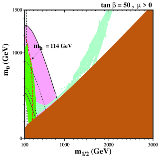
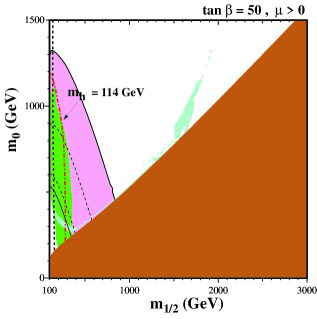
Figure 2: As in Fig. 1 for $\tan\beta=50$.

Another mechanism for extending the allowed CMSSM region to large $m_{\chi}$ is rapid annihilation via a direct-channel pole when $m_{\chi}\sim{1\over 2}m_{A}$ funnel ; EFGOSi . Since the heavy scalar and pseudoscalar Higgs masses decrease as $\tan\beta$ increases, eventually $2m_{\chi}\simeq m_{A}$ yielding a ‘funnel’ extending to large $m_{1/2}$ and $m_{0}$ at large $\tan\beta$, as seen in the high $\tan\beta$ strips of Fig. 2. As one can see, the impact of the Higgs mass constraint is reduced (relative to the case with $\tan\beta=10$) while that of $b\to s\gamma$ is enhanced.

Shown in Fig. 3 are the WMAP lines eoss of the $(m_{1/2},m_{0})$ plane allowed by the new cosmological constraint $0.094<\Omega_{\chi}h^{2}<0.129$ and the laboratory constraints listed above, for $\mu>0$ and values of $\tan\beta$ from 5 to 55, in steps $\Delta(\tan\beta)=5$. We notice immediately that the strips are considerably narrower than the spacing between them, though any intermediate point in the $(m_{1/2},m_{0})$ plane would be compatible with some intermediate value of $\tan\beta$. The right (left) ends of the strips correspond to the maximal (minimal) allowed values of $m_{1/2}$ and hence $m_{\chi}$. The lower bounds on $m_{1/2}$ are due to the Higgs mass constraint for $\tan\beta\leq 23$, but are determined by the $b\to s\gamma$ constraint for higher values of $\tan\beta$.

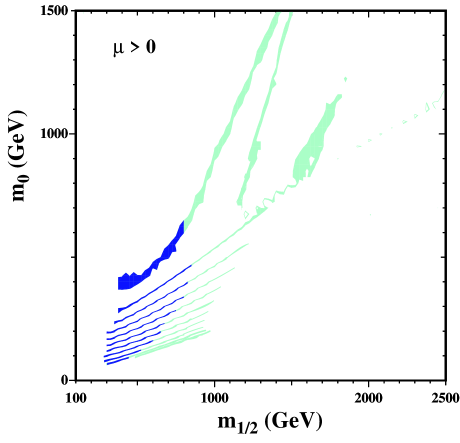
Figure 3: The strips display the regions of the $(m_{1/2},m_{0})$ plane that are compatible with $0.094<\Omega_{\chi}h^{2}<0.129$ and the laboratory constraints for $\mu>0$ and $\tan\beta=5,10,15,20,25,30,35,40,45,50,55$. The parts of the strips compatible with $g_{\mu}-2$ at the 2-$\sigma$ level have darker shading.

Finally, there is one additional region of acceptable relic density known as the focus-point region fp , which is found at very high values of $m_{0}$. An example showing this region is found in Fig. 4, plotted for $\tan\beta=10$, $\mu>0$, and $m_{t}=175$ TeV. As $m_{0}$ is increased, the solution for $\mu$ at low energies as determined by the electroweak symmetry breaking conditions eventually begins to drop. When $\mu\mathrel{\raise 1.29167pt\hbox{$<$\kern-7.5pt\lower 4.30554pt\hbox{$\sim$}}}m_{1/2}$, the composition of the LSP gains a strong Higgsino component and as such the relic density begins to drop precipitously. These effects are both shown in Fig. 5 where the value of $\mu$ and $\Omega h^{2}$ are plotted as a function of $m_{0}$ for fixed $m_{1/2}=300$ GeV and $\tan\beta=10$. As $m_{0}$ is increased further, there are no longer any solutions for $\mu$. This occurs in the shaded region in the upper left corner of Fig. 4.

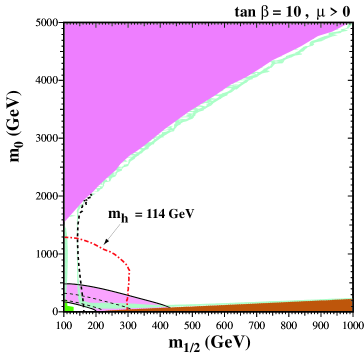
Figure 4: As in Fig. 1a, where the range in $m_{0}$ is extended to 5 TeV. In the shaded region at very high $m_{0}$, there are no solutions for $\mu$ which respect the low energy electroweak symmetry breaking conditions.

Fig. 5 also exemplifies the degree of fine tuning associated with the focus-point region. While the position of the focus-point region in the $m_{0},m_{1/2}$ plane is not overly sensitive to supersymmetric parameters, it is highly sensitive to the top quark Yukawa coupling which contributes to the evolution of $\mu$ rs ; ftuning . As one can see in the figure, a change in $m_{t}$ of 3 GeV produces a shift of about 2.5 TeV in $m_{0}$. Note that the position of the focus-point region is also highly sensitive to the value of $A_{0}/m_{0}$. In Fig. 5, $A_{0}=0$ was chosen. For $A_{0}/m_{0}=0.5$, the focus point shifts from 2.5 to 4.5 TeV and moves to larger $m_{0}$ as $A_{0}/m_{0}$ is increased.

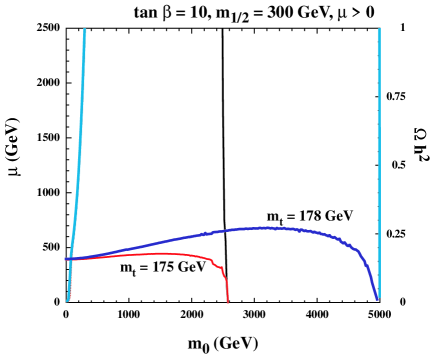
Figure 5: The value of $\mu$ as a function of $m_{0}$ for fixed $m_{1/2}=300$ GeV and $\tan\beta=10$ for two choices of $m_{t}$ as indicated. The scale on the right gives the value of $\Omega h^{2}$. The curves corresponding to this is scale rise sharply at low $m_{0}$ to values much larger than 1. For $m_{t}=175$ GeV and $m_{0}\approx 2500$ GeV, the value of $\Omega h^{2}$ drops to acceptable values when $\mu$ becomes small. When the $m_{t}=178$ GeV, $\Omega h^{2}$ drops at $m_{0}\approx 5000$ GeV.

3 A Likelihood analysis of the CMSSM

Up to now, in displaying acceptable regions of cosmological density in the $m_{0},m_{1/2}$ plane, it has been assumed that the input parameters are known with perfect accuracy so that the relic density can be calculated precisely. While all of the beyond the standard model parameters are completely unknown and therefore carry no formal uncertainties, standard model parameters such as the top and bottom Yukawa couplings are known but do carry significant uncertainties. Indeed, we saw that in the case of the focus-point region, there is an intense sensitivity of the relic density to the top quark Yukawa. Other regions in the $m_{0},m_{1/2}$ plane, such as those corresponding to the rapid annihilation funnels are also very sensitive to the 3rd generation Yukawas.

The optimal way to combine the various constraints (both phenomenological and cosmological) is via a likelihood analysis, as has been done by some authors both before DeBoer and after Baer the WMAP data was released. When performing such an analysis, in addition to the formal experimental errors, it is also essential to take into account theoretical errors, which introduce systematic uncertainties that are frequently non-negligible. Recently, we have preformed an extensive likelihood analysis of the CMSSM eoss4 . Included is the full likelihood function for the LEP Higgs search, as released by the LEP Higgs Working Group. This includes the small enhancement in the likelihood just beyond the formal limit due to the LEP Higgs signal reported late in 2000. This was re-evaluated most recently in LEPHiggs , and cannot be regarded as significant evidence for a light Higgs boson. We have also taken into account the indirect information on $m_{h}$ provided by a global fit to the precision electroweak data. The likelihood function from this indirect source does not vary rapidly over the range of Higgs masses found in the CMSSM, but we included this contribution with the aim of completeness.

The interpretation of the combined Higgs likelihood, ${\cal L}_{exp}$, in the $(m_{1/2},m_{0})$ plane depends on uncertainties in the theoretical calculation of $m_{h}$. These include the experimental error in $m_{t}$ and (particularly at large $\tan\beta$) $m_{b}$, and theoretical uncertainties associated with higher-order corrections to $m_{h}$. Our default assumptions are that $m_{t}=175\pm 5$ GeV for the pole mass, and $m_{b}=4.25\pm 0.25$ GeV for the running $\overline{MS}$ mass evaluated at $m_{b}$ itself. The theoretical uncertainty in $m_{h}$, $\sigma_{th}$, is dominated by the experimental uncertainties in $m_{t,b}$, which are treated as uncorrelated Gaussian errors:

$$\sigma_{th}^{2}=\left(\frac{\partial m_{h}}{\partial m_{t}}\right)^{2}\Delta m_{t}^{2}+\left(\frac{\partial m_{h}}{\partial m_{b}}\right)^{2}\Delta m_{b}^{2}\,.$$ (2)

Typically, we find that $(\partial m_{h}/\partial m_{t})\sim 0.5$, so that $\sigma_{th}$ is roughly 2-3 GeV.

The combined experimental likelihood, ${\cal L}_{exp}$, from direct searches at LEP 2 and a global electroweak fit is then convolved with a theoretical likelihood (taken as a Gaussian) with uncertainty given by $\sigma_{th}$ from (2) above. Thus, we define the total Higgs likelihood function, ${\cal L}_{h}$, as

$${\cal L}_{h}(m_{h})={{\cal N}\over{\sqrt{2\pi}\,\sigma_{th}}}\int dm^{\prime}_{h}\,\,{\cal L}_{exp}(m^{\prime}_{h})\,\,e^{-(m^{\prime}_{h}-m_{h})^{2}/2\sigma_{th}^{2}}\,,$$ (3)

where ${\cal N}$ is a factor that normalizes the experimental likelihood distribution.

In addition to the Higgs likelihood function, we have included the likelihood function based on $b\to s\gamma$. The branching ratio for these decays has been measured by the CLEO, BELLE and BaBar collaborations bsgex , and we took as the combined value ${\cal{B}}(b\to s\gamma)=(3.54\pm 0.41\pm 0.26)\times 10^{-4}$. The theoretical prediction gam ; bsgth contains uncertainties which stem from the uncertainties in $m_{b}$, $\alpha_{s}$, the measurement of the semileptonic branching ratio of the $B$ meson as well as the effect of the scale dependence. While the likelihood function based on the measurements of the anomalous magnetic moment of the muon was considered in eoss4 , it will not be discussed here.

Finally, in calculating the likelihood of the CDM density, we take into account the contribution of the uncertainties in $m_{t,b}$. We will see that the theoretical uncertainty plays a very significant role in this analysis. The likelihood for $\Omega h^{2}$ is therefore,

$${\cal L}_{\Omega h^{2}}=\frac{1}{\sqrt{2\pi}\sigma}e^{-({\Omega h^{2}}^{th}-{\Omega h^{2}}^{exp})^{2}/2\sigma^{2}}\,,$$ (4)

where $\sigma^{2}=\sigma_{exp}^{2}+\sigma_{th}^{2}$, with $\sigma_{exp}$ taken from the WMAP WMAP result and $\sigma_{th}^{2}$ from (2), replacing $m_{h}$ by $\Omega h^{2}$.

The total likelihood function is computed by combining all the components described above:

$${\cal L}_{tot}={\cal L}_{h}\times{\cal L}_{bs\gamma}\times{\cal L}_{\Omega_{\chi}h^{2}}(\times{\cal L}_{a_{\mu}})$$ (5)

The likelihood function in the CMSSM can be considered a function of two variables, ${\cal L}_{tot}(m_{1/2},m_{0})$, where $m_{1/2}$ and $m_{0}$ are the unified GUT-scale gaugino and scalar masses respectively. Results are based on a Bayesian analysis, in which a prior range for $m_{1/2}$ is introduced in order to normalize the conditional probability obtained from the likelihood function using Bayes’ theorem. Although it is possible to motivate some upper limit on $m_{1/2}$, e.g., on the basis of naturalness nat ; ftuning ; eos2 , one cannot quantify any such limit rigorously. Within the selected range, we adopt a flat prior distribution for $m_{1/2}$, and normalize the volume integral:

$$\int{\cal L}_{tot}\,dm_{0}\,dm_{1/2}\;=\;1$$ (6)

for each value of $\tan\beta$, combining where appropriate both signs of $\mu$. We note that no such prior need be specified for $m_{0}$. For any given value of $m_{1/2}$, the theory is well defined only up to some maximum value of $m_{0}$, above which radiative electroweak symmetry breaking is no longer possible. We always integrate up to that point, adopting also a flat prior distribution for $m_{0}$.

In Fig. 6 the likelihood along slices through the CMSSM parameter space for $\tan\beta=10,A_{0}=0,\mu>0,$ and $m_{1/2}=300$ and 800 GeV is shown in the left and right panels, respectively, plotting the likelihood as a function of $m_{0}$. The solid red curves show the total likelihood function calculated including the uncertainties which stem from the experimental errors in $m_{t}$ and $m_{b}$. The peak at low $m_{0}$ is due to the coannihilation region. The peak at $m_{0}\simeq 2500(4500)$ GeV for $m_{1/2}=300(800)$ GeV is due to the focus-point region. Also shown in Fig. 6 are the 68%, 90%, and 95% CL (horizontal) lines, corresponding to the iso-likelihood values of the fully integrated likelihood function corresponding to the solid (red) curve.

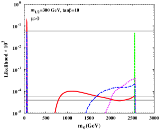
Figure 6: The likelihood function along slices in $m_{0}$ through the CMSSM parameter space for $\tan\beta=10,A_{0}=0,\mu>0$ and $m_{1/2}=300,800$ GeV in the left and right panels, respectively. The red (solid) curves are calculated using the current errors in $m_{t}$ and $m_{b}$, the green dashed curve with no error in $m_{t}$, the violet dotted lines with $\Delta m_{t}=0.5$ GeV, and the blue dashed-dotted lines with $\Delta m_{t}=1$ GeV.

The focus-point peak is suppressed relative to the coannihilation peak at low $m_{0}$ because of the theoretical sensitivity to the experimental uncertainty in the top mass. We recall that the likelihood function is proportional to $\sigma^{-1}$, and that $\sigma$ which scales with $\partial(\Omega_{\chi}h^{2})/\partial m_{t}$, is very large at large $m_{0}$ ftuning . The error due to the uncertainty in $m_{t}$ is far greater in the focus-point region than in the coannihilation region. Thus, even though the exponential in ${\cal L}_{\Omega_{\chi}h^{2}}$ is of order unity near the focus-point region when $\Omega_{\chi}h^{2}\simeq 0.1$, the prefactor is very small due the large uncertainty in the top mass. This accounts for the factor of $\mathrel{\raise 1.29167pt\hbox{$>$\kern-7.5pt\lower 4.30554pt\hbox{$\sim$}}}1000$ suppression seen in Fig. 6 when comparing the two peaks of the solid red curves.

We note also that there is another broad, low-lying peak at intermediate values of $m_{0}$. This is due to a combination of the effects of $\sigma$ in the prefactor and the exponential. We expect a bump to occur when the Gaussian exponential is of order unity, i.e., $\Omega_{\chi}h^{2}\sim\sqrt{2}\Delta m_{t}\,\partial\Omega_{\chi}h^{2}/\partial m_{t}$. $\Omega_{\chi}h^{2}\sim 10$ at large $m_{0}$ for our nominal value $m_{t}$ = 175 GeV, but it varies significantly as one samples the favoured range of $m_{t}$ within its present uncertainty. The competition between the exponential and the prefactor would require a large theoretical uncertainty in $\Omega_{\chi}h^{2}$: $\partial\Omega_{\chi}h^{2}/\partial m_{t}\sim 2$ for $\Delta m_{t}=5$ GeV. This occurs when $m_{0}\sim 1000$ GeV, which is the position of the broad secondary peak in Fig. 6a. At higher $m_{0}$, $\sigma$ continues to grow, and the prefactor suppresses the likelihood function until $\Omega_{\chi}h^{2}$ drops to $\sim 0.1$ in the focus-point region.

As is clear from the above discussion, the impact of the present experimental error in $m_{t}$ is particularly important in this region. This point is further demonstrated by the differences between the curves in each panel, where we decrease ad hoc the experimental uncertainty in $m_{t}$. As $\Delta m_{t}$ is decreased, the intermediate bump blends into the broad focus-point peak. When the uncertainties in $m_{t}$ and $m_{b}$ are set to 0, we obtain a narrow peak in the focus-point region.

Using the fully normalized likelihood function ${\cal L}_{tot}$ obtained by combining both signs of $\mu$ for each value of $\tan\beta$, we can determine the regions in the $(m_{1/2},m_{0})$ planes which correspond to specific CLs. Fig. 7 extends the previous analysis to the entire $(m_{1/2},m_{0})$ plane for $\tan\beta=10$ and $A_{0}=0$, including both signs of $\mu$. The darkest (blue), intermediate (red) and lightest (green) shaded regions are, respectively, those where the likelihood is above 68%, above 90%, and above 95%. Overall, the likelihood for $\mu<0$ is less than that for $\mu>0$ due to the Higgs and $b\to s\gamma$ constraints. Only the bulk and coannihilation-tail regions appear above the 68% level, but the focus-point region appears above the 90% level, and so cannot be excluded.

Figure 7: Contours of the likelihood at the 68%, 90% and 95% levels for $\tan\beta=10$, $A_{0}=0$ and $\mu>0$ (left panel) or $\mu<0$ (right panel), calculated using information of $m_{h}$, $b\to s\gamma$ and $\Omega_{CDM}h^{2}$ and the current uncertainties in $m_{t}$ and $m_{b}$.

The bulk region is more apparent in the right panel of Fig. 7 for $\mu>0$ than it would be if the experimental error in $m_{t}$ and the theoretical error in $m_{h}$ were neglected. Fig. 8 complements the previous figures by showing the likelihood functions as they would appear if there were no uncertainty in $m_{t}$, keeping the other inputs the same. We see that, in this case, both the coannihilation and focus-point strips rise above the 68% CL.

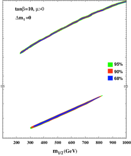
Figure 8: As in Fig. 7 but assuming zero uncertainty in $m_{t}$.

Fig. 9 shows the likelihood projection for $\tan\beta=50$, $A_{0}=0$ and $\mu>0$. In this case, regions at small $m_{1/2}$ and $m_{0}$ are disfavoured by the $b\to s\gamma$ constraint. The coannihilation region is broadened by a merger with the rapid-annihilation funnel. Both the coannihilation and the focus-point regions feature strips allowed at the 68% CL, and these are linked by a bridge at the 95% CL.

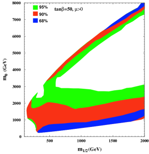
Figure 9: Likelihood contours as in Fig. 7, but for $\tan\beta=50$, $A_{0}=0$ and $\mu>0$.

4 Beyond the CMSSM

The results of the CMSSM described in the previous sections are based heavily on the assumptions of universality of the supersymmetry breaking parameters. One of the simplest generalizations of this model relaxes the assumption of universality of the Higgs soft masses and is known as the NUHM eos3 In this case, the input parameters include $\mu$ and $m_{A},$ in addition to the standard CMSSM inputs. In order to switch $\mu$ and $m_{A}$ from outputs to inputs, the two soft Higgs masses, $m_{1},m_{2}$ can no longer be set equal to $m_{0}$ and instead are calculated from the electroweak symmetry breaking conditions. The NUHM parameter space was recently analyzed eos3 and a sample of the results are shown in Fig. 10.

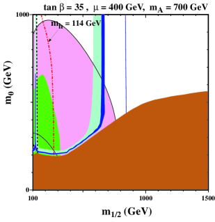
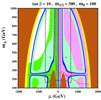
Figure 10: a) The NUHM $(m_{1/2},m_{0})$ plane for $\tan\beta=35$, (a) $\mu=400$ GeV and $m_{A}=700$ GeV b)the NUHM $(\mu,m_{A})$ plane for $\tan\beta=10$, $m_{0}=100$ GeV and $m_{1/2}=300$ GeV, with $A_{0}=0$. The (red) dot-dashed lines are the contours $m_{h}=114$ GeV, and the near-vertical (black) dashed lines are the contours $m_{\chi^{\pm}}=103.5$ GeV. The dark (black) dot-dashed lines indicate the GUT stability constraint. Only the areas inside these curves (small $\mu$) are allowed by this constraint. The light (turquoise) shaded areas are the cosmologically preferred regions with $0.1\leq\Omega_{\chi}h^{2}\leq 0.3$. The darker (blue) portion of this region corresponds to the newer WMAP densities. The dark (brick red) shaded regions is excluded because a charged particle is lighter than the neutralino, and the lighter (yellow) shaded regions is excluded because the LSP is a sneutrino. The medium (green) shaded region is excluded by $b\to s\gamma$. The regions allowed by the $g-2$ constraint are shaded (pink) and bounded by solid black lines. The solid (blue) curves correspond to $m_{\chi}=m_{A}/2$.

In the left panel of Fig. 10, we see a $m_{1/2},m_{0}$ plane with a relative low value of $\mu$. In this case, an allowed region is found when the LSP contains a non-negligible Higgsino component which moderates the relic density independent of $m_{0}$. To the right of this region, the relic density is too small. In the right panel, we see an example of the $m_{A},\mu$ plane. The crosses correspond to CMSSM points. In this single pane, we see examples of acceptable cosmological regions corresponding to the bulk region, co-annihilation region and s-channel annihilation through the Higgs pseudo scalar.

Rather than relax the CMSSM, it is in fact possible to further constrain the model. While the CMSSM models described above are certainly mSUGRA inspired, minimal supergravity models can be argued to be still more predictive. Let us assume that supersymmetry is broken in a hidden sector so that the superpotential can be written as a sum of two terms, $W=F(\phi)+g(\zeta)$, where $\phi$ represents all observable fields and $\zeta$ all hidden sector fields. We furthermore must choose $g(\zeta)$ such that when $\zeta$ picks up a vacuum expectation value, supersymmetry is broken. When the potential is expanded and terms inversely proportional to Planck mass are dropped, one finds BIM 1) scalar mass universality with $m_{0}=\langle g\rangle$; 2) trilinear mass universality with $A_{0}=\langle dg/d\zeta\rangle\langle\zeta\rangle+\langle g\rangle\langle\zeta\rangle^{2}$; and 3) $B_{0}=A_{0}-m_{0}$.

In the simplest version of the theory pol , the universal trilinear soft supersymmetry-breaking terms are $A=(3-\sqrt{3})m_{0}$ and bilinear soft supersymmetry-breaking term is $B=(2-\sqrt{3})m_{0}$, i.e., a special case of the general relation above between $B$ and $A$.

Given a relation between $B_{0}$ and $A_{0}$, we can no longer use the standard CMSSM boundary conditions, in which $m_{1/2}$, $m_{0}$, $A_{0}$, $\tan\beta$, and $sgn(\mu)$ are input at the GUT scale with $\mu$ and $B$ determined by the electroweak symmetry breaking condition. Now, one is forced to input $B_{0}$ and instead $\tan\beta$ is calculated from the minimization of the Higgs potential eoss2 .

In Fig. 11, the contours of $\tan\beta$ (solid blue lines) in the $(m_{1/2},m_{0})$ planes for two values of ${\hat{A}}=A_{0}/m_{0}$, ${\hat{B}}=B_{0}/m_{0}={\hat{A}}-1$ and the sign of $\mu$ are displayed eoss2 . Also shown are the contours where $m_{\chi^{\pm}}>104$ GeV (near-vertical black dashed lines) and $m_{h}>114$ GeV (diagonal red dash-dotted lines). The excluded regions where $m_{\chi}>m_{\tilde{\tau}_{1}}$ have dark (red) shading, those excluded by $b\to s\gamma$ have medium (green) shading, and those where the relic density of neutralinos lies within the WMAP range $0.094\leq\Omega_{\chi}h^{2}\leq 0.129$ have light (turquoise) shading. Finally, the regions favoured by $g_{\mu}-2$ at the 2-$\sigma$ level are medium (pink) shaded.

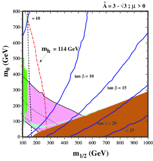
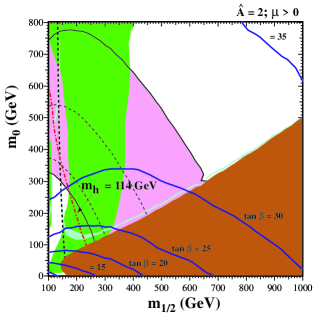
Figure 11: Examples of $(m_{1/2},m_{0})$ planes with contours of $\tan\beta$ superposed, for $\mu>0$ and (a) the simplest Polonyi model with ${\hat{A}}=3-\sqrt{3},{\hat{B}}={\hat{A}}-1$ and (b) ${\hat{A}}=2.0,{\hat{B}}={\hat{A}}-1$. In each panel, we show the regions excluded by the LEP lower limits on MSSM particles, those ruled out by $b\to s\gamma$ decay (medium green shading), and those excluded because the LSP would be charged (dark red shading). The region favoured by the WMAP range has light turquoise shading. The region suggested by $g_{\mu}-2$ is medium (pink) shaded.

In panel (a) of Fig. 11, we see that the Higgs constraint combined with the relic density requires $\tan\beta\mathrel{\raise 1.29167pt\hbox{$>$\kern-7.5pt\lower 4.30554pt\hbox{$\sim$}}}11$, whilst the relic density also enforces $\tan\beta\mathrel{\raise 1.29167pt\hbox{$<$\kern-7.5pt\lower 4.30554pt\hbox{$\sim$}}}20$. For a given point in the $m_{1/2}-m_{0}$ plane, the calculated value of $\tan\beta$ increases as ${\hat{A}}$ increases. This is seen in panel (b) of Fig. 11, when ${\hat{A}}=2.0$, close to its maximal value for $\mu>0$, the $\tan\beta$ contours turn over towards smaller $m_{1/2}$, and only relatively large values $25\mathrel{\raise 1.29167pt\hbox{$<$\kern-7.5pt\lower 4.30554pt\hbox{$\sim$}}}\tan\beta\mathrel{\raise 1.29167pt\hbox{$<$\kern-7.5pt\lower 4.30554pt\hbox{$\sim$}}}35$ are allowed by the $b\to s\gamma$ and $\Omega_{CDM}h^{2}$ constraints, respectively. For any given value of ${\hat{A}}$, there is only a relatively narrow range allowed for $\tan\beta$.

5 Detectability

The question of detectability with respect to supersymmetric models is of key importance particularly with the approaching start of the LHC. As an aid to the assessment of the prospects for detecting sparticles at different accelerators, benchmark sets of supersymmetric parameters have often been found useful, since they provide a focus for concentrated discussion oldbench ; SPS ; newbench . A set of proposed post-LEP benchmark scenarios oldbench were chosen to span the CMSSM. Five of the chosen points are in the ‘bulk’ region at small $m_{1/2}$ and $m_{0}$, four are spread along the coannihilation ‘tail’ at larger $m_{1/2}$ for various values of $\tan\beta$. Two points are in rapid-annihilation ‘funnels’ at large $m_{1/2}$ and $m_{0}$. Two points were chosen in the focus-point region at large $m_{0}$. The proposed points range over the allowed values of $\tan\beta$ between 5 and 50.

In Fig. 12, a comparison of the numbers of different MSSM particles that should be observable at different accelerators in the various benchmark scenarios newbench , ordered by their consistency with $g_{\mu}-2$. The qualities of the prospective sparticle observations at hadron colliders and linear $e^{+}e^{-}$ colliders are often very different, with the latters’ clean experimental environments providing prospects for measurements with better precision. Nevertheless, Fig. 12 already restates the clear message that hadron colliders and linear $e^{+}e^{-}$ colliders are largely complementary in the classes of particles that they can see, with the former offering good prospects for strongly-interacting sparticles such as squarks and gluinos, and the latter excelling for weakly-interacting sparticles such as charginos, neutralinos and sleptons.

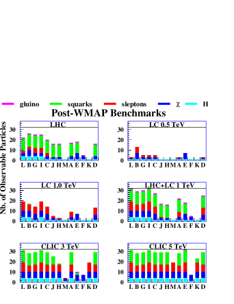
Figure 12: Summary of the numbers of MSSM particles that may be detectable at various accelerators in the updated benchmark scenarios. We see that the capabilities of the LHC and of linear $e^{+}e^{-}$ colliders are largely complementary. We re-emphasize that mass and coupling measurements at $e^{+}e^{-}$ colliders are usually much cleaner and more precise than at hadron-hadron colliders such as the LHC, where, for example, it is not known how to distinguish the light squark flavours.

Clearly the center of mass energy of any future linear collider is paramount towards the supersymmetry discovery potential of the machine. This is seen in Fig. 12 for the benchmark points as more sparticles become observable at higher CM energy. We can emphasize this point in general models by plotting the masses of the two lightest (observable) sparticles in supersymmetric models. For example, in Fig. 13 eoss7 , a scatter plot of the masses of the lightest visible supersymmetric particle (LVSP) and the next-to-lightest visible supersymmetric particle (NLVSP) is shown for the CMSSM. Once again, points selected satisfy all phenomenological constraints. We do not consider the LSP itself to be visible, nor any heavier neutral sparticle that decays invisibly inside the detector, such as ${\tilde{\nu}}\to\nu\chi$ when ${\tilde{\nu}}$ is the next-to-lightest sparticle in a neutralino LSP scenario. The LVSP and the NLVSP are the lightest sparticles likely to be observable in collider experiments.

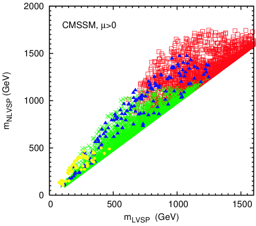
Figure 13: Scatter plots of the masses of the lightest visible supersymmetric particle (LVSP) and the next-to-lightest visible supersymmetric particle (NLVSP) in the CMSSM for $\mu>0$. The darker (blue) triangles satisfy all the laboratory, astrophysical and cosmological constraints. For comparison, the dark (red) squares and medium-shaded (green) crosses respect the laboratory constraints, but not those imposed by astrophysics and cosmology. In addition, the (green) crosses represent models which are expected to be visible at the LHC. The very light (yellow) points are those for which direct detection of supersymmetric dark matter might be possible.

All points shown in Fig. 13 satisfy the phenomenological constraints discussed above. The dark (red) squares represent those points for which the relic density is outside the WMAP range, and for which all coloured sparticles (squarks and gluinos) are heavier than 2 TeV. The CMSSM parameter reach at the LHC has been analyzed in Baer2 . To within a few percent accuracy, the CMSSM reach contours presented in Baer2 coincide with the 2-TeV contour for the lightest squark (generally the stop) or gluino, so we regard the dark (red) points as unobservable at the LHC. Most of these points have $m_{NLVSP}\mathrel{\raise 1.29167pt\hbox{$>$\kern-7.5pt\lower 4.30554pt\hbox{$\sim$}}}1.2$ TeV. Conversely, the medium-shaded (green) crosses represent points where at least one squark or gluino has a mass less than 2 TeV and should be observable at the LHC. The spread of the dark (red) squares and medium-shaded (green) crosses, by as much as 500 GeV or more in some cases, reflects the maximum mass splitting between the LVSP and the NLVSP that is induced in the CMSSM via renormalization effects on the input mass parameters. The amount of this spread also reflects our cutoff $|A_{0}|<1$ TeV, which controls the mass splitting of the third generation sfermions.

The darker (blue) triangles are those points respecting the cosmological cold dark matter constraint. Comparing with the regions populated by dark (red) squares and medium-shaded (green) crosses, one can see which of these models would be detectable at the LHC, according to the criterion in the previous paragraph. We see immediately that the dark matter constraint restricts the LVSP masses to be less than about 1250 GeV and NLVSP masses to be less than about 1500 GeV. In most cases, the identity of the LVSP is the lighter $\tilde{\tau}$. While pair-production of the LVSP would sometimes require a CM energy of about 2.5 TeV, in some cases there is a lower supersymmetric threshold due to the associated production of the LSP $\chi$ with the next lightest neutralino $\chi_{2}$ djou . Examining the masses and identities of the sparticle spectrum at these points, we find that $E_{CM}\mathrel{\raise 1.29167pt\hbox{$>$\kern-7.5pt\lower 4.30554pt\hbox{$\sim$}}}2.2$ TeV would be sufficient to see at least one sparticle, as shown in Table 1. Similarly, only a LC with $E_{CM}\geq 2.5$ TeV would be ‘guaranteed’ to see two visible sparticles (in addition to the $\chi$ LSP), somewhat lower than the 3.0 TeV one might obtain by requiring the pair production of the NLVSP. Points with $m_{LVSP}\mathrel{\raise 1.29167pt\hbox{$>$\kern-7.5pt\lower 4.30554pt\hbox{$\sim$}}}700$ GeV are predominantly due to rapid annihilation via direct-channel $H,A$ poles, while points with 200 GeV $\mathrel{\raise 1.29167pt\hbox{$<$\kern-7.5pt\lower 4.30554pt\hbox{$\sim$}}}m_{LVSP}\mathrel{\raise 1.29167pt\hbox{$<$\kern-7.5pt\lower 4.30554pt\hbox{$\sim$}}}$ 700 GeV are largely due to $\chi$-slepton coannihilation.

Table 1: Centre-of-mass energy (in TeV) required to observe one or two sparticles at a future LC in the CMSSM and NUHM.

Model	$sgn(\mu)$	one sparticle	two sparticles
CMSSM	$\mu>0$	2.2	2.6
	$\mu<0$	2.2	2.5
NUHM	$\mu>0$	2.4	2.8
	$\mu<0$	2.6	2.9

An $E_{CM}=500$ GeV LC would be able to explore the ‘bulk’ region at low $(m_{1/2},m_{0})$, which is represented by the small cluster of points around $m_{LVSP}\sim 200$ GeV. It should also be noted that there are a few points with $m_{LVSP}\sim 100$ GeV which are due to rapid annihilation via the light Higgs pole. These points all have very large values of $m_{0}$ which relaxes the Higgs mass and chargino mass constraints, particularly when $m_{t}=178$ GeV. A LC with $E_{CM}=1000$ GeV would be able to reach some way into the coannihilation ‘tail’, but would not cover all the WMAP-compatible dark (blue) triangles. Indeed, about a third of these points are even beyond the reach of the LHC in this model. Finally, the light (yellow) filled circles are points for which the elastic $\chi$-$p$ scattering cross section is larger than $10^{-8}$ pb.

Because the LSP as dark matter is present locally, there are many avenues for pursuing dark matter detection. Direct detection techniques rely on an ample neutralino-nucleon scattering cross-section. The prospects for direct detection for the benchmark points discussed above EFFMO are shown in Fig. 14. This figure shows rates for the elastic spin-independent and spin dependent scattering cross sections of supersymmetric relics on protons. Indirect searches for supersymmetric dark matter via the products of annihilations in the galactic halo or inside the Sun also have prospects in some of the benchmark scenarios EFFMO .

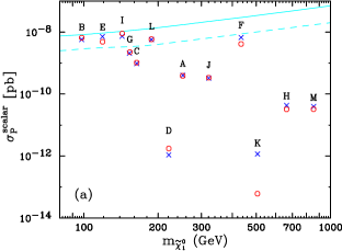
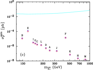
Figure 14: Elastic cross sections for (a) spin-independent scattering and (b) spin-dependent scattering on protons. Our predictions (blue crosses) are compared with those of Neutdriver Neutdriver (red circles) for neutralino-nucleon scattering. Projected sensitivities (a) for CDMS II Schnee:1998gf and CRESST Bravin:1999fc (solid) and GENIUS GENIUS (dashed) and (b) for a 100 kg NAIAD array Spooner:2000kt are also shown.

In Fig. 15, we display the allowed ranges of the spin-independent cross sections in the NUHM when we sample randomly $\tan\beta$ as well as the other NUHM parameters efloso . The raggedness of the boundaries of the shaded regions reflects the finite sample size. The dark shaded regions includes all sample points after the constraints discussed above (including the relic density constraint) have been applied. In a random sample, one often hits points which are are perfectly acceptable at low energy scales but when the parameters are run to high energies approaching the GUT scale, one or several of the sparticles mass squared runs negative fors . This has been referred to as the GUT constraint here. The medium shaded region embodies those points after the GUT constraint has been applied. After incorporating all the cuts, including that motivated by $g_{\mu}-2$, we find that the light shaded region where the scalar cross section has the range $10^{-6}$ pb $\mathrel{\raise 1.29167pt\hbox{$>$\kern-7.5pt\lower 4.30554pt\hbox{$\sim$}}}\sigma_{SI}\mathrel{\raise 1.29167pt\hbox{$>$\kern-7.5pt\lower 4.30554pt\hbox{$\sim$}}}10^{-10}$ pb, with somewhat larger (smaller) values being possible in exceptional cases. If the $g_{\mu}-2$ cut is removed, the upper limits on the cross sections are unchanged, but much lower values become possible: $\sigma_{SI}\ll 10^{-13}$ pb. The effect of the GUT constraint on more general supersymmetric models was discussed in eoss3 .

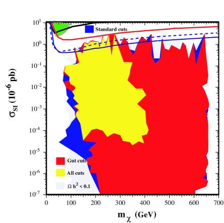
Figure 15: Ranges of the spin-independent cross section in the NUHM. The ranges allowed by the cuts on $\Omega_{\chi}h^{2}$, $m_{h}$ and $b\to s\gamma$ have dark shading, those still allowed by the GUT stability cut have medium shading, and those still allowed after applying all the cuts including $g_{\mu}-2$ have light shading. The pale shaded region corresponds to the extra area of points with low relic densities, whose cross sections have been rescaled appropriately. Also shown are the limits from the CDMScdms and Edelweissedel experiments as well as the recent CDMSII result cdms2 on the neutralino-proton elastic scattering cross section as a function of the neutralino mass. The CDMSII limit is stronger than the Edelweiss limit which is stronger than the previous CDMS limit at higher $m_{\chi}$. The result reported by DAMA dama is found in the upper left.

The results from this analysis efloso for the scattering cross section in the NUHM (which by definition includes all CMSSM results) are compared with the previous CDMS cdms and Edelweiss edel bounds as well as the recent CDMSII results cdms2 in Fig. 15. While previous experimental sensitivities were not strong enough to probe predictions of the NUHM, the current CDMSII bound has begun to exclude realistic models and it is expected that these bounds improve by a factor of about 20.

This work was partially supported by DOE grant DE-FG02-94ER-40823.

References

- (1) H. Goldberg, Phys. Rev. Lett. 50, 1419 (1983); J. Ellis, J.S. Hagelin, D.V. Nanopoulos, K.A. Olive and M. Srednicki, Nucl. Phys. B238, 453 (1984).
- (2) L.E. Ibanez, Phys. Lett. 137B, 160 (1984); J. Hagelin, G.L. Kane, and S. Raby, Nucl., Phys. B241, 638 (1984); T. Falk, K. A. Olive and M. Srednicki, Phys. Lett. B 339, 248 (1994).
-
(3)
S. Ahlen, et. al., Phys. Lett. B195, 603 (1987);
D.D. Caldwell, et. al., Phys. Rev. Lett. 61, 510 (1988);
M. Beck et al., Phys. Lett. B336 141 (1994). -
(4)
see e.g. K.A. Olive and M. Srednicki,
Phys. Lett. 205B, 553 (1988);
N. Sato et al. Phys.Rev. D44, 2220 (1991). - (5) J. Ellis, T. Falk, and K.A. Olive, Phys.Lett. B444 (1998) 367 [arXiv:hep-ph/9810360]; J. Ellis, T. Falk, K.A. Olive, and M. Srednicki, Astr. Part. Phys. 13 (2000) 181 [Erratum-ibid. 15 (2001) 413] [arXiv:hep-ph/9905481].
- (6) J. L. Feng, S. Su and F. Takayama, arXiv:hep-ph/0404231; arXiv:hep-ph/0404198; J. L. Feng, A. Rajaraman and F. Takayama, Phys. Rev. Lett. 91 (2003) 011302 [arXiv:hep-ph/0302215]; J. R. Ellis, K. A. Olive, Y. Santoso and V. C. Spanos, Phys. Lett. B 588 (2004) 7 [arXiv:hep-ph/0312262]; L. Roszkowski and R. Ruiz de Austri, arXiv:hep-ph/0408227.
-
(7)
Joint LEP 2 Supersymmetry Working Group,
Combined LEP Chargino Results, up to 208 GeV,
http://lepsusy.web.cern.ch/lepsusy/www/inos_moriond01/charginos_pub.html. -
(8)
Joint LEP 2 Supersymmetry Working Group, Combined LEP
Selectron/Smuon/Stau Results, 183-208 GeV,
http://lepsusy.web.cern.ch/lepsusy/www/sleptons_summer02/slep_2002.html. -
(9)
LEP Higgs Working Group for Higgs boson searches, OPAL Collaboration,
ALEPH Collaboration, DELPHI Collaboration and L3
Collaboration,
Phys. Lett. B 565 (2003) 61 [arXiv:hep-ex/0306033].
Searches for the neutral Higgs bosons of the MSSM: Preliminary
combined results using LEP data collected at energies up to 209 GeV,
LHWG-NOTE-2001-04, ALEPH-2001-057, DELPHI-2001-114, L3-NOTE-2700,
OPAL-TN-699, arXiv:hep-ex/0107030; LHWG Note/2002-01,
http://lephiggs.web.cern.ch/LEPHIGGS/papers/July2002_SM/index.html. - (10) S. Heinemeyer, W. Hollik and G. Weiglein, Comput. Phys. Commun. 124 (2000) 76 [arXiv:hep-ph/9812320]; S. Heinemeyer, W. Hollik and G. Weiglein, Eur. Phys. J. C 9 (1999) 343 [arXiv:hep-ph/9812472].
- (11) S. Chen et al. [CLEO Collaboration], Phys. Rev. Lett. 87 (2001) 251807 [arXiv:hep-ex/0108032]; BELLE Collaboration, BELLE-CONF-0135. See also K. Abe et al. [Belle Collaboration], Phys. Lett. B 511 (2001) 151 [arXiv:hep-ex/0103042]; B. Aubert et al. [BaBar Collaboration], arXiv:hep-ex/0207076.
- (12) C. Degrassi, P. Gambino and G. F. Giudice, JHEP 0012 (2000) 009 [arXiv:hep-ph/0009337], as implemented by P. Gambino and G. Ganis.
- (13) M. Carena, D. Garcia, U. Nierste and C. E. Wagner, Phys. Lett. B 499 (2001) 141 [arXiv:hep-ph/0010003]; P. Gambino and M. Misiak, Nucl. Phys. B 611 (2001) 338; D. A. Demir and K. A. Olive, Phys. Rev. D 65 (2002) 034007 [arXiv:hep-ph/0107329]; T. Hurth, arXiv:hep-ph/0106050; Rev. Mod. Phys. 75, 1159 (2003) [arXiv:hep-ph/0212304].
- (14) [The Muon g-2 Collaboration], Phys. Rev. Lett. 92 (2004) 161802, hep-ex/0401008.
- (15) M. Davier, S. Eidelman, A. Höcker and Z. Zhang, Eur. Phys. J. C 31 (2003) 503, hep-ph/0308213; see also K. Hagiwara, A. Martin, D. Nomura and T. Teubner, Phys. Rev. D 69 (2004) 093003, hep-ph/0312250; S. Ghozzi and F. Jegerlehner, Phys. Lett. B 583 (2004) 222, hep-ph/0310181; M. Knecht, hep-ph/0307239; K. Melnikov and A. Vainshtein, hep-ph/0312226; J. de Troconiz and F. Yndurain, hep-ph/0402285.
- (16) C. L. Bennett et al., Astrophys. J. Suppl. 148 (2003) 1; D. N. Spergel et al., Astrophys. J. Suppl. 148 (2003) 175; H. V. Peiris et al., Astrophys. J. Suppl. 148 (2003) 213.
- (17) J. R. Ellis, K. A. Olive, Y. Santoso and V. C. Spanos, Phys. Lett. B 565 (2003) 176 [arXiv:hep-ph/0303043].
- (18) H. Baer and C. Balazs, JCAP 0305 (2003) 006 [arXiv:hep-ph/0303114].
- (19) A. B. Lahanas and D. V. Nanopoulos, Phys. Lett. B 568 (2003) 55 [arXiv:hep-ph/0303130]; U. Chattopadhyay, A. Corsetti and P. Nath, Phys. Rev. D 68 (2003) 035005 [arXiv:hep-ph/0303201]; C. Munoz, Int. J. Mod. Phys. A 19, 3093 (2004) [arXiv:hep-ph/0309346] R. Arnowitt, B. Dutta and B. Hu, arXiv:hep-ph/0310103.
- (20) M. Drees and M. M. Nojiri, Phys. Rev. D47 (1993) 376; H. Baer and M. Brhlik, Phys. Rev. D53 (1996) 59; and Phys. Rev. D57 (1998) 567; H. Baer, M. Brhlik, M. A. Diaz, J. Ferrandis, P. Mercadante, P. Quintana and X. Tata, Phys. Rev. D63 (2001) 015007; A. B. Lahanas, D. V. Nanopoulos and V. C. Spanos, Mod. Phys. Lett. A16 (2001) 1229.
- (21) J. R. Ellis, T. Falk, G. Ganis, K. A. Olive and M. Srednicki, Phys. Lett. B510 (2001) 236 [arXiv:hep-ph/0102098].
- (22) J. L. Feng, K. T. Matchev and T. Moroi, Phys. Rev. D 61 (2000) 075005 [arXiv:hep-ph/9909334].
- (23) A. Romanino and A. Strumia, Phys. Lett. B 487 (2000) 165, hep-ph/9912301.
- (24) J. R. Ellis and K. A. Olive, Phys. Lett. B 514 (2001) 114 [arXiv:hep-ph/0105004].
- (25) W. de Boer, M. Huber, C. Sander and D. I. Kazakov, arXiv:hep-ph/0106311.
- (26) J. R. Ellis, K. A. Olive, Y. Santoso and V. C. Spanos, Phys. Rev. D 69 (2004) 095004 [arXiv:hep-ph/0310356].
- (27) J. R. Ellis, K. Enqvist, D. V. Nanopoulos and F. Zwirner, Mod. Phys. Lett. A 1 (1986) 57; R. Barbieri and G. F. Giudice, Nucl. Phys. B 306 (1988) 63.
- (28) J. R. Ellis, K. A. Olive and Y. Santoso, New J. Phys. 4 (2002) 32 [arXiv:hep-ph/0202110].
- (29) J. Ellis, K. Olive and Y. Santoso, Phys.Lett. B539 (2002) 107 [arXiv:hep-ph/0204192].; J. R. Ellis, T. Falk, K. A. Olive and Y. Santoso, Nucl. Phys. B 652 (2003) 259 [arXiv:hep-ph/0210205].
- (30) For reviews, see: H. P. Nilles, Phys. Rep. 110 (1984) 1; A. Brignole, L. E. Ibanez and C. Munoz, arXiv:hep-ph/9707209, published in Perspectives on supersymmetry, ed. G. L. Kane, pp. 125-148; H.-P. Nilles, M. Srednicki and D. Wyler, Phys. Lett. 120B (1983) 345; L.J. Hall, J. Lykken and S. Weinberg, Phys. Rev. D27 (1983) 2359.
- (31) J. Polonyi, Budapest preprint KFKI-1977-93 (1977); R. Barbieri, S. Ferrara and C.A. Savoy, Phys. Lett. 119B (1982) 343.
- (32) J. R. Ellis, K. A. Olive, Y. Santoso and V. C. Spanos, Phys. Lett. B 573 (2003) 162 [arXiv:hep-ph/0305212]; Phys. Rev. D 70 (2004) 055005 [arXiv:hep-ph/0405110].
- (33) M. Battaglia et al., Eur. Phys. J. C 22 (2001) 535, hep-ph/0106204.
- (34) B. Allanach et al., Eur. Phys. J. C 25 (2002) 113, hep-ph/0202233.
- (35) M. Battaglia, A. De Roeck, J. Ellis, F. Gianotti, K. Olive and L. Pape, Eur. Phys. J. C 33 (2004) 273, hep-ph/0306219.
- (36) J. R. Ellis, K. A. Olive, Y. Santoso and V. C. Spanos, arXiv:hep-ph/0408118.
- (37) H. Baer, C. Balazs, A. Belyaev, T. Krupovnickas and X. Tata, JHEP 0306 (2003) 054 [arXiv:hep-ph/0304303].
- (38) A. Djouadi, M. Drees and J. L. Kneur, JHEP 0108 (2001) 055 [arXiv:hep-ph/0107316].
- (39) J. Ellis, J. L. Feng, A. Ferstl, K. T. Matchev and K. A. Olive, Eur. Phys. J. C24 (2002) 311 [arXiv:astro-ph/0110225].
- (40) G. Jungman, M. Kamionkowski and K. Griest, Phys. Rept. 267, 195 (1996) [arXiv:hep-ph/9506380]; http://t8web.lanl.gov/people/jungman/neut-package.html.
- (41) CDMS Collaboration, R. W. Schnee et al., Phys. Rep. 307 (1998) 283.
- (42) CRESST Collaboration, M. Bravin et al., Astropart. Phys. 12 (1999) 107.
- (43) H. V. Klapdor-Kleingrothaus, arXiv:hep-ph/0104028.
- (44) N. J. Spooner et al., Phys. Lett. B 473, 330 (2000).
- (45) J. R. Ellis, A. Ferstl, K. A. Olive and Y. Santoso, Phys. Rev. D 67, 123502 (2003) [arXiv:hep-ph/0302032].
- (46) T. Falk, K. A. Olive, L. Roszkowski and M. Srednicki, Phys. Lett. B 367 (1996) 183 [arXiv:hep-ph/9510308]; A. Riotto and E. Roulet, Phys. Lett. B 377 (1996) 60 [arXiv:hep-ph/9512401]; A. Kusenko, P. Langacker and G. Segre, Phys. Rev. D 54 (1996) 5824 [arXiv:hep-ph/9602414]; T. Falk, K. A. Olive, L. Roszkowski, A. Singh and M. Srednicki, Phys. Lett. B 396 (1997) 50 [arXiv:hep-ph/9611325].
- (47) J. R. Ellis, K. A. Olive, Y. Santoso and V. C. Spanos, Phys. Rev. D 69, 015005 (2004) [arXiv:hep-ph/0308075].
- (48) D. Abrams et al. [CDMS Collaboration], Phys.Rev. D66 (2002) 122003 [arXiv:astro-ph/0203500].
- (49) A. Benoit et al., Phys.Lett. B545 (2002) 43 [arXiv:astro-ph/0206271].
- (50) D. S. Akerib et al. [CDMS Collaboration], arXiv:astro-ph/0405033.
- (51) DAMA Collaboration, R. Bernabei et al., Phys. Lett. B436 (1998) 379.