An Integrated Tool for Loop Calculations: aITALC

Abstract

aITALC, a new tool for automating loop calculations in high energy physics, is described. The package creates Fortran code for two-fermion scattering processes automatically, starting from the generation and analysis of the Feynman graphs. We describe the modules of the tool, the intercommunication between them and illustrate its use with three examples.

DESY 04-226
SFB/CPP-04-63
hep-ph/0412047
December 2004

1 Program summary

• Title of the program: aITALC version 1.0 (29 October 2004)

• Catalogue identifier:

• Program obtainable from: http://www-zeuthen.desy.de/theory/aitalc

• Computer: PC i686

• Operating system: GNU/Linux, tested on different distributions SuSE 8.2 and 9.1, Red Hat 7.2, Debian 3.0. Also on Solaris

• Programming language used: GNU Make, Diana, Form, Fortran77

• Memory required to execute with typical data: Up to about 10 MB

• No. of processors used: 1

• No. of bytes in distributed program, including test data, etc.: 369516 bytes, including tutorial in postscript format

• Distribution format: tar gzip file

• High-speed storage required: from 1.5 to 30 MB, depending on modules present and unfolding of examples

• No. of cards in combined program and test deck:

• Keywords: Radiative corrections, automatic calculation, Feynman diagram, computer algebra, aITALC, Diana

• Nature of the physical problem: Calculation of differential cross sections for $e^{+}e^{-}$ annhilation in one-loop approximation.

• Method of solution: Generation and perturbative analysis of Feynman diagrams with later evaluation of matrix elements and form factors.

• Restriction of the complexity of the problem: The limit of application is, for the moment, the $2\to 2$ particles reactions in the electroweak standard model.

• Typical running time: Few minutes, being highly depending on the complexity of the process and the Fortran compiler.

2 Introduction

aITALC is designed as a tool to perform automated perturbative higher order calculations of cross sections in high energy physics.

The main goal is to create numerical programs directly from Feynman rules. It is actually developed for few known models like the electro-weak standard model (EWSM) and quantum electro-dynamic (QED), and the limit of application is, for the moment, the $2\to 2$ particles reactions involving only external fermions including the one-loop virtual corrections and the soft photon bremsstrahlung.

It is expected from the user to cook his or her own process within a set of basic and/or advanced ingredients. As a reward to such effort comes the output of aITALC: Fast and reliable Fortran code with differential and integrated cross sections, analytical expressions for the transition amplitude and nice drawings of the individual Feynman graphs.

The tool was intended to integrate only free-of-charge packages existing on the market. As the calculation proceeds, in a modular fashion, it profits from the Diana package [1] (based itself on the Qgraf [2] code) for the generation and analysis of Feynman graphs, the Form [3] language when dealing analytically with the large expressions in the amplitudes and, finally, the LoopTools [4] library (also integrating the FF package [5]) for the numerical calculation of the loop integrals.

This package is developed from the evolution of the static Fortran code Topfit [6], intended for the calculation of top-pair production. Some of the features then available such as the hard-photon bremsstrahlung or separate weak-QED contributions were discarded in pro of a full automation, higher technical precision and flexibility for many other processes.

3 Technical requirements and configuration

We present a list of the necessary conditions to install and run aITALC on a computer.

• System compulsory requirements:

  • A computer under Linux operating system with standard

    • GNU Make utility

    • C compiler

    • Fortran77 compiler (with preprocessing ability)

• Suggested optional features:

  • CPU speed $\geq$ 333 MHz

  • RAM Memory $\geq$ 128 MB

  • At least from 1.5 to 10 MBfree space on disk for installation

  • Further limitations given by the individual modules

The package is licensed under the GNU general public license and can be found under the official web page http://www-zeuthen.desy.de/theory/aitalc. The documentation [7] can be accessed within the package distribution in postscript format or at the web page also as pdf.

The installation includes an accommodation to your system settings via configure and the later extraction of individual packages (if needed) and examples. This process is also controlled by a make instruction, conforming to the standards of the Unix packages.

4 Makefile like an environmental language

Automation requires effective inter–communication and a smart way to organize the tasks. This second concept has been widely exploited through the Makefile environment, being its conceptual organization a pro in order to build different sections of the calculation and provide a chain dependency between files and modules.

The Makefile environment accomplishes

• The simplification of user interface

• Building the sections tree, loop and fortran

• Running the driver process file

• Writing the intermediate information Diana $\rightarrow$ Form $\rightarrow$ Fortran in a row

• Compiling the numerical program leading to the final results

in a modular fashion. The execution is carried out sequentially following the control flow structure designed in Fig. 1.

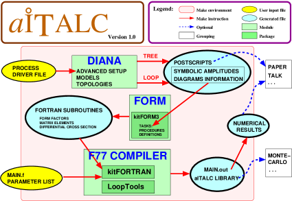
Figure 1: Logical flow chart structure for aITALC.

Despite of the simplicity, the idea of calculating a process by a make instruction has another major advantage: reproducibility, being understood as the ability to recreate once and again similar processes for testing or cross-checking purposes. On the contrary, customizing of an specific process turns out to be a task spread among different parts: driver file, add-on files for neglecting the default ones and specific commands in the main fortran programs.

We will dedicate next parts to a deeper discussion of how each module addresses its tasks and the description of the modus operandi.

5 Feynman diagram generation with Diana

Let us introduce some basic concepts about Diana. If we are thinking of some process, a very intuitive approach is to draw some Feynman diagrams to get a feeling and support the calculation which comes later.

Such a task is very likely to be implemented with the help of computers since it is basically a combinatorial problem. Once we define a model, the external particles, and the level of loops, the problem can be solved. Indeed, Diana will do it for us.

5.1 Basic driver file: Input

The driver file (e.g. process.ini) serves as basic input. It contains primarily:

• physical model,

• incoming and outgoing particles,

• process control flags and options.

These items are used in the Diana “create” file, that will serve as main user input stream for Diana at each level, i.e, tree or loop. Only the number of loops is left to be arranged and written by the Makefile on the “create”. For example, it is compulsory to check and agree with the five lines

SET _processname=muon_production
...
\Begin(model,EWSM.model)
...
ingoing le(;p1),Le(;p4);
outgoing lm(;-p2),Lm(;-p3);
...
options=notadp,onshell;

in process.ini before creating any process. For the case of $\mu$-pair production, as considered in the previous lines, the full driver file is shown in the Fig. 2. Only one remark at this point: special care is needed with the momenta definitions. They all should be assigned to be incoming and clockwise indexed (e.g. p1 addressed to be the first incoming particle, -p2 to be the first outgoing one and so on), so we ensure a matching with the convention used in the predefined topologies.

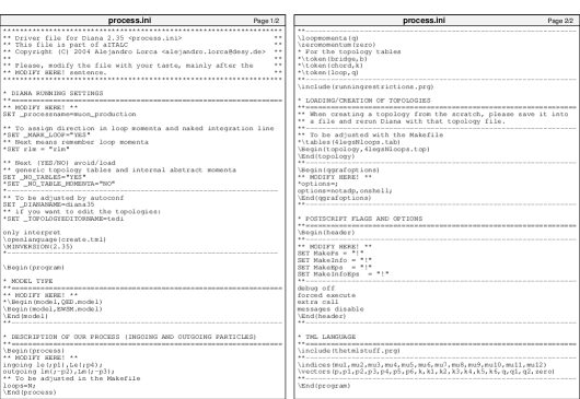
Figure 2: Snapshot for process.ini driver file.

The comment character is * and the ** MODIFY HERE! ** sentences indicate where some modifications are accepted. Regarding the flags for the initial settings, the topology editor (Tedi) can be launched at running time by uncommenting the line:
*SET _TOPOLOGYEDITORNAME ="tedi".

5.2 Implemented models

Once the driver file is fully set up, Diana is able to offer some of the information to Qgraf and, by looking to the allowed couplings given in the model file, create the possible diagrams appearing at each level. The presently available model files are QED.model and EWSM.model. They are summarized in Tab. 5 and Tab. 6.

Both of these models share basic properties according to their phenomenological content. We can distinguish between the following sections:

• Propagator definitions, with general structure
  [ Particle , Antiparticle ; Prototype ; Function ( Prop-label , arguments )* factor ; Mass-sq. ]

  • Boson, e.g. [Wm,Wp ;W; VV(num,ind:1 ,ind:2 ,vec, 2)*i_ ;MMW]

  • Fermion, e.g. [le,Le;l; FF(num,fnum,vec, Mle)*i_; MMle]

  • Ghost, e.g. [ghZ,GhZ; Z ; SS(num,1)*i_; MMZ]

• Vertex definitions, as
  [Interacting particles;;Function(arguments)*factor]

in which the specific Feynman rules will act later. They are, to some extent, part of the model but, from a computational point of view, they belong to the module controlled by Form programs and therefore encoded in a procedure (ctfeynmanrules).

5.3 Topology editor

Tedi is designed to allow the user ultimate flexibility on topology naming, shaping and even defining momenta. It was developed together with Diana as a tool for dealing with topological issues of the Feynman diagrams, and requires the X window server being running in your system. The ‘windows’ and ‘tab’ structure renders an intuitive use, as it is shown in Fig. 3. Furthermore, help and printing facilities are also embedded in the program.

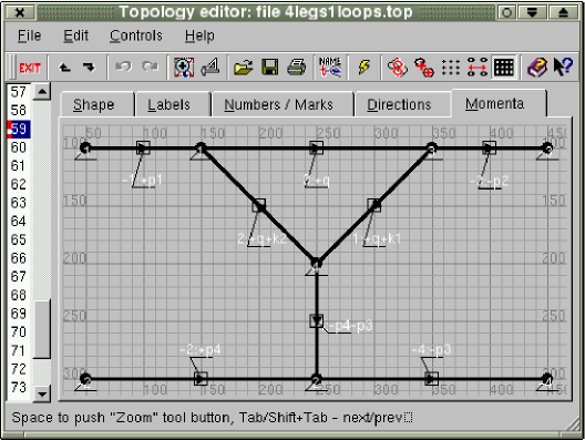
Figure 3: Snapshot for the momenta tab in Tedi.

The content of the five tabs has to do with

• Shape: handles with the aesthetics of the Feynman diagrams. Here the users can reshape the different legs and loops of the topology according to an optimized algorithm or their own taste. Aligning to a grid is also possible by adapting the alignment distance and toggling the key points between nodes for each object.

• Labels: External legs, internal propagators and vertices are given a label in Diana. The location of this label might be varied with respect to the graph to avoid non-legible superpositions.

• Numbers/Marks: Every line has an index that is negative for external legs and positive for internal propagators. Working with this tab one can ensure to give the highest index values to a loop or to fixed-momenta lines.

• Directions: The sign of the momentum flow in each internal line can be flipped by clicking on the arrow with the right-button mouse.

• Momenta: Alternative symbols can be arranged for the momenta attribute.

Apart from this main five features, a bar on the left scrolls between the different topologies that were generated for the specific process.

A deeper discussion of the possibilities of Tedi is out of the focus of a standard aITALC description. Indeed it has been chosen that the default running of any of the examples does not require the topology editor at any moment. We will close this summary with the Fig. 4 in order to give the user an impression of the standard graphical output of Tedi.

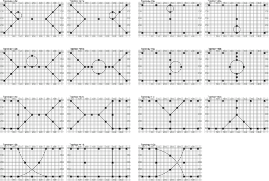
Figure 4: Collection of topologies given by Tedi for the Bhabha scattering at one-loop level. Tadpoles on vertices account for counterterms diagrams.

5.4 Advanced setup

But what if we want to exclude some couplings or modify the aspect of the diagrams?

After the installation of aITALC  it is also possible to use Diana as an independent package. We will show shortly the tested modifications that can be performed at this level.

After running an example (e.g. muon_production), inside the tree directory (also the loop directory in other examples) it is possible to select some files to be considered instead of the default ones coming from the following directory: $AITALCHOME/diana/prg/. This is automatically done by placing those files on the examples/muon_production/ directory and remaking the process. When the process has to be run for the second time, the instructions are: make clean and then make again.

We do not suggest to copy and modify any other file from prg since they are mostly functions using advanced Diana declarations. The following files are welcomed to be modified:

• particleaspect.prg: Defines how every propagator and particle label looks like in the .ps and .eps files. Syntax is not described (just a couple of comments), but intuitive. The field label CT is assigned to counterterms.

• runningrestrictions.prg: Fields or couplings can be excluded here, by uncommenting or replacing them where desired.

5.5 What do we get?

Table 1: Listing for the tree directory inside the muon production example.

alorca@linux:~AITALCHOME/examples/muon_production/tree> ls -XFl total 183 drwxr-xr-x 2 alorca th 2048 Oct 14 15:02 EPS/ drwxr-xr-x 2 alorca th 2048 Oct 14 15:02 FFmuon_production/ drwxr-xr-x 2 alorca th 2048 Oct 14 15:02 InfoEPS/ -rw-r--r-- 1 alorca th 3291 Oct 14 15:02 Makefile -rw-r--r-- 1 alorca th 3710 Oct 14 15:02 muon_production.cnf -rw-r--r-- 1 alorca th 20 Oct 14 15:02 fermioncurrentsnames.in -rw-r--r-- 1 alorca th 3870 Oct 14 15:02 muon_production.in -rw-r--r-- 1 alorca th 4531 Oct 14 15:02 Make_kit.log -rw-r--r-- 1 alorca th 149 Oct 14 15:02 Makefile.log -rw-r--r-- 1 alorca th 1088 Oct 14 15:02 do_amplitude.log -rw-r--r-- 1 alorca th 245 Oct 14 15:02 joinff.1.log -rw-r--r-- 1 alorca th 1059 Oct 14 15:02 joinff.log -rw-r--r-- 1 alorca th 629 Oct 14 15:02 joinkinematics.log -rw-r--r-- 1 alorca th 121102 Oct 14 15:02 joinmm.log -rw-r--r-- 1 alorca th 14779 Oct 14 15:02 muon_production.ps -rw-r--r-- 1 alorca th 18277 Oct 14 15:02 muon_productionInfo.ps

Let’s have a look into the level directory (e.g. tree/ or loop/ as in Tab. 1): the organizer file is called Makefile. It has the instructions to create, organize and fill the different directories by given commands under the Make environment. This means that in order to build the process, only a make instruction is needed. Depending on the process, modifications, hardware and compiler the time for each module varies from seconds till several minutes. At the beginning and end of each module, time stamps are placed in the Makefile.log file at Tab. 1.

The directory also offers Form processed files that we will discuss later. At the moment we can concentrate in just two aspects:

• Graphical representation
  The global files $processname.ps and $processnameInfo.ps summarize all the Feynman graphs appearing at the process. In the EPS/ (and EPSInfo/) directories one may find .eps files with all individual diagrams (and momenta-label definition). Fig. 5 represents the two types of output for a single vertex diagram for the $t$-channel exchange in Bhabha scattering.

• Diagram info
  As it comes out of Diana, the file $processname.in contains the required information about both, global process and individual diagrams. Besides a compulsory expression for the amplitude, specially useful for the Form routines are the preprocessed variables defined for each diagram. Below we show the connection between the Fig. 5 and the corresponding output in $processname.in.

a)	b)

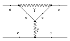
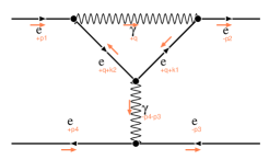
Figure 5: Encapsulated postscripts diagrams for a typical diagram in Bhabha scattering. a) Simple diagram from EPS/ directory, b) also with momenta distribution from InfoEPS/.

*--#[ n11:
****(qgraf number 11)
**** (diagram 11)

#define imm1 "MMle"
#define q1 "-q-k1"
#define loopline1 "1"
#define imm2 "MMle"
#define q2 "-q-k2"
#define loopline2 "1"
#define imm3 "MMA"
#define q3 "+q"
#define loopline3 "1"
#define imm4 "MMA"
#define q4 "+p4+p3"
#define loopline4 "0"

#define k1 "(+p2)"
#define k2 "(-p1)"
...
#define DIAGRAM "11"
#define COUNTER "11"
#define LINE "4"
#define FERMIONLOOP "0"
#define TOPOLOGY "4t1c"
#define CHANNEL "t"
#define SKELETON "1"
#define LOOPTYPE "c"
#define LOOPTYPENUMBER "3"
#define PROTOTYPE "llaa"
#define FERMIONCHANNEL "T"
#define l1 "1"
#define l2 "2"
#define l3 "1"
#define l4 "2"
*-----------------------------------------
g [Amplitude,11] =
       (-1)*F(3,1,mu2,1,0,1)*(-i_)*e*Qle*FF(1,1,-q-k1,Mle)*i_*
       F(4,1,mu4,1,0,1)*(-i_)*e*Qle*FF(2,1,-q-k2,Mle)*i_*
       F(1,1,mu1,1,0,1)*(-i_)*e*Qle*F(2,2,mu3,1,0,1)*(-i_)*e*Qle*
       VV(3,mu1,mu2,+q,0)*i_*VV(4,mu3,mu4,+p4+p3,0)*i_;

*--#] n11:

6 Algebra manipulation: Library in Form

The form module acts as a bridge connecting the world of the purely symbolic representation of the Feynman diagrams, directly read off the lagrangian, and the numerical description of a scattering problem of real particles.

When Diana has finished one of the levels, a complete description of the process is obtained, but still in an encoded language. Different Form programs will prepare the amplitudes in order to render numerically evaluable expressions. Tracing, commuting $\gamma$ matrices, applying the Dirac equation to external fermions or introducing the Mandelstam variables is part of this module.

There are basically two kind of programs: The main routines and the procedures. We describe the four routines:

• do_amplitude.frm: Attempts to simplify the individual amplitude for each diagram, extracting out the form factors in a given basis of matrix elements.

• joinkinematics.frm: Defines how the differential cross section should be composed in terms of fermion currents (S, T or U), the normalization of the incoming flux in the cross section formula, soft photon emission and the definition of the Mandelstam variables.

• joinmm.frm: The standard set of matrix elements is considered by this program, giving, as output, the multiplication of any two elements appearing in the amplitude decomposition.

• joinff.frm: Once all the diagrams were considered, this part pastes together the form factor contributions sorted by topologies. The final translation into Fortran code is also done at this step.

6.1 Procedures in kitFORM3/

The listing of the procedures is long, and the description of each of them is shortly presented in Tab. B.

At least we would like to draw the attention to one option regarding the neglect of the external masses of particles (e.g. light fermion masses). This can be achieved including the adapted Neglectedmasses.inc file into the main directory, together with the driver file process.ini.

Coming back to our previous listing of the directory at Fig. 1, in the files do_amplitude.log and joinmm.log we find information about the individual evaluation of each diagram and the kinematical factor corresponding to the cross product of matrix elements, respectively. Also, extra functions related to soft photon emission, flux factors and Mandelstam variables can be found in joinkinematics.log. As an intermediate step, individual amplitudes are stored in the FF$processaname/ directory.

7 Getting numbers: the Fortran code

So far the expressions that were generated contain large amount of analytical work on them. Now one has to execute them and evaluate the parameters, loop integrals and finally retrieve finite formfactors that, clustered by topologies, will allow together with the matrix elements to calculate the cross section for a given process.

The structure of the fortran module can be outlined as follows:

• main.f, parameterlist.hf: they both give the user access to modify the output structure of the program and the explicit values of the model respectively. In the main.f file we find many settings as logical flags, input of kinematics and output control.

• kitFORTRAN: consists of the full set of Fortran subroutines and functions needed to compile the main.f program. We can divide them into two categories, according to the role they play during running time.

  • Global are those that were fixed at installation time and considered to be process independent. They are stored at $AITALCHOME/fortran/src

  • Local are written at running time by the tree and loop modules and depend explicitely on the application. They get placed at $processname/fortran/src.

• LoopTools: this library is called with the purpose of numerically calculating the most of the loop integrals.

7.1 Understanding and controlling the output

A sample output are the Tabs. 2 and 3 with differential cross sections (given always in pb). The first column corresponds to the beam energy ($\sqrt{s}=\mathtt{setsqrtsman}$) given in GeV, the second one to the $\cos\theta$ (setcost), $\theta$ being the angle between the three-momenta $\mathbf{p_{1}}$ and $-\mathbf{p_{2}}$. Later on we have successively the columns of the Born approximation (Born), the interference terms of the tree and loop levels (loop) and the soft photonic corrections (soft). These three columns (third, fourth and fifth) are summed into the sixth column (B+corr) with the finally corrected cross section. The last column loop^2 contains the one-loop squared terms in the perturbative approach. The maximum energy fraction that the soft photon may gain out of $\sqrt{s}$ is limited by the variable setfracomega.

Table 2: File main.log, for the bhabha_QED example.

#=============================================================================================
# aITALC Version 1.0 (29.10.2004) by A.Lorca -- T.Riemann
#---------------------------------------------------------------------------------------------
#sqrtsman      cost      dcs(Born)     dcs(loop)     dcs(soft)     dcs(B+l+s)    dcs(loop^2)
 0.5000000E+03 -.9000000 0.5238736E+00 0.1045142E+00 -.2193133E+00 0.4090746E+00 0.9235446E-02
 0.5000000E+03 -.5000000 0.6116007E+00 0.1767866E+00 -.2922801E+00 0.4961073E+00 0.1727483E-01
 0.5000000E+03 0.0000000 0.1172536E+01 0.3974063E+00 -.6065847E+00 0.9633579E+00 0.4206711E-01
 0.5000000E+03 0.5000000 0.5504406E+01 0.2126643E+01 -.3064635E+01 0.4566414E+01 0.2405476E+00
 0.5000000E+03 0.9000000 0.1891184E+03 0.8703341E+02 -.1165000E+03 0.1596518E+03 0.1089656E+02
#=============================================================================================
#Energy given in GeV, Cross sections in pb, setfracomega= 0.1000000

Table 3: File main.log, for the leLe.bS example.

#=============================================================================================
# aITALC Version 1.0 (29.10.2004) by A.Lorca -- T.Riemann
#---------------------------------------------------------------------------------------------
#sqrtsman      cost      dcs(Born)     dcs(loop)     dcs(soft)     dcs(B+l+s)    dcs(loop^2)
 0.5000000E+03 -.9000000 0.0000000E+00 0.0000000E+00 0.0000000E+00 0.0000000E+00 0.6534118E-08
 0.5000000E+03 -.5000000 0.0000000E+00 0.0000000E+00 0.0000000E+00 0.0000000E+00 0.7095421E-08
 0.5000000E+03 0.0000000 0.0000000E+00 0.0000000E+00 0.0000000E+00 0.0000000E+00 0.1048690E-07
 0.5000000E+03 0.5000000 0.0000000E+00 0.0000000E+00 0.0000000E+00 0.0000000E+00 0.2084942E-07
 0.5000000E+03 0.9000000 0.0000000E+00 0.0000000E+00 0.0000000E+00 0.0000000E+00 0.4643956E-06
#=============================================================================================
#Energy given in GeV, Cross sections in pb, setfracomega= 0.1000000

If the calculation is correct, all the columns should be constant under variation of the ultraviolet (UV) parameter (you can check this by turning on the flag luvcheck). The same check for the infrared (IR) behaviour (lricheck) will change the explicit values in columns loop and soft, but the sum should still be invariant. The last column may also suffer against IR variation since it is neither compensated by double soft photon emission nor two-loop divergencies. Those loop^2 numbers are crucial when they become the leading order in e.g. flavour changing neutral current processes (FCNC) as discussed in [8], or just as an estimator of the order of magnitude for the error in the next level of perturbation theory. When integrated cross sections are under study, the integration region is limited by the setlimcost variable, the ics and fba being defined in terms of dcs as

$$\mathtt{dcs} = \frac{\d{\sigma}}{\d\cos{\theta}}$$ (1)

$$\mathtt{ics} = \sigma_{\mathrm{tot}}=\int_{-\mathtt{setlimcost}}^{\mathtt{setlimcost}}\!\!\!\!\d\cos{\theta}~{}\mathtt{dcs}$$ (2)

$$\mathtt{fba} = \frac{\sigma_{\mathrm{fw}}-\sigma_{\mathrm{bw}}}{\sigma_{\mathrm{tot}}}=\int_{0}^{\mathtt{setlimcost}}\!\!\!\!\d\cos{\theta}~{}\frac{\mathtt{dcs}}{\mathtt{ics}}-\int_{-\mathtt{setlimcost}}^{0}\!\!\!\!\d\cos{\theta}~{}\frac{\mathtt{dcs}}{\mathtt{ics}}.$$ (3)

The integration algorithm is based on a Richardson extrapolation to the Romberg integration [9] with four steps. The estimated error is supplied in short forms in extra columns. If it does not suffice or for cross checking, the same subroutine with eight steps (ICS8) can be called instead of the faster ICS. A complete survey of variables is presented in Tab. C.

7.2 A greedy possibility: quadruple precision

Not every compiler allows for extended or quadruple precision. This is a feature outside of the ANSI Fortran77. Even if aITALC contains some code’s implementations outside the ANSI syntax, they are quite common (e.g. using underscore, or double complex), so decent compilers won’t complain.

But on high level computation, or simply as comparison, switching on the quadruple precision could stabilize numerical results or render amazing agreement with other calculations.

8 Examples including loop level

To finish this descriptive chapter, we would like to present the examples available with the distribution.

The package is delivered with three examples that the user may run without further considerations. In the directory examples/ we have the following processes:

• $\mu$-pair production at tree level: $e^{-}e^{+}\rightarrow\mu^{-}\mu^{+}$

• Bhabha scattering in QED (see [10]): $e^{-}e^{+}\rightarrow e^{-}e^{+}$

• Fermion Flavour Violation example: $e^{-}e^{+}\rightarrow b\bar{s}$

under the directory names of muon_production, Bhabha_QED and leLe.bS.

Table 4: Typical timings for the different modules. The technical specifications for system Laptop are: Intel Centrino 1.5GHz cpu, 512MB RAM, Intel icc and ifort version 8.1 compilers. For Desktop: Intel Pentium III 853MHz cpu, 256MB RAM, GNU gcc and g77 version 3.3.3 compilers.

	muon_production		leLe.bS		bhabha_QED
Module	Desktop	Laptop	Desktop	Laptop	Desktop	Laptop
tree	9”	3”	4”	1”	30”	9”
loop	–	–	2’20”	52”	37”	12”
fortran	15”	4”	4:35’56”	33”	26”	8”
Total	24”	7”	4:38’20”	1’26”	1’33”	29”

Running time expected for the execution of all the examples were studied on two different computers. The results are shown in Tab. 4. One can see that when the size of the Fortran code begins to be large (i.e. more than $\sim$200kB for a single subroutine to be compiled), then the required time for the GNU compiler gets too long, compared to the other processes or compiler.

Appendix A Implemented models

Table 5: Particle content of the QED model (QED.model)

Code		Arguments	Particle	Name	Lorentz type
Lepton
le ,	Le	(;$p_{i}$)	$e^{-}$, $e^{+}$	electron, positron	fermion
Gauge boson
A		($\mu_{i}$;$p_{i}$)	$\gamma$	photon	boson

Table 6: Particle content of the electro-weak sector in the standard model (EWSM.model)

Code		Arguments	Particle	Name	Lorentz type
Leptons
ne ,	Ne		$\nu_{e}$, $\bar{\nu}_{e}$	neutrino-$e$, antineut-$e$
nm ,	Nm	(;$p_{i}$)	$\nu_{\mu}$, $\bar{\nu}_{\mu}$	neutrino-$\mu$, antineut-$\mu$	fermion
nt ,	Nt		$\nu_{\tau}$, $\bar{\nu}_{\tau}$	neutrino-$\tau$, antineut-$\tau$
le ,	Le		$e^{-}$, $e^{+}$	electron, positron
lm ,	Lt	(;$p_{i}$)	$\mu^{-}$, $\mu^{+}$	muon, antimuon	fermion
lt ,	Lt		$\tau^{-}$, $\tau^{+}$	tau, antitau
Quarks
u ,	U		$u$, $\bar{u}$	up, antiup
c ,	C	(;$p_{i}$)	$c$, $\bar{c}$	charm, anticharm	fermion
t ,	T		$t$, $\bar{t}$	top, antitop
d ,	D		$d$, $\bar{d}$	down, antidown
s ,	S	(;$p_{i}$)	$s$, $\bar{s}$	strange, antistrange	fermion
b ,	B		$b$, $\bar{b}$	bottom, antibottom
Gauge bosons
A			$\gamma$	photon
Z		($\mu_{i}$;$p_{i}$)	$Z$	Z-boson	vector
Wm ,	Wp		$W^{-}$, $W^{+}$	W-boson
Higgs sector
H			$H$	Higgs
G0		(;$p_{i}$)	$\chi$	would-be	scalar
Gm ,	Gp		$\phi^{-}$, $\phi^{+}$	Goldstone bosons
Faddeev-Popov ghosts
ghA ,	GhA		$\eta_{\gamma}$, $\bar{\eta}_{\gamma}$	photon ghosts	scalar
ghZ ,	GhZ	(;$p_{i}$)	$\eta_{Z}$, $\bar{\eta}_{Z}$	Z-ghosts	with
ghm ,	Ghm		$\eta_{W^{-}}$,$\bar{\eta}_{W^{-}}$	W--ghosts	fermion
ghp ,	Ghp		$\eta_{W^{+}}$, $\bar{\eta}_{W^{+}}$	W+-ghosts	statistics

Appendix B List of Form procedures

Table 7: Different procedures used.

Name	Args.	Description
LTtoPV		Translates the indexing of loop integrals from [11] into [12] convention.
aitalcnotation	$N$	Translates the Form code into Fortran readable. The argument $N=1$ allows for complex masses while $N=0$ does not
analyzeterms		Part of simplifygrams
argsymmetries		Applies symmetry properties on arguments for loop functions and Gram determinants
canceldens		To cancel composition of den(a,b)*(a-b)=1
chisholm		Applies Chisholm identities by converting all chains of $\gamma$ matrices that are contracted by their dimensional value
contgammas		Simplifies contractions in products of gamma matrices
contractepsilon		It contracts the product of two $\epsilon$ tensors
ctfeynmanrules		Insertion of Feynman rules with counterterms
definegrams		Defines a Form global variable with the explicit expression of a Gram determinant
derivateself		Derivates self-energy functions
dimensionfour		To reach the limit $D\to 4$ taking care of the UV-behaviour of scalar integrals
diracequation		Applies Dirac equation to available spinors
dummytovar	$N$	Part of simplifygrams. $N$ stands for the amount of arguments in dummyN function
equalindex		Gives the same index to potentially different contractions keeping them ordered by number
externalmomenta		To substitute the internal momenta in loops with external ones
gamma3to1		Introduces an $\epsilon$ tensor and $\gamma_{5}$ to remove the product of three $\gamma$’s
gammaalgebra		Prepares $\gamma$ chain structures for diracequation
gammamunu		Introduces indices in the vector structures
gramback	$N$	Part of simplifygrams. Returns the Gram determinant of order $N$ if no simplification was found
gramsubstitution	$N,w$	It substitutes the $w$-element to match posssible order $N$ Gram determinants
identifyintegrals		Picks up the different loop integrals and provides a set of Form $-variables with the right substitutions, inserting the function LoopIntegral=LI(n)
integrationde93		Procedure to integrate 4,3,2,1-point functions with internal momenta decomposition like in [11]
invgammamunu		Undoes the gammamunu effects
keepUVloops		Keeps only integrals actually UV divergent
loopsymmetries		Minimize loop integrals in boxes by symmetrizing arguments
lorentzinvariants		Adapts scalar product of vectors to Lorentz invariant squared masses
massconvention		To use single variables for the masses with M instead of MM outside arguments
massivefofa	$j,c,N$	Calculates and saves the formfactors as [13]. j stands for topology, c for left-right or $\mathbf{1}$-$\gamma_{5}$ and N=1(0) do (not) print the formfactors
movepslash		Places the desired $\not{p}_{i}$ to the side of fermion chain to apply diracequation
neglectmass	zero	Neglects positive powers of terms as indicated in the file Neglectedmasses.inc. zero is the substituted value
nosymboliccouplings		To put explicit values of charges and weak couplings
onshell		Substitutes external momenta for external particle masses and Mandelstam variables
pslashaway		Reorder away the non desired position of $\not{p}_{i}$
pushgamma5		Pushes $\gamma_{5}$ to the right in fermion chains
pushomegas		Orders and pushes Left or Right projectors ($\omega_{L,R}$) to the right in fermion chains
recoverargumentsde93		Catchs back the arguments of loop integrals in combination with integrationde93
reductionDD02	$N$	Reduction algorithm from scalar tensor integrals to master integrals given in [14]. $N=1$ sorts after each integral type, $N=0$ does not sort at all
reductionLT		reductionDD02(1) with LoopTools notation
simplifygrams		Tries to remove inverse Gram determinants by looking to the numerator (time and memory consuming!)
simplihelp	$N,r$	It helps simplifygrams to run sequentially $r$ times from the highest power of one variable for $N$ order Gram determinants
storeself	$j,c,N$	Stores self energies, j stands for topology, c for ($\omega_{L}$,$\omega_{R}$) or ($\mathbf{1}$,$\gamma_{5}$) and N=1(0) do (not) print the form factors
threegammastoepsilon		Introduces and removes the $\epsilon$ tensor simplifying chains of 3 $\gamma$ matrices that naturally don’t dissappear after diracequation
tracefermiloops		Traces possible fermion loops in self-energies
transvorlongit	$x$	Sets the longitudinal and transverse part of self energies, keeping off-shell but with mass2 argument $x$
unityCKM		Makes $\mathrm{CKM}_{ij}=\delta_{ij}$
usegamma5		Uses $\gamma_{5}$, instead of $\omega_{L,R}$ projectors
useomegas		The opposite to usegamma5
vartodummy		Part of gramback, opposite as dummytovar

Appendix C Settings for main.f

Table 8: Kinematical and variables and logical flags for different settings in main.f.

Variable	Type	Def. value	Meaning
Kinematical
icostloop	integer	5	Dimension of setcostarray
isqrtsloop	integer	5	Dimension of setsqrtsmanarray
setcostarray	double	data //	Set of default values for the setcost ($\cos{\theta}$) do loop in the dcs evaluation
setsqrtsmanarray	double	data //	Set of default values for the setsqrtsman ($\sqrt{s}$) do loop in the ICS evaluation
setfracomega	double	0.1d0	Limit for the maximum soft photon energy
setlimcost	double	.9999d0	Limit of integration for ics and fba
Process flags
lrenorm	logical	.true.	Call the renormalization subroutine to calculate the counterterms parameters
lwidth	logical	.false.	Call the loop integrals with complex values for boson masses. For the four-point integral, only the case with one massless boson (photon) is considered.
lidentCKM	logical	.false.	Brings the CKM mixing matrix in a diagonal form, so no mixing occurs
Checking flags
luvcheck	logical	.false.	Perform a shift in the mudim and delta parameters in LoopTools
lircheck	logical	.false.	Perform a shift in the lambda parameter in LoopTools
Output flags
lcostloop	logical	.true.	Performs a do-loop over setcost
lprintics	logical	.false.	Performs a do-loop over setsqrtsman and prints the results of ics
lprintfba	logical	.false.	Performs a do-loop over setsqrtsman and prints the results of fba
llongoutput	logical	.false.	Prints the cross sections in double precision format

References

-
[1]
M. Tentyukov and J. Fleischer,
Comput. Phys. Commun. 132 (2000) 124,
hep-ph/9904258,
Available at
http://www.physik.uni-bielefeld.de/~tentukov/diana.html. -
[2]
P. Nogueira,
An introduction to Qgraf 2.0,
Available at
ftp://gtae2.ist.utl.pt/pub/qgraf. -
[3]
J.A.M. Vermaseren,
math-ph/0010025,
Available at
http://www.nikhef.nl/~form. -
[4]
T. Hahn and M. Perez-Victoria,
Comput. Phys. Commun. 118 (1999) 153,
hep-ph/9807565,
LoopTools available at
http://www.feynarts.de/looptools. -
[5]
G.J. van Oldenborgh,
Comput. Phys. Commun. 66 (1991) 1,
Available at
http://www.xs4all.nl/~gjvo/FF.html. - [6] J. Fleischer et al., Eur. Phys. J. C31 (2003) 37, hep-ph/0302259, Code reachable via http://www.ifh.de/~riemann/doc/topfit/topfit.html.
-
[7]
A. Lorca and T. Riemann,
aITALC an Integrated Tool for Automated Loop Calculations, version
1.0 (29 October 2004),
Available at
http://www.ifh.de/theory/aitalc/downloads/doc/aitalc-1.0.pdf. - [8] A. Lorca and T. Riemann, Nucl. Phys. B (Proc. Suppl.) 135 (2004) 328, hep-ph/0407149.
- [9] W.H. Press et al., Numerical Recipes in FORTRAN: The Art of Scientific Computing, 2nd ed. (Cambridge University Press, Cambridge, U.K., 1992) chap. 4.3 Romberg integration, and 16.4 Richardson Extrapolation and the Bulirsch-Stoer Method, pp. 134–135 and 718–725.
- [10] J. Gluza, A. Lorca and T. Riemann, Nucl. Instrum. Meth. A534 (2004) 289, hep-ph/0409011.
- [11] A. Denner, Fortschr. Phys. 41 (1993) 307.
- [12] G. ’t Hooft and M.J.G. Veltman, Nucl. Phys. B153 (1979) 365.
- [13] A. Lorca, Ph.D. thesis, Universität Bielefeld, Bielefeld, Germany, 2005, In preparation.
- [14] A. Denner and S. Dittmaier, Nucl. Phys. B658 (2003) 175, hep-ph/0212259.