Introduction

The investigation of the quark-gluon dynamics through perturbative calculations is most useful to extract from experimentally measurable observables quantities such as parton distributions, generalized parton distributions (GPDs) and (generalized) distribution amplitudes (GDAs, DAs). Factorization theorems allow to calculate scattering amplitudes in a perturbative way, provided a renormalization scale and a factorization scale are choosen. Whereas the observables in the extensively studied inclusive reactions are in general related to an amplitude (as the case of inclusive DIS expressed as the imaginary part of the forward virtual Compton scattering reaction), exclusive cross sections which have been much studied recently are based on a factorization theorem at the amplitude level, and thus require to square the amplitude given by its perturbative expansion. Renormalization scale fixing has been the subject of intense studies and different strategies [1, 2] have been put forward to maximize the predictivity of theoretical studies through ensuring the smallness of corrections related to higher orders terms in the perturbative series. The phenomenological success of these proposals is quite impressive in a number of cases, mostly related to inclusive cross sections or jet physics. With the advent of next to leading order results, it has been advocated to use these procedures also in hard exclusive processes [3, 4]. Even at the Born level, the hard meson electroproduction amplitude contains $\alpha_{S}$. Therefore the choice of the renormalization scale $\mu_{R}$ is very crucial for the practical estimations of the observables related to meson electroproduction. The first study of a hard electroproduction amplitude including the analysis of the next-to-leading orders (NLO) has been implemented by Belitsky and Muller [3] for $\pi^{+}$ production, i.e. for $\gamma^{*}p\to\pi^{+}n$ process. This study used an appropriate continuation of the NLO calculations known for the electromagnetic pion form factor [5] onto the case of the meson electroproduction process.

In this work, focusing on the Brodsky-Lepage-Mackenzie (BLM) procedure [2] , we examine in detail the consequences of the fact that exclusive processes considered in the regime where the quark GPDs are dominant are factorized at the amplitude level and that the meson electroproduction amplitude is a complex function. Consequently, we are forced to apply the BLM procedure to the real and to the imaginary part of the scattering amplitude separately, which in general leads to two different scales. Moreover, we show that such a way of scale fixing, as has been done in [3] for the $\pi-$meson production, leads to unphysical results in case of vector meson production. We propose a way to modify the BLM procedure in order to avoid such difficulties.

Basics of the BLM procedure

The QCD factorization theorem [6] states that the amplitude of hard meson electroproductions can be written as

$${\cal A}=\int\limits_{0}^{1}dz\int\limits_{-1}^{1}dx\,\Phi_{M}(z,\mu^{2}_{F})\,H(x,z,Q^{2},\mu^{2}_{F},\mu^{2}_{R})\,F(x,\mu^{2}_{F})\equiv\Phi_{M}\,\otimes\,H\,\otimes\,F,$$ (1)

where the parameters $\mu_{F}^{2}$ and $\mu^{2}_{R}$ are the factorization and renormalization scales, respectively. The scales $\mu_{R}^{2}$ and $\mu_{F}^{2}$ are in principle independent but often it is argued that they can coincide, $\mu_{R}^{2}=\mu_{F}^{2}$. The arguments in favour of such assumption are discussed in, e.g. [7], and we adopt this also in the present paper (to simplify notation we omit below subscripts $R$ and $F$). In Eq.(1), $H$ is the hard part of amplitude which is controlled by perturbative QCD. The meson distribution amplitude $\Phi_{M}$ describes the transition from the partons to the meson, and $F$ denotes the GPDs which are related to nonperturbative matrix elements of bilocal operators between different hadronic states.

The product $\Phi_{H}\,\otimes\,H\,\otimes\,F$ in (1) is, generally speaking, independent of the particular choice of the parameter $\mu^{2}$. However, this independence is broken once we limit ourselves to the first few terms in an expansion over the coupling constant $\alpha_{S}$. In this case, the theoretical ambiguity of the choice of the parameter $\mu^{2}$ emerges. The goal is to choose the parameter $\mu^{2}$ such as to ensure that pretty small contributions will arise from the next order corrections. Out of the several possible ways to hope to reach that goal, the BLM procedure [2] begins with separating out the terms which are proportional to the one-loop $\beta-$function, $\beta_{0}=11-2/3N_{F}$, appearing in the NLO terms. The amplitude (1) including the NLO corrections with separated terms proportional to $\beta_{0}$ reads

$${\cal A}=\alpha_{S}(\mu^{2})\,{\cal A}^{{\rm LO}}(Q^{2})+\alpha_{S}^{2}(\mu^{2})\,\frac{\beta_{0}}{4\pi}\Biggl{\{}\biggl{[}C-{\rm ln}\frac{Q^{2}}{\mu^{2}}\biggr{]}\,{\cal A}^{{\rm LO}}(Q^{2})+\tilde{\cal A}^{{\rm NLO},(\beta)}(Q^{2})\Biggr{\}}+...,$$ (2)

where the ellipsis stand for the terms of the NLO corrections which do not explicitly contain $\beta_{0}$. In (2), the value of the constant $C$ depends on the kind of produced mesons. As pointed out in [3], [5] the exact expressions, in the quark sector, with the NLO corrections may be obtained by a suitable substitution from the well-known results for the pion electromagnetic form factor.

Due to the renormalization group equations the coupling constant takes the form

$$\alpha_{S}(\mu^{2})=\frac{1}{(\beta_{0}/4\pi)\,{\rm ln}(\mu^{2}/\Lambda^{2}_{QCD})}=\frac{\alpha_{S}(\mu^{2}_{0})}{1+(\beta_{0}/4\pi)\,\alpha_{S}(\mu^{2}_{0})\,{\rm ln}(\mu^{2}/\mu^{2}_{0})}.$$ (3)

We insert this expression into the amplitude (2) and then expand it in powers of $\alpha_{S}(\mu^{2}_{0})$. Retaining the terms which are proportional to $\beta_{0}$, we get

$${\cal A}=\alpha_{S}(\mu^{2}_{0})\,{\cal A}^{{\rm LO}}(Q^{2})-\alpha_{S}^{2}(\mu^{2}_{0})\,\frac{\beta_{0}}{4\pi}\,{\rm ln}\frac{\mu^{2}}{\mu^{2}_{0}}\,{\cal A}^{{\rm LO}}(Q^{2})+$$

$$\alpha_{S}^{2}(\mu^{2}_{0})\,\frac{\beta_{0}}{4\pi}\Biggl{\{}\biggl{[}C-{\rm ln}\frac{Q^{2}}{\mu^{2}}\biggr{]}\,{\cal A}^{{\rm LO}}(Q^{2})+\tilde{\cal A}^{{\rm NLO},(\beta)}(Q^{2})\Biggr{\}}+...$$ (4)

The BLM procedure consists in the choice of such $\mu_{0}^{2}$ for which the whole term proportional to $\beta_{0}$ in Eq. (Basics of the BLM procedure) vanishes, i.e.

$$\alpha_{S}^{2}(\mu^{2}_{0})\,\frac{\beta_{0}}{4\pi}\,{\rm ln}\frac{\mu^{2}}{\mu^{2}_{0}}\,{\cal A}^{{\rm LO}}-\alpha_{S}^{2}(\mu^{2}_{0})\,\frac{\beta_{0}}{4\pi}\Biggl{\{}\biggl{[}C-{\rm ln}\frac{Q^{2}}{\mu^{2}}\biggr{]}\,{\cal A}^{{\rm LO}}+\tilde{\cal A}^{{\rm NLO},(\beta)}\Biggr{\}}=0,$$ (5)

from which it follows that the BLM scale $\mu^{2}_{BLM}$ is equal to

$$\mu^{2}_{0}=\mu^{2}_{BLM}=Q^{2}\,e^{-f},\quad f=C+\frac{\tilde{\cal A}^{{\rm NLO},(\beta)}}{{\cal A}^{{\rm LO}}}.$$ (6)

If the scattering amplitude is real, as in the case of the spacelike pion form factor, the above procedure leads just to the one $\mu^{2}_{BLM}$ scale. But already in the $\pi^{+}-$meson electroproduction the scattering amplitude is a complex function and if one applies the BLM procedure separately both for real and imaginary parts , this results in two different scales. The situation starts to be even worse in the case of the vector meson electroproduction which we discuss in the next section.

Extraction of the BLM scale from the amplitudes

We now focus on the numerical estimation of the renormalization scales extracted them from the amplitudes of the vector mesons electroproduction. We consider only spin non-flip quark GPD $H$ of the nucleon target and neglect spin-flip GPD $E$. The reason is that: a) $E$ function gives very small contribution to the scattering amplitude, b) its form is very model dependent.

Consider the NLO terms of amplitude (2) containing the $\beta_{0}$ coefficient

$$\biggl{[}C-{\rm ln}\frac{Q^{2}}{\mu^{2}}\biggr{]}\,{\cal A}^{{\rm LO}}(Q^{2})+\tilde{\cal A}^{{\rm NLO},(\beta)}(Q^{2})\sim\int\limits_{0}^{1}dz\,\int\limits_{-1}^{1}dx\,\left\{\Phi_{\rho}(z)\atop\Phi_{H}(z)\right\}H^{p}(x,\xi,t_{min})$$ (7)

$$\,\biggl{\{}\,\frac{2\xi}{z(\xi+x)}\biggl{[}\frac{5}{3}-{\rm ln}(\frac{z(\xi+x)}{2\xi})-{\rm ln}(\frac{Q^{2}}{\mu^{2}})\biggr{]}\mp(z\to\bar{z};\,x\to-x)\,\biggr{\}}=0.$$

In Eqn. (7), the distribution amplitudes $\Phi_{\rho}(z)$ and $\Phi_{H}(z)$ correspond to the $\rho$ and hybrid mesons, respectively. The hybrid meson is a charge conjugation even state ($J^{PC}=1^{-+}$), as studied in [8]. The function $H^{p}(x,\xi,t_{min})$ stand for the corresponding GPD’s and is defined as

$$H^{p}(x,\xi,t)=\frac{1}{\sqrt{2}}\biggl{(}e_{u}H^{u}(x,\xi,t)-e_{d}H^{d}(x,\xi,t)\biggr{)}.$$ (8)

The meson distribution amplitudes $\Phi_{\rho}$ and $\Phi_{H}$ may be understood as the asymptotic functions which are (see, for instance [8]):

$$\Phi_{\rho}(z)=6z\bar{z},\quad\Phi_{H}(z)=30z\bar{z}(1-2z).$$ (9)

Note that the NLO evolution effects for the meson distribution amplitudes seem to be small and we omit the consideration of such effects.

The GPD’s, in (7), can be modelled using the Radyushkin model [9] which ensures the agreement with the forward limit and the corresponding sum rules for the moments. According to this ansatz, the GPD’s are expressed with the help of double distributions $F^{q}(x,y;t)$:

$$H^{q}(x,\xi,t)=\frac{\theta(\xi+x)}{1+\xi}\int\limits_{0}^{{\rm min}\{\frac{x+\xi}{2\xi},\frac{1-x}{1-\xi}\}}dy\,F^{q}(x_{+},y,t)-\frac{\theta(\xi-x)}{1+\xi}\int\limits_{0}^{{\rm min}\{\frac{\xi-x}{2\xi},\frac{1+x}{1-\xi}\}}dy\,F^{\bar{q}}(x_{-},y,t),$$ (10)

where

$$x_{+}=\frac{x+\xi-2\xi y}{1+\xi},\quad x_{-}=\frac{\xi-x-2\xi y}{1+\xi}.$$ (11)

For the double distribution $F^{q}(X,Y;t)$, we assume the ansatz suggested by Radyushkin [9]:

$$F^{q}(X,Y;t)=\frac{F_{1}^{q}(t)}{F_{1}^{q}(0)}\,q(X)\,6\frac{Y(1-X-Y)}{(1-X)^{3}},$$ (12)

where the forward (anti)quark distribution is taken from the parameretization of [10]. Note that, in (12), $t_{min}$ is different from zero and is equal to $-4m^{2}_{N}\xi^{2}/(1-\xi^{2})$ (see, for instance, [11]). A similar expression gives the anti-quark contribution.

As shown in [12], the definition of the double distribution is not completely compatible with the structure of the corresponding matrix elements; introducing D-terms restores the self-consistency of this representation. Taking into account these D-terms with a factorized $t$-dependence as in Eq. (12), the GPD’s (10) are modified into :

$$H^{q}_{D}(x,\xi,t)=H^{q}(x,\xi,t)+\theta(\xi-|x|)\frac{D(x/\xi,t)}{N_{f}},$$ (13)

where $D(x/\xi,0)$ is given by ($C_{n}^{3/2}$ are Gegenbauer polynomials)

$$D(\alpha)=-4(1-\alpha^{2})\biggl{\{}C_{1}^{3/2}(\alpha)+0.3C_{3}^{3/2}(\alpha)+0.1C_{5}^{3/2}(\alpha)\biggr{\}}$$ (14)

with

$$\alpha=\frac{x}{\xi},\quad D(\alpha)=-D(-\alpha).$$ (15)

These D-terms do contribute to the interval $-\xi<x<\xi$ of the GPD’s. Besides, due to the anti-symmetric properties of (14), the D-terms are important only for the charge conjugation odd vector meson (e.g. $\rho$) production amplitude rather than for exotic hybrid meson ($J^{PC}=1^{-+}$) production amplitude [8].

As aforementioned, the amplitudes of the mesons electroproductions contain real and imaginary parts. So, we now come to the estimation of BLM scales for the real and imaginary parts of amplitudes, separately. Repeating the procedure pointed out in the preceding section, we derive that the BLM scales read

$$\mu^{2}_{(Re)}=\,e^{-f_{Re}(\xi)}\,Q^{2},$$ (16)

$$\mu^{2}_{(Im)}=\,e^{-f_{Im}(\xi)}\,Q^{2},$$ (17)

where

$$f_{Re}^{\rho}(\xi)=\frac{19}{6}-\frac{H^{Re}_{2}(\xi)}{H^{Re}_{1}(\xi)},$$ (18)

$$f_{Im}^{\rho}(\xi)=\frac{19}{6}-\frac{H^{Im}_{2}(\xi)}{H^{Im}_{1}(\xi)}.$$ (19)

for the $\rho$ meson production, and

$$f_{Re}^{H}(\xi)=\frac{9}{2}-\frac{G^{Re}_{2}(\xi)}{G^{Re}_{1}(\xi)},$$ (20)

$$f_{Im}^{H}(\xi)=\frac{9}{2}-\frac{G^{Im}_{2}(\xi)}{G^{Im}_{1}(\xi)}.$$ (21)

for the hybrid meson production. The explicit expressions for functions $H^{Re}_{i}(\xi)$, $H^{Im}_{i}(\xi)$, $G^{Re}_{i}(\xi)$ and $G^{Im}_{i}(\xi)$ in (18)–(21) can be found in the Appendix.

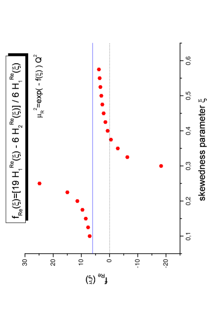
Figure 1: The $\rho$ meson production: the BLM scale for the real part of the amplitude.

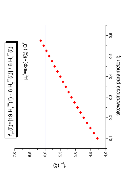
Figure 2: The $\rho$ meson production: the BLM scale for the imaginary part of the amplitude.

The investigation of the $\rho$ meson scale with (18) shows that the extraction of the BLM scale from the expression for the amplitude meet difficulties. Indeed, as one can see on Fig. 1, the $\rho$ meson function $f_{Re}^{\rho}(\xi)$ has an unphysical singularity owing to the fact that the denominator in (18) may vanish (see the exact expression for $H^{Re}_{i}(\xi)$ in Appendix). Indeed, let us dwell on the equation (28) from the Appendix which is the denominator of Eq. (18). The integrand of (28) is a sign-changing function: the integrand is negative in the region $-\xi<x<\xi$ while it is positive in the regions $-1<x<-\xi$ and $\xi<x<1$. Qualitatively, it is clear that at some value of $\xi$ the positive contribution to the whole integral (which is taken in the sense of the Cauchy pincipal value) will be equilibrated by the negative one. The numerical calculations show that the dangerous singularity appears for $\xi\approx 0.27$. This value depends on the parameterization of GPDs but the existence of a singularity is a model-independent result of our analysis. Concerning the function $f_{Im}^{\rho}(\xi)$ in (19), as one can see from Fig. 2, this function is always analytical.

For the hybrid meson scale, the situation is analogous. In this case, the sign of the integrand of Eq. (32) of the Appendix is opposite to the one of the integrand in (28): the integrand is positive in the region $-\xi<x<\xi$ and is negative in the regions $\xi<x<1$. Thus, we may expect that the whole integral (32) can add up to the zeroth value. The BLM scale corresponding to the imaginary part of the hybrid meson production amplitude is again an analytical function.

It is instructive to compare the BLM scale fixing for vector meson production with the one for the $\pi^{+}$ meson production [3]. In this second case such a singularity does not appear and equations fixing BLM scale, both for real and imaginary parts of the scattering amplitude, are analytical. Indeed, the corresponding integral determining the BLM scale for the real part of the $\pi^{+}$ meson production amplitude, i.e.

$${\cal P}\int\limits_{-1}^{1}dx\tilde{H}^{ud}_{\pi^{+}}(x,\xi,t_{min})\Biggl{[}\frac{e_{d}}{\xi+x}-\frac{e_{u}}{\xi-x}\Biggr{]},$$ (22)

will never be equal to zero.

Summarizing this section, the physical causes for the appearance of the singularity are the C-parity conservation and the factorization in hard reactions and the mathematical evidence is the sign-changing integrands of (28) and (32). Moreover, the vanishing of the first order term in the real part only does not imply that the scale of the gluon propagator vanishes. We thus see that the usual BLM scale fixing needs to be modified in the case of vector meson production. We propose to extract this scale directly from an observable, i.e. starting from the square of the scattering amplitude.

Extraction of the BLM scale from the cross section

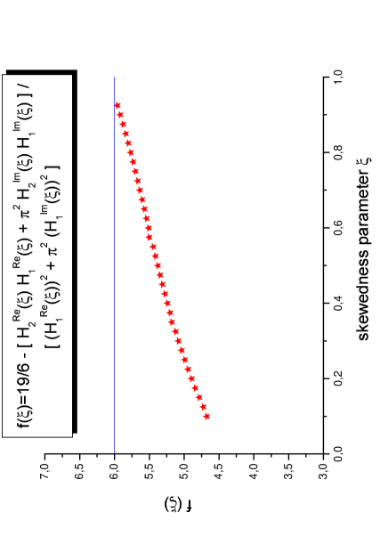
Figure 3: The $\rho$ meson production (quark contribution only): the BLM scales extracted from the squared amplitude.

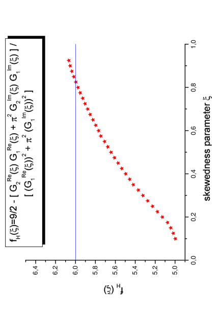
Figure 4: The hybrid meson production: the BLM scales extracted from the squared amplitude.

In this section, we will now extract the corresponding BLM scales working with the squared amplitudes or, in other words, with the cross section. In this case, the BLM equation will be rewritten in the following form:

$$\alpha_{S}^{3}(\mu^{2}_{0})\,\frac{\beta_{0}}{4\pi}\,{\rm ln}\frac{\mu^{2}}{\mu^{2}_{0}}\,|{\cal A}^{{\rm LO}}|^{2}-\alpha_{S}^{3}(\mu^{2}_{0})\,\frac{\beta_{0}}{4\pi}\Biggl{\{}\Re e{\cal A}^{{\rm LO}}\,\Re e{\cal A}^{{\rm NLO},(\beta)}+\Im m{\cal A}^{{\rm LO}}\,\Im m{\cal A}^{{\rm NLO},(\beta)}\Biggr{\}}=0,$$

where we introduced the notations

$${\cal A}^{{\rm NLO},(\beta)}=\biggl{[}C-{\rm ln}\frac{Q^{2}}{\mu^{2}}\biggr{]}\,{\cal A}^{{\rm LO}}+\tilde{\cal A}^{{\rm NLO},(\beta)}.$$ (24)

From (Extraction of the BLM scale from the cross section), we can obtain for the $\rho$ meson function $f^{\rho}(\xi)$ and for the hybrid meson function $f^{H}(\xi)$ the following expressions:

$$f^{\rho}(\xi)=\frac{19}{6}-\frac{H^{Re}_{2}(\xi)H^{Re}_{1}(\xi)+\pi^{2}H^{Im}_{2}(\xi)H^{Im}_{1}(\xi)}{(H^{Re}_{1}(\xi))^{2}+\pi^{2}(H^{Im}_{1}(\xi))^{2}}$$ (25)

and

$$f^{H}(\xi)=\frac{9}{2}-\frac{G^{Re}_{2}(\xi)G^{Re}_{1}(\xi)+\pi^{2}G^{Im}_{2}(\xi)G^{Im}_{1}(\xi)}{(G^{Re}_{1}(\xi))^{2}+\pi^{2}(G^{Im}_{1}(\xi))^{2}}.$$ (26)

In (25) and (26), the structure functions $H^{Re}_{i}(\xi)$, $H^{Im}_{i}(\xi)$, $G^{Re}_{i}(\xi)$ and $G^{Im}_{i}(\xi)$ are the same as they were defined for the BLM scales (18) – (21). The curves of (25) and (26) are shown on Fig. 3 and 4.

Conclusions

We have shown that the usual way of applying the BLM method to the scattering amplitude of exclusive vector meson electroproduction leads to equations fixing the BLM scale which are singular; we believe that this invalidates their straightforward use. The reason that this problem has not been taken care of in previous studies [13] comes from the fact that these studies mostly concentrated on the simpler case of the meson form factor and of amplitudes which were rewritten in terms of this quantity. Let us stress that the singular behaviour of the equations is not specific to QCD. Indeed a simple calculation shows that the same behaviour would be obtained in a QED calculation where gluons are replaced by photons, quarks by electrons, and the $\rho$ meson by a positronium bound state described by a conveniently defined distribution amplitude. We know that it is often advocated that the BLM procedure is easier to understand in the abelian case than in the non-abelian one, but its application to an exclusive process where the amplitude contains both a real and imaginary parts nevertheless suffers from the problem outlined in this paper. We have demonstrated that such singularities do not appear if the BLM procedure is applied to the square of the scattering amplitude, which is a quantity more closely related to an observable, the cross section, rather than the scattering amplitude itself. The phenomenological consequences for the vector meson electroproduction based on this new way of fixing of the BLM scale is studied in [11].

Appendix: Typical functions for the determination of BLM scales

The typical functions in terms of which the renormalization scales corresponding to the $\rho$ and hybrid mesons are rewritten read

$$H^{Re}_{2}(\xi) = {\cal P}\int\limits_{-1}^{1}dxH^{p}_{\rho^{0}}(x,\xi,t_{min})\Biggl{[}{\rm ln}\biggl{|}\frac{\xi+x}{2\xi}\biggr{|}\frac{1}{\xi+x}-{\rm ln}\biggl{|}\frac{\xi-x}{2\xi}\biggr{|}\frac{1}{\xi-x}\Biggr{]}+$$ (27)

$$\frac{\pi^{2}}{2}\biggl{[}H^{p}_{\rho^{0}}(-\xi,\xi,t_{min})-H^{p}_{\rho^{0}}(\xi,\xi,t_{min})\biggr{]};$$

$$H^{Re}_{1}(\xi) = {\cal P}\int\limits_{-1}^{1}dxH^{p}_{\rho^{0}}(x,\xi,t_{min})\Biggl{[}\frac{1}{\xi+x}-\frac{1}{\xi-x}\Biggr{]},$$ (28)

and

$$H^{Im}_{2}(\xi) = \int\limits_{\xi}^{1}dx\frac{H^{p}_{\rho^{0}}(x,\xi,t_{min})-H^{p}_{\rho^{0}}(\xi,\xi,t_{min})}{\xi-x}-$$ (29)

$$\int\limits_{-1}^{-\xi}dx\frac{H^{p}_{\rho^{0}}(x,\xi,t_{min})-H^{p}_{\rho^{0}}(-\xi,\xi,t_{min})}{\xi+x}$$

$$+{\rm ln}\biggl{|}\frac{1-\xi}{2\xi}\biggr{|}\biggl{[}H^{p}_{\rho^{0}}(-\xi,\xi,t_{min})-H^{p}_{\rho^{0}}(\xi,\xi,t_{min})\biggr{]};$$

$$H^{Im}_{1}(\xi) = \biggl{[}H^{p}_{\rho^{0}}(-\xi,\xi,t_{min})-H^{p}_{\rho^{0}}(\xi,\xi,t_{min})\biggr{]}$$ (30)

for the $\rho$ meson production, and

$$G^{Re}_{2}(\xi) = {\cal P}\int\limits_{-1}^{1}dxH^{p}_{H}(x,\xi,t_{min})\Biggl{[}{\rm ln}\biggl{|}\frac{\xi+x}{2\xi}\biggr{|}\frac{1}{\xi+x}+{\rm ln}\biggl{|}\frac{\xi-x}{2\xi}\biggr{|}\frac{1}{\xi-x}\Biggr{]}+$$ (31)

$$\frac{\pi^{2}}{2}\biggl{[}H^{p}_{H}(-\xi,\xi,t_{min})+H^{p}_{H}(\xi,\xi,t_{min})\biggr{]};$$

$$G^{Re}_{1}(\xi) = {\cal P}\int\limits_{-1}^{1}dxH^{p}_{H}(x,\xi,t_{min})\Biggl{[}\frac{1}{\xi+x}+\frac{1}{\xi-x}\Biggr{]},$$ (32)

and

$$G^{Im}_{2}(\xi) = -\int\limits_{\xi}^{1}dx\frac{H^{p}_{H}(x,\xi,t_{min})-H^{p}_{H}(\xi,\xi,t_{min})}{\xi-x}-$$ (33)

$$\int\limits_{-1}^{-\xi}dx\frac{H^{p}_{H}(x,\xi,t_{min})-H^{p}_{H}(-\xi,\xi,t_{min})}{\xi+x}$$

$$+{\rm ln}\biggl{|}\frac{1-\xi}{2\xi}\biggr{|}\biggl{[}H^{p}_{H}(-\xi,\xi,t_{min})+H^{p}_{H}(\xi,\xi,t_{min})\biggr{]};$$

$$G^{Im}_{1}(\xi) = \biggl{[}H^{p}_{H}(-\xi,\xi,t_{min})+H^{p}_{H}(\xi,\xi,t_{min})\biggr{]}$$ (34)

for the hybrid meson production.

References

- [1] P. M. Stevenson, Phys. Rev. D 23 (1981) 2916; P. M. Stevenson, Phys. Lett. B 100 (1981) 61; G. Grunberg, Phys. Rev. D 29 (1984) 2315.
- [2] S. J. Brodsky, G. P. Lepage and P. B. Mackenzie, Phys. Rev. D 28 228 (1983) 228.
- [3] A. V. Belitsky and D. Muller, Phys. Lett. B 513 (2001) 349.
- [4] D. Y. Ivanov, L. Szymanowski and G. Krasnikov, JETP Lett. 80 (2004) 226 [Pisma Zh. Eksp. Teor. Fiz. 80 (2004) 255] [arXiv:hep-ph/0407207].
- [5] A. V. Radyushkin, Fiz. Elem. Chast. Atom. Yadra 20 (1989) 97; R. D. Field, R. Gupta, S. Otto and L. Chang, Nucl. Phys. B 186 (1981) 429; F. M. Dittes and A. V. Radyushkin, Sov. J. Nucl. Phys. 34 (1981) 293 [Yad. Fiz. 34 (1981) 529].
- [6] J. C. Collins, L. Frankfurt and M. Strikman, Phys. Rev. D 56 (1997) 2982 [arXiv:hep-ph/9611433].
- [7] A. V. Radyushkin, Fiz. Elem. Chast. Atom. Yadra 20 (1989) 97.
- [8] I. V. Anikin, B. Pire, L. Szymanowski, O. V. Teryaev and S. Wallon, Phys. Rev. D 70 (2004) 011501
- [9] A. V. Radyushkin, Phys. Rev. D 59 (1999) 014030.
- [10] A. D. Martin, R. G. Roberts, W. J. Stirling and R. S. Thorne, Eur. Phys. J. C 4 (1998) 463 [arXiv:hep-ph/9803445].
- [11] I. V. Anikin, B. Pire, L. Szymanowski, O. V. Teryaev and S. Wallon, Phys. Rev. D 71 (2005) 034021 [arXiv:hep-ph/0411407].
- [12] M. V. Polyakov and C. Weiss, Phys. Rev. D 60 (1999) 114017; B. Lehmann-Dronke, A. Schäfer, M. V. Polyakov and K. Goeke, Phys. Rev. D 63 (2001) 114001.
- [13] S. J. Brodsky, C. R. Ji, A. Pang and D. G. Robertson, Phys. Rev. D 57 (1998) 245 [arXiv:hep-ph/9705221].