1 Introduction

Within quantum chromodynamics, hadrons are described in terms of quarks, anti-quarks and gluons. The usual, well-known, mesons are supposed to contain quarks and anti-quarks as valence degrees of freedom while gluons play the role of carrier of interaction, i.e. they remain hidden in a background. On the other hand, QCD does not prohibit the existence of the explicit gluonic degree of freedom in the form of a vibrating flux tube, for instance. The states where the $q\bar{q}g$ and $gg$ configurations are dominating, hybrids and glueballs, are of fundamental importance to understand the dynamics of quark confinement and the nonperturbative sector of quantum chromodynamics [1]–[5].

The study of these hadrons outside the constituent quark models, namely exotic hybrids, is the main reason of the present paper. We investigate how hybrid mesons with $J^{PC}=1^{-+}$ may be studied through the so-called hard reactions. We focus on deep exclusive meson electroproduction (see, for instance [6]) which is well described in the framework of the collinear approximation where generalized parton distributions (GPDs) [7] and distribution amplitudes[8] describe the nonperturbative parts of a factorized amplitude [9].

In a previous paper [10] we showed that contrarily to naive expectations, the amplitude for the electroproduction of an isotriplet exotic meson with $J^{PC}=1^{-+}$ may be written in a very similar way as the amplitude for non-exotic vector meson electroproduction. The main observation of our work was that the quark-antiquark correlator on the light cone includes a gluonic component due to gauge invariance and leads to a leading twist hybrid light-cone distribution amplitude. In this paper, we extend our analysis of the electroproduction process and calculate the differential cross section as a function of $Q^{2}$.

We also study the hybrid meson as a resonance in the reaction $e\,p\to e\,p\,(\pi^{0}\eta)$. The first experimental investigation of the hybrid with $J^{PC}=1^{-+}$ as the resonance in $\pi^{-}\eta$ mode was implemented by the Brookhaven collaboration E852 [11]. Present candidates for the hybrid states with $J^{PC}=1^{-+}$ include $\pi_{1}(1400)$ which is mostly seen through its $\pi\eta$ decay and $\pi_{1}(1600)$ which is seen through its $\pi\eta^{\prime}$ and $\pi\rho$ decays [12]. Theoretically these states are objects of intense studies [1], mostly through lattice simulations [5].

2 Hybrid meson production amplitude

We propose to study the exotic hybrid meson by means of its deep exclusive electroproduction, i.e.

$$e(k_{1})\,+\,N(p_{1})\,\to\,e(k_{2})\,+H(p)\,+\,N(p_{2}),$$ (1)

where we will concentrate on the subprocess:

$$\gamma^{*}_{L}(q)\,+\,N(p_{1})\,\to\,H_{L}(p)\,+\,N(p_{2})$$ (2)

when the baryon is scattered at small angle. This process is a hard exclusive reaction due to the transferred momentum $Q^{2}$ is large ( Bjorken regime). Within this regime, a factorization theorem is valid, at the leading twist level, which claims that a partonic subprocess part described in perturbative QCD (pQCD) can be detached from universal soft parts, which are generalized parton distributions and meson distribution amplitudes. Below we will analyze in more details how this factorization theorem applies to the process under study.

In this paper, the main object of our investigation is the isotriplet of mesons with quantum numbers $J^{PC}=1^{-+}$. Such mesons can be named as exotic mesons because they do not exist within the usual quark model. To illustrate the latter we shortly remind the main steps of the description and classification of meson states in the quark model.

2.1 Quark model and spectroscopy

It is well known that in the quark model the hadrons, mesons and baryons, are bound states of quark-antiquark or three-quarks systems. Let us consider the mesons, i.e. the quark-antiquark systems. Their total angular momentum results from the summation of spin $S$ and orbital $L$ angular momenta of quarks. Neglecting a spin-orbital interaction, the quantum numbers $S$ and $L$ may be considered as additional quantum numbers for the classification of hadron states. Therefore, the eigenvalues of the squares of the angular momenta read:

$${\bf J}^{2}=J(J+1)\quad{\bf S}^{2}=S(S+1)\quad{\bf L}^{2}=L(L+1),$$

$${\bf J}={\bf S}+{\bf L},$$ (3)

where the number $L$ may take all positive integer values (including zero). The meson octets correspond to the case where $S=0,\,1$. For given values of $S$ and $L$, the total angular momentum $J$ can take the values

$$J\,=\,S+L,\,S+L-1,\,...\,,\left|S-L\right|.$$ (4)

The values $S$ and $L$ are related to the $C$- and $P$-parity of the quark-antiquark system in the form:

$$C=(-)^{L+S},\quad P=(-)^{L+1}.$$ (5)

Consequently, in the quark model, the quantum numbers $S$, $L$, $J$, $P$, $C$ and the relations between them (4), (5) allow to introduce the following classification of the meson states :

• $S=0,\,L=J$ :

  $$J^{PC}=0^{-+},\,1^{+-},\,2^{-+},\,3^{+-},\,...$$ (6)

• $S=1,\,L=0,\,J=1$ :

  $$J^{PC}=1^{--}$$ (7)

• $S=1,\,L=1,\,J=2,\,1,\,0$ :

  $$J^{PC}=0^{++},\,1^{++},\,2^{++}$$ (8)

• $S=1,\,L=2,\,J=3,\,2,\,1$ :

  $$J^{PC}=1^{--},\,2^{--},\,3^{--}$$ (9)

and so on. From this, one can see the mesons with $J^{PC}=0^{--},\,0^{+-},\,1^{-+},\,...\,,$ are forbidden. However, such mesons may be described beyond the quark model. Indeed, we may add an extra degree of freedom (a gluon, for instance) to get the needed quantum numbers, see for instance [3]. Below we will consider this case in more details.

2.2 Kinematics and leading order amplitude

Figure 1: Typical diagram describing the electroproduction of a meson at lowest order. The grey blobs are non-perturbative matrix elements, namely the meson distribution amplitude and the nucleon generalized parton distribution

Let us fix the kinematics of the deep electroproduction process. We are interested in the scaling regime where the virtuality of the photon $Q^{2}=-q^{2}$ is large and scales with the energy of the process. We denote by $p_{1}$ ($p_{2}$) the momentum of the incoming (outgoing) nucleon, while $p$ is the momentum of the longitudinally polarized hybrid meson of mass $M_{H}$. We construct the average momentum $\overline{P}$ and transferred momentum $\Delta$:

$$\overline{P}=\frac{p_{2}+p_{1}}{2},\quad\Delta=p_{2}-p_{1},\quad\Delta^{2}=t.$$ (10)

It is convenient to introduce the following two light-cone vectors:

$$n^{*}=\Lambda(1,{\bf 0}^{T},1),\quad n=\frac{1}{2\Lambda}(1,{\bf 0}^{T},-1),\quad n^{*}\cdot n=1,$$ (11)

where $\Lambda$ is an arbitrary dimensionful parameter . Then the Sudakov decompositions for all the relevant momenta take the form:

$$\Delta_{\mu}=-2\xi n^{*}_{\mu}+\xi\overline{M}^{2}n_{\mu}+\Delta^{T}_{\mu},\quad\Delta^{T}\cdot n=\Delta^{T}\cdot n^{*}=0,$$

$$\overline{P}_{\mu}=n^{*}_{\mu}+\frac{\overline{M}^{2}}{2}n_{\mu},\quad\overline{P}^{2}=\overline{M}^{2},\quad\xi\leq\frac{\sqrt{-\Delta^{2}}}{2\overline{M}}\leq 1,$$

$$q_{\mu}=-2\tilde{\xi}n^{*}_{\mu}+\frac{Q^{2}}{4\tilde{\xi}}n_{\mu},$$

$$p_{\mu}=q_{\mu}-\Delta_{\mu}=2(\xi-\tilde{\xi})n^{*}_{\mu}+\biggl{(}\frac{Q^{2}}{4\tilde{\xi}}-\xi\overline{M}^{2}\biggr{)}n_{\mu}-\Delta^{T}_{\mu}.$$ (12)

Here, the parameters $\xi$ and $\tilde{\xi}$ are related by

$$M_{H}^{2}=4(\xi-\tilde{\xi})\biggl{(}\frac{Q^{2}}{4\tilde{\xi}}-\xi\overline{M}^{2}\biggr{)}+\Delta_{T}^{2}.$$ (13)

The photon longitudinal polarization vector can be written as

$$\varepsilon_{L\,\mu}=\frac{2\tilde{\xi}}{Q}n^{*}_{\mu}+\frac{Q}{4\tilde{\xi}}n_{\mu},$$ (14)

where the notation $Q=\sqrt{Q^{2}}$ is introduced.

The leading order amplitude for the process (1) corresponding to the diagrams in Fig. 1 is

$${\cal A}=\varepsilon_{L}^{\mu}\int d\eta\,e^{iq\cdot\eta}\langle N(p_{2})\,H(p)|\frac{\delta S}{\delta A_{\mu}(\eta)}|N(p_{1})\rangle,$$ (15)

where the $S$-matrix is given by

$$S=T{\rm exp}\biggl{\{}i\int d^{4}x\biggl{(}{\cal L}_{QCD}(x)+{\cal L}_{QED}(x)\biggr{)}\biggr{\}}.$$ (16)

Applying the factorization theorem, this amplitude can be written at leading twist and when $-t\ll Q^{2}$ as

$${\cal A}=\int\limits_{0}^{1}dz\int\limits_{-1}^{1}dx\,\Phi_{H}(z,\mu^{2},\mu_{R}^{2})\,H(x,z,Q^{2},\mu^{2},\mu^{2}_{R})\,F(x,\mu^{2},\mu_{R}^{2})\equiv\Phi_{H}\,\otimes\,H\,\otimes\,F,$$ (17)

where the parameters $\mu^{2}$ and $\mu^{2}_{R}$ are the factorization and renormalization scales, respectively. Throughout this paper, we will adopt the convention that $\mu=\mu_{R}$ . In Eq.(17), $H$ is the hard part of amplitude which is controlled by perturbative QCD. The hybrid meson distribution amplitude $\Phi_{H}$ describes the transition from the partons to the meson, and $F$ denotes generalized parton distributions which are related to nonperturbative matrix elements of bilocal operators between different hadronic states.

More precisely, the factorized amplitude (17) may be written as :

$${\cal A}_{(q)}=\frac{e\pi\alpha_{s}f_{H}C_{F}}{\sqrt{2}N_{c}Q}\biggl{[}e_{u}{\cal H}_{uu}^{-}-e_{d}{\cal H}_{dd}^{-}\biggr{]}{\cal V}^{(H,\,-)},$$ (18)

where

$${\cal H}_{ff}^{\pm} = \int\limits_{-1}^{1}dx\biggl{[}\overline{U}(p_{2})\hat{n}U(p_{1})H_{ff^{\prime}}(x)+\overline{U}(p_{2})\frac{i\sigma_{\mu\alpha}n^{\mu}\Delta^{\alpha}}{2M}U(p_{1})E_{ff^{\prime}}(x)\biggr{]}$$

$$\biggl{[}\frac{1}{x+\xi-i\epsilon}\pm\frac{1}{x-\xi+i\epsilon}\biggr{]},$$

$${\cal V}^{(M,\,\pm)} = \int\limits_{0}^{1}dy\phi^{M}(y)\biggl{[}\frac{1}{y}\pm\frac{1}{1-y}\biggr{]}.$$ (19)

Here, functions $H$ and $E$ are standard leading twist GPD’s and their properties are fairly well-known (see, for instance, a review of Diehl in [7]). In (2.2), we include the definition of ${\cal H}_{ff}^{+}$ and ${\cal V}^{(M,\,+)}$ which will be useful for the comparison with the $\rho$ meson case. The hybrid meson distribution amplitude which enters Eqn. (19) is a new object and we will carefully study it in the next subsection. Note that the simple pole over $y$ in (18) does not lead to any infrared divergency if the function $\phi^{H}(y)$ vanishes when the fraction $y$ goes to zero or unity.

2.3 Hybrid meson distribution amplitude

In this subsection, we will consider in detail the properties of the hybrid meson distribution amplitude (see also [10]). The Fourier transform of the hybrid meson –to–vacuum matrix element of the bilocal vector quark operator may be written as

$$\langle H(p,\lambda)|\bar{\psi}(-z/2)\gamma_{\mu}[-z/2;z/2]\psi(z/2)|0\rangle=$$ (20)

$$if_{H}M_{H}\biggl{[}\biggl{(}e_{\mu}^{(\lambda)}-p_{\mu}\frac{e^{(\lambda)}\cdot z}{p\cdot z}\biggr{)}\int\limits_{0}^{1}dye^{i(\bar{y}-y)p\cdot z/2}\phi^{H}_{T}(y)+p_{\mu}\frac{e^{(\lambda)}\cdot z}{p\cdot z}\int\limits_{0}^{1}dye^{i(\bar{y}-y)p\cdot z/2}\phi^{H}_{L}(y)\biggr{]},$$

where $e^{(\lambda)}$ with $\lambda=(0,\,+1,\,-1)$ describes the polarization states of the hybrid meson. It is convenient to define the four-vector $e^{(0)}_{L}$ corresponding in the ultrarelativistic limit to the longitudinal polarization as

$$e^{(0)}_{L\,\mu}=\frac{e^{(0)}\cdot z}{p\cdot z}p_{\mu}.$$ (21)

For the longitudinal polarization case, only the term with $\phi^{H}_{L}$ contributes, so that

$$\langle H_{L}(p,0)|\bar{\psi}(-z/2)\gamma_{\mu}[-z/2;z/2]\psi(z/2)|0\rangle=if_{H}M_{H}e^{(0)}_{L\,\mu}\int\limits_{0}^{1}dye^{i(\bar{y}-y)p\cdot z/2}\phi^{H}_{L}(y)$$ (22)

where $\bar{y}=1-y$ and $H$ denotes the isovector triplet of hybrid mesons; $f_{H}$ denotes a dimensionful coupling constant of the hybrid meson, so that $\phi^{H}$ is dimensionless. We will discuss its normalization later.

In (2.3) and (22), we insert the path-ordered gluonic exponential along the straight line connecting the initial and final points $[z_{1};z_{2}]$ which provides the gauge invariance for bilocal operator and equals unity in a light-like (axial) gauge. For simplicity of notation we shall omit the index $L$ from the hybrid meson distribution amplitude.

Although exotic quantum numbers like $J^{PC}=1^{-+}$ are forbidden in the quark model, it does not prevent the leading twist correlation function from being non zero. The basis of the argument is that the non-locality of the quark correlator opens the possibility of getting such a hybrid state, because of dynamical gluonic degrees of freedom arising from the Wilson line. This may be seen easily through a Taylor expansion of the non-local correlator

$$\langle H(p,0)|\bar{\psi}(-z/2)\gamma_{\mu}[-z/2;z/2]\psi(z/2)|0\rangle=$$ (23)

$$\sum_{n\,odd}\frac{1}{n!}z_{\mu_{1}}..z_{\mu_{n}}\langle H(p,0)|\bar{\psi}(0)\gamma_{\mu}\stackrel{{\scriptstyle\leftrightarrow}}{{D}}_{\mu_{1}}..\stackrel{{\scriptstyle\leftrightarrow}}{{D}}_{\mu_{n}}\psi(0)|0\rangle,$$

where $D_{\mu}$ is the usual covariant derivative and $\stackrel{{\scriptstyle\leftrightarrow}}{{D_{\mu}}}=\frac{1}{2}(\stackrel{{\scriptstyle\rightarrow}}{{D_{\mu}}}-\stackrel{{\scriptstyle\leftarrow}}{{D_{\mu}}}$). The term corresponding to $z=0$ refers to the standard quark model contribution, which is zero for the exotic hybrid quantum numbers. The first non zero contribution arises from the first derivative contribution in this expansion, and one can check that, more generally, only odd terms contribute in this expansion. It is clear that due to gauge invariance, such occurrence of operators $\stackrel{{\scriptstyle\leftrightarrow}}{{D_{\mu}}}$ naturally provides gluonic degrees of freedom, which enables the production of hybrid state at twist 2 level. One can check explicitly that the corresponding quantum numbers are indeed the one of the hybrid state (see detailed discussion in [10]). Using charge conjugation invariance of $H^{0},$ one can show that the corresponding distribution amplitude is antisymmetric, namely

$$\phi^{H}(y)=-\phi^{H}(1-y)\,.$$ (24)

The result of this analysis is that the hybrid light-cone distribution amplitude is a leading twist quantity which should have a vanishing first moment because of the antisymmetry property of the distribution amplitude. This distribution amplitude obeys usual non-singlet evolution equations [8] and has an asymptotic limit [15]

$$\Phi^{H}=30y(1-y)(1-2y)$$ (25)

The normalization factor (coupling constant) $f_{H}$ is defined through the matrix element of the energy-momentum tensor [16]. It may be related, by making use of the equations of motion, to the matrix element of quark-gluon operator and estimated with the help of the techniques of QCD sum-rules [17]. One of the solutions corresponds to a resonance with mass around $1.4\,{\rm GeV}$ and normalization factor

$$f_{H}\sim 50MeV\,.$$ (26)

If it turns out that only one resonance can be attributed to such an hybrid state, this QCD sum-rule analysis is sufficient to fix the value of $f_{H}.$ If the scenario with two resonances is confirmed, this value of $f_{H}$ corresponds to an effective coupling to the total contribution of these two resonances. Despite the fact that QCD sum rules cannot distinguish at the level of the coupling between two very close resonances and a single one, if one would define $f_{1}$ (resp. $f_{2}$) the coupling to the first resonance (resp. second), one should write

$$f_{H}^{2}=f_{1}^{2}+f_{2}^{2}\,.$$ (27)

Thus, when selecting experimentally each resonance by their decay modes, we know for sure that one of the coupling should be larger than $f_{H}/\sqrt{2}.$ Thus, the fact that the exotic hybrid quantum numbers could be attributed to two very close resonances does not spoil the conclusion about the expected order of magnitude of the hybrid distribution amplitude. From now on, we will consider the case where only one of the $\pi_{1}$ candidates is an exotic hybrid meson.

The coupling constant $f_{H}$ is the subject of evolution given by the formula, see e.g. [18]

$$f_{H}(Q^{2})=f_{H}\left(\frac{\alpha_{S}(Q^{2})}{\alpha_{S}(M_{H}^{2})}\right)^{K_{0}}\;\;\;\;K_{0}=\frac{2\,\gamma_{QQ}(0)}{\beta_{0}}\;,$$ (28)

where the anomalous dimension $\gamma_{QQ}(0)=16/9$ and $\beta_{0}=11-2n_{f}/3$. The exponent $K_{0}$ is thus a small positive number which drives slowly to zero the coupling constant $f_{H}(Q^{2})$. Since experiments are likely to be feasible at moderate values of $Q^{2}$, we neglect this evolution.

3 Cross-sections for hybrid meson electroproduction

In this section, we focus on the computation and analysis of the differential cross section for longitudinally polarized hybrid meson electroproduction. The experimentally accessible differential cross section corresponds to the process (1) for which the reaction (2) is the subprocess. We assume that the virtual photon has a longitudinal polarization, so that the factorization theorem is valid owing to the absence of infrared divergences. We restrict ourselves to the leading twist contributions.

When we estimate hybrid meson electroproduction cross section, we systematically compare it with the similar contribution (i.e. without gluon GPDs) to the cross section for longitudinally polarized $\rho$ meson electroproduction. The unpolarized cross section corresponding to the reaction (2) is defined by

$$\frac{d\sigma_{L}}{d\hat{t}}=\frac{1}{16\pi(\hat{s}-m_{N}^{2})\lambda(\hat{s},-Q^{2},m_{N}^{2})}\frac{1}{2}\sum_{pol.}|{\cal A}_{(q)}|^{2},$$ (29)

where the amplitude ${\cal A}_{(q)}$ is determined by (18); $\hat{s}$, $\hat{t}$ are the usual Mandelstam variables and $m_{N}$ is the nucleon mass. The function $\lambda$ is standardly defined by

$$\lambda^{2}(x,y,z)=x^{2}+y^{2}+z^{2}-2xy-2xz-2yz.$$ (30)

To calculate the cross section (29), we need to model the corresponding GPD’s. We apply the Radyushkin model [27] where the function $H$, see (18), is expressed with the help of double distributions $F^{q}(x,y;t)$. We have

$$H^{q}(x,\xi,t) = \frac{\theta(\xi+x)}{1+\xi}\int\limits_{0}^{{\rm min}\{\frac{x+\xi}{2\xi},\frac{1-x}{1-\xi}\}}dy\,F^{q}\biggl{(}\frac{x+\xi-2\xi y}{1+\xi},y,t\biggr{)}-$$ (31)

$$\frac{\theta(\xi-x)}{1+\xi}\int\limits_{0}^{{\rm min}\{\frac{\xi-x}{2\xi},\frac{1+x}{1-\xi}\}}dy\,F^{\bar{q}}\biggl{(}\frac{\xi-x-2\xi y}{1+\xi},y,t\biggr{)}.$$

where standard notations are used. For the double distribution $F^{q}(X,Y;t)$, we assume the ansatz suggested by Radyushkin [27]:

$$F^{q}(X,Y;t)=\frac{F_{1}^{q}(t)}{F_{1}^{q}(0)}\,q(X)\,6\frac{Y(1-X-Y)}{(1-X)^{3}},$$ (32)

and a similar expression for the anti-quark contribution. As shown in [28], this definition of the double distribution is not completely compatible with the structure of the corresponding matrix elements; introducing D-terms restores the self-consistency of this representation. Taking into account these D-terms, the GPD’s (31) are modified into :

$$H^{q}_{D}(x,\xi,t)=H^{q}(x,\xi,t)+\theta(\xi-|x|)\frac{D(x/\xi,t)}{N_{f}},$$ (33)

where $D(x/\xi,0)$ is given as in [34]. In the present paper, we concentrate on the region where the values of the skewedness parameter $\xi$ are rather small. Hence, it is legitimate to neglect these D-terms in the amplitude of $\rho$ meson production. Meanwhile their contributions to the hybrid meson production always vanish owing to the anti-symmetric properties of these D-terms.

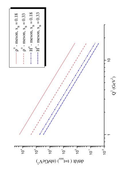
Figure 2: Differential cross section for $\rho$ and hybrid meson production with the naive choice of the renormalization scale and different $x_{B}$.

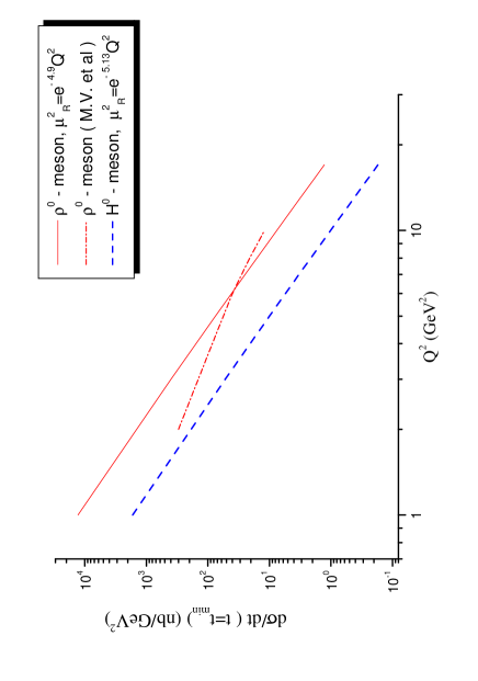
Figure 3: Differential cross-section for exotic hybrid meson electroproduction (dashed line) with $\mu_{R}^{2}=e^{-5.13}Q^{2}$ compared with the quark contribution to $\rho^{0}$ electroproduction (solid line) with $\mu_{R}^{2}=e^{-4.9}Q^{2}$, as a function of $Q^{2},$ for $x_{B}\approx 0.33$. The dash-dotted line is the result of Vanderhaegen et al [26] for $\rho$ electroproduction.

In (32), functions $q(x)$ and $\bar{q}(x)$ are the ordinary quark and anti-quark distributions in the nucleon for which we use the MRST98 parameterization [29]. An important aspect of each model of GPD’s is its dependence ot $t$ [30]. Here it is assumed to be factorizable through the functions $F_{1}^{q}(t)$ for each flavour, which are equal to

$$F_{1}^{u}=2F_{1}^{p}+F_{1}^{n},\quad F_{1}^{d}=2F_{1}^{n}+F_{1}^{p},$$ (34)

where $F_{1}^{p}$ and $F_{1}^{n}$ are the proton and neutron electromagnetic form factors. Note that we neglected the strange form factor because it is small. In the same way, we can write the expression for the function $E$. We neglect here its contribution because it is small and quite model-dependent.

Finally, to get prediction for the cross sections we need to fix the renormalization scales. In order to estimate theoretical uncertainties of this procedure we fix the scale $\mu_{R}^{2}$ in two different ways: firstly, in the naive way, by assuming $\mu^{2}_{R}=Q^{2}$, and secondly, by applying the BLM prescription [22].

The resulting differential cross sections for hybrid meson and $\rho$ meson (quark contribution only) production are shown on Fig. 2 for $x_{B}=0.18$ and $0.33$, using the above mentioned naive scale fixing.

The BLM procedure, which is discussed in details in [42], leads to the following values of the renormalization scales:

$$\mu^{2}_{R}=e^{-4.9}Q^{2},\quad\mbox{for\,\, $\rho$ \,\,meson},$$

$$\mu^{2}_{R}=e^{-5.13}Q^{2},\quad\mbox{for\,\, $H$\,\, meson.}$$ (35)

for the case $\xi=0.2$ (or $x_{B}\approx 0.33$), and

$$\mu^{2}_{R}=e^{-4.68}Q^{2},\quad\mbox{for\,\, $\rho$ \,\,meson},$$

$$\mu^{2}_{R}=e^{-5.0}Q^{2},\quad\mbox{for\,\, $H$\,\, meson.}$$ (36)

for the case $\xi=0.1$ (or $x_{B}\approx 0.18$).

Note that, taking into account the D-terms, the $\rho$ meson BLM scale is slightly diminished. For instance, in the case $x_{B}\approx 0.33$ we have

$$\mu^{2}_{R}=\,e^{-5.4}\,Q^{2}.$$ (37)

These renormalization scales have rather small magnitudes. This has a tendency to enlarge the cross sections but may endanger the validity of the perturbative approach. However, it is possible that the coupling constant $\alpha_{S}$ stays below unity and the perturbative theory does not suffer from the IR divergencies. We will use the Shirkov and Solovtsov’s ansatz [25] where the analytic running coupling constant takes the form:

$$\alpha_{S}^{an}(\mu_{R}^{2})=\frac{4\pi}{\beta_{0}}\biggl{[}\frac{1}{{\rm ln}\mu_{R}^{2}/\Lambda_{QCD}^{2}}+\frac{\Lambda_{QCD}^{2}}{\Lambda_{QCD}^{2}-\mu^{2}_{R}}\biggr{]}.$$ (38)

Here $\Lambda_{QCD}$ is the standard scale parameter in QCD. The second term in (38) assures the absence of a ghost pole at $\mu_{R}^{2}=\Lambda_{QCD}^{2}$ and has a nonperturbative source. Detailed discussion on this point may be found in [23] and references therein.

Recently, in [26] the role of power corrections due to the intrinsic transverse momentum of partons (the kinematical higher twist) has been investigated. In that approach the inclusion of the intrinsic transverse momentum dependence results in a rather strong effect on the differential cross-section before the scaling regime is achieved. In [26], the renormalization scale $\mu^{2}_{R}$ is defined by the gluon virtuality so that the scale is a function of parton fractions flowing into the corresponding gluon propagator.

On Fig. 3, we present our results for the differential cross section of the hybrid meson electroproduction compared to the $\rho$ meson electroproduction, using the BLM scales. We can see that the hybrid cross section is rather sizeable in comparison with the corresponding $\rho$ meson cross section. We also show the results obtained in [26] for the $\rho$ meson electroproduction. We see that in the region $Q^{2}\sim 5-10\,{\rm GeV}^{2}$ the size of the $\rho$ meson cross section obtained with the inclusion of transverse momentum effects is very close to the analogous cross section computed with the BLM scale and without the intrinsic transverse momentum dependence. On the other hand, for higher values of $Q^{2}$ the leading order amplitude computed with the BLM scale fixing is falling faster that the corresponding amplitude derived in Ref. [26], whereas for smaller values of $Q^{2}$ it is larger than that prediction. We do not want to claim here that kinematical higher twist contributions have no effects at low values of $Q^{2}$ but rather that a rather strong effect on the $Q^{2}$ dependence of the cross sections may be dictated by another mechanism which is much more controllable since it depends on the estimate of higher order perturbative contributions.

All this shows that the scale fixing ambiguities lead to a non negligible theoretical uncertainty on the absolute value of cross sections. It is important however to understand that most of this uncertainty does not apply to ratios of cross sections, and in particular to the most interesting ratio $d\sigma^{H}\,:\,d\sigma^{\rho}$, which measures the expected cross section for hybrid production with respect to the well measured and large cross section for $\rho$ meson production. Indeed, as shown on Table $1$, this ratio is very insensitive to the scale fixing procedure. Moreover it is not small when $x_{B}$ is large enough and almost $Q^{2}$ independent. The decreasing value of the ratio when $x_{B}$ diminishes comes from the relative sign of the two terms contributing in (18), i.e. when $\xi\to 0$ the structure $\cal{H}^{-}$ goes to zero too.

In conclusion of this section, we would like to stress that the present work has demonstrated the feasibility of hybrid meson production experiments in electroproduction at moderate energies. An obvious remaining question is how much of the cross section is observable in a dedicated experiment. If the experiment is able to detect the final state electron and baryon and to measure their momenta with good accuracy, a missing mass analysis may allow to identify and study all decay channels of the hybrid. In the next sections, we discuss the cases where the hybrid meson is detected through a particular decay channel.

$x_{B}$	$0.33$				$0.18$
$Q^{2}\,({\rm GeV}^{2})$	3.0	7.0	11.0	17.0	3.0	7.0	11.0	17.0
$\mu^{2}_{R}=Q^{2}$	0.123	0.123	0.123	0.123	0.0325	0.0326	0.0326	0.0326
$\mu^{2}_{R}=\mu_{BLM}^{2}$	0.131	0.133	0.133	0.134	0.0356	0.0362	0.0365	0.0367

Table 1: Ratio $d\sigma^{H}:d\sigma^{\rho}$ for both the naive and BLM scales and for the different values of $x_{B}$.

4 Study of hybrid mesons via the electroproduction of $\pi\eta$ pairs

In the case where there is no recoil detector which allows to identify the hybrid production events through a missing mass reconstruction, one will have to base an identification process through the possible decay products of the hybrid meson $H^{0}$. Since the particle $\pi_{1}(1400)$ has a dominant $\pi\eta$ decay mode, we now proceed to the description of the electroproduction process

$$e(k_{1})+N(p_{1})\to e(k_{2})+\pi^{0}(p_{\pi})+\eta(p_{\eta})+N(p_{2})$$ (39)

or

$$\gamma^{*}(q)+N(p_{1})\to\pi^{0}(p_{\pi})+\eta(p_{\eta})+N(p_{2}).$$ (40)

To perform a leading order computation of such process (see Fig. 4). we need to introduce the concept of generalized distribution amplitude (GDA) [31] for $\pi\eta$.

4.1 $\pi\eta$ generalized distribution amplitude

In this subsection, we briefly introduce and discuss the generalized distribution amplitude related to the $\pi\eta$–to–vacuum matrix element. On the basis of Lorentz invariance, the $\pi^{0}\eta$ GDA may be defined as :

$$\langle\pi^{0}(p_{\pi})\eta(p_{\eta})|\bar{\psi}_{f_{2}}(-z/2)\gamma^{\mu}[-z/2;z/2]\tau^{3}_{f_{2}f_{1}}\psi_{f_{1}}(-z)|0\rangle=$$

$$p^{\mu}_{\pi\eta}\int\limits_{0}^{1}dye^{i(\bar{y}-y)p_{\pi\eta}\cdot z/2}\Phi^{(\pi\eta)}(y,\zeta,m_{\pi\eta}^{2}),$$ (41)

where the total momentum of $\pi\eta$ pair is $p_{\pi\eta}=p_{\pi}+p_{\eta}$ while $m^{2}_{\pi\eta}=p^{2}_{\pi\eta}$. We omit the $Q^{2}$ dependence of the $\pi^{0}\eta$ GDA’s which is the same as the one discussed above for the hybrid meson distribution amplitude. Note that the $\pi\eta$ distribution amplitude $\Phi^{(\pi\eta)}$ describes non resonant as well as resonant contributions. It does not possess any symmetry properties concerning the $\zeta$-parameter.

Let us now discuss the $\zeta$ parameter. When the two mesons have equal masses, the parameter $\zeta$ is usually defined as $\zeta=p_{\pi}^{+}/p^{+}$. In the case of two different particles it is more convenient to define the parameter $\tilde{\zeta}$ in the following way:

$$\tilde{\zeta}=\frac{p_{\pi}^{+}}{(p_{\pi}+p_{\eta})^{+}}-\frac{m^{2}_{\pi}-m^{2}_{\eta}}{2m^{2}_{\pi\eta}},$$

$$1-\tilde{\zeta}=\frac{p_{\eta}^{+}}{(p_{\pi}+p_{\eta})^{+}}+\frac{m^{2}_{\pi}-m^{2}_{\eta}}{2m^{2}_{\pi\eta}}.$$ (42)

Then, we get the ordinary relation between $\tilde{\zeta}$ and the angle $\theta_{cm}$, defined as the polar angle of the $\pi$ meson in the center of mass frame of the meson pair:

$$2\tilde{\zeta}-1=\beta\cos\theta_{cm}.$$ (43)

In (43), the standard $\beta$-function is given by

$$\beta=\frac{2|{\bf p}|}{m_{\pi\eta}},$$ (44)

where ${\bf|p|}$ denote the modulus of three-dimension momentum of $\pi$ and $\eta$ mesons in the center–of–mass system.

Figure 4: Typical diagram describing the electroproduction of $\pi\eta$ pair. The higher and lower blobs represent the GDA’s and GPD’s, respectively.

In the reaction under study, the $\pi\eta$ state may have total momentum, parity and charge-conjugation in the following sequence

$$J^{PC}=0^{++},\,1^{-+},\,2^{++},\,...$$

that corresponds to the following values of the $\pi\eta$ orbital angular momentum $L$:

$$L=0,\,1,\,2,\,...$$

respectively. We can see that a resonance with a $\pi\eta$ decay mode for odd orbital angular momentum $L$ should be considered as an exotic meson.

The mass region around $1400$ ${\rm MeV}$ is dominated by the strong $a_{2}(1329)\,(2^{++})$ resonance [32]. It is therefore natural to look for the interference of the amplitudes of hybrid and $a_{2}$ production, which is linear, rather than quadratic in the hybrid electroproduction amplitude. Such interference arises from the usual representation of the $\pi\eta$ generalized distribution amplitude in the form suggested by its asymptotic expression :

$$\Phi^{(\pi\eta),\,a}(y,\tilde{\zeta},m_{\pi\eta}^{2})=10y(1-y)C^{(3/2)}_{1}(2y-1)\sum_{l=0}^{2}B_{1l}(m_{\pi\eta}^{2})P_{l}(\cos\theta).$$ (45)

Keeping only $L=1$ and $L=2$ terms, we model the $\pi\eta$ distribution amplitude in the following form:

$$\Phi^{(\pi\eta)}(y,\zeta,m_{\pi\eta}^{2})=30y(1-y)(2y-1)\biggl{[}\,B_{11}(m_{\pi\eta}^{2})P_{1}(\cos\theta)+B_{12}(m_{\pi\eta}^{2})P_{2}(\cos\theta)\biggr{]},$$ (46)

with the coefficient functions $B_{11}(m_{\pi\eta}^{2})$ and $B_{12}(m_{\pi\eta}^{2})$ related to corresponding Breit-Wigner amplitudes when $m^{2}_{\pi\eta}$ is in the vicinity of $M^{2}_{a_{2}},\,M^{2}_{H}$. We have (see the technical details how to calculate these coefficient functions in Appendix A):

$$B_{11}(m^{2}_{\pi\eta})\biggl{|}_{m^{2}_{\pi\eta}\approx M^{2}_{H}}=\frac{5}{3}\,\frac{g_{H\pi\eta}f_{H}M_{H}\beta}{M^{2}_{H}-m^{2}_{\pi\eta}-i\Gamma_{H}M_{H}}$$ (47)

and

$$B_{12}(m^{2}_{\pi\eta})\biggr{|}_{m^{2}_{\pi\eta}\approx M^{2}_{a_{2}}}=\frac{10}{9}\frac{ig_{a_{2}\pi\eta}f_{a_{2}}M^{2}_{a_{2}}\beta^{2}}{M^{2}_{a_{2}}-m^{2}_{\pi\eta}-i\Gamma_{a_{2}}M_{a_{2}}}.$$ (48)

In the $a_{2}$ case, we use the results and conventions of [33]; note that the coupling constant $g_{a_{2}\pi\eta}$ has mass dimension equal to $-1$.

The coupling constants $g_{H\pi\eta}$ and $g_{a_{2}\pi\eta}$ may be estimated through the approximate measurements of the partial widths of the $a_{2}$ and hybrid meson in the $\pi\eta$ decay channel, we have:

$$\Gamma(H\to\pi\eta)=\frac{1}{16\pi}g^{2}_{H\pi\eta}\frac{\lambda^{3}(M^{2}_{H},m^{2}_{\pi},m^{2}_{\eta})}{M^{5}_{H}},$$

$$\Gamma(a_{2}\to\pi\eta)=\frac{1}{24\pi}g^{2}_{a_{2}\pi\eta}\frac{\lambda^{5}(M^{2}_{a_{2}},m^{2}_{\pi},m^{2}_{\eta})}{M^{7}_{a_{2}}}.$$ (49)

Neglecting the masses of $\pi$ and $\eta$ mesons compared to the $a_{2}$ and hybrid meson masses, we get

$$g^{2}_{H\pi\eta}\approx\frac{16\pi}{M_{H}}\Gamma(H\to\pi\eta),\quad g^{2}_{a_{2}\pi\eta}\approx\frac{24\pi}{M_{a_{2}}^{3}}\Gamma(a_{2}\to\pi\eta).$$ (50)

4.2 Differential cross section for $\pi\eta$ electroproduction

Figure 5: Typical process describing the electroproduction of a $\pi\eta$ pair.

Let us first fix the kinematics. For reaction (39) we choose:

$$k_{1}=(\varepsilon_{1},\,\varepsilon_{1}\sin\theta_{1},\,0,\,\varepsilon_{1}\cos\theta_{1})$$

$$p_{1}=(E_{1},\,0,\,0,\,p^{3}_{1}),\quad q=k_{1}-k_{2}=(q_{0},\,0,\,0,\,-p^{3}_{1}),$$

$$p_{2}=(E_{2},\,|{\bf p}_{2}|\cos\phi\sin\theta,\,|{\bf p}_{2}|\sin\phi\sin\theta,\,|{\bf p}_{2}|\cos\theta).$$ (51)

The following Mandelstam and dimensionless variables can be defined as (here, the ”hatted” symbols refer to the subprocess (40))

$$\hat{s}=(p_{\pi\eta}+p_{2})^{2}=(q+p_{1})^{2},\quad\hat{t}=(p_{2}-p_{1})^{2},\quad S=(k_{1}+p_{1})^{2},$$ (52)

and

$$x_{B}=\frac{Q^{2}}{2p_{1}\cdot q},\quad y_{l}=\frac{p_{1}\cdot q}{p_{1}\cdot k_{1}}.$$ (53)

In (4.2), the energies and momenta can be expressed as

$$\varepsilon_{1}=\frac{S-m_{N}^{2}-Q^{2}}{2\sqrt{\hat{s}}},\quad\varepsilon_{2}=\frac{S-\hat{s}}{2\sqrt{\hat{s}}},$$

$$E_{1}=\frac{\hat{s}+m^{2}_{N}+Q^{2}}{2\sqrt{\hat{s}}},\quad E_{2}=\frac{\hat{s}-m^{2}_{\pi\eta}+m^{2}_{N}}{2\sqrt{\hat{s}}},\quad q_{0}=\frac{\hat{s}-m^{2}_{N}-Q^{2}}{2\sqrt{\hat{s}}},$$

$$|{\bf q}|=|{\bf p}_{1}|=\frac{\lambda(\hat{s},m^{2}_{N},-Q^{2})}{2\sqrt{\hat{s}}},\quad|{\bf p}_{\pi\eta}|=|{\bf p}_{2}|=\frac{\lambda(\hat{s},m^{2}_{\pi\eta},m^{2}_{N})}{2\sqrt{\hat{s}}},$$ (54)

where the kinematical function $\lambda$ in defined in (30).

The corresponding angles take the forms

$$\cos\theta_{2}=\frac{2Q^{2}\hat{s}}{(S-\hat{s})\lambda(\hat{s},m^{2}_{N},-Q^{2})}-\frac{\hat{s}-m^{2}_{N}-Q^{2}}{\lambda(\hat{s},m^{2}_{N},-Q^{2})},$$

$$\cos\theta=\frac{2\hat{s}(\hat{t}-2m^{2}_{N})+(\hat{s}+m^{2}_{N}+Q^{2})(\hat{s}-m^{2}_{\pi\eta}+m^{2}_{N})}{\lambda(\hat{s},m^{2}_{N},-Q^{2})\lambda(\hat{s},m^{2}_{\pi\eta},m^{2}_{N})}.$$ (55)

It is useful to note the following relations between the invariants:

$$x_{B}=\frac{Q^{2}}{\hat{s}+Q^{2}-m^{2}_{N}},\quad y_{l}=\frac{Q^{2}}{x_{B}(S-m^{2}_{N})}=\frac{\hat{s}+Q^{2}-m^{2}_{N}}{S-m^{2}_{N}},$$

$$Q^{2}=x_{B}y_{l}(S-m^{2}_{N}),\quad\hat{s}=\frac{1-x_{B}}{x_{B}}Q^{2}+m^{2}_{N}.$$ (56)

One may also work within the center-of-mass system of the meson pair, where we have after the corresponding boost,

$$p_{\pi}=(E_{\pi},\,|{\bf p}|\sin\theta_{cm},\,0,\,|{\bf p}|\cos\theta_{cm}),\quad p_{\eta}=(E_{\eta},\,-|{\bf p}|\sin\theta_{cm},\,0,\,-|{\bf p}|\cos\theta_{cm}),$$ (57)

where the energies and momenta of the mesons take the forms

$$E_{\pi}=\frac{m^{2}_{\pi\eta}-m^{2}_{\eta}+m^{2}_{\pi}}{2m_{\pi\eta}},\quad E_{\eta}=\frac{m^{2}_{\pi\eta}-m^{2}_{\pi}+m^{2}_{\eta}}{2m_{\pi\eta}},\quad|{\bf p}|=\frac{\lambda(m^{2}_{\pi\eta},m^{2}_{\eta},m^{2}_{\pi})}{2m_{\pi\eta}}.$$ (58)

We now come to the expression for the differential cross section of reaction (39). The amplitude of this reaction is given by

$$T^{\pi^{0}\eta}=\bar{u}(k_{2},s_{2})\gamma\cdot\varepsilon_{L}u(k_{1},s_{1})\frac{1}{q^{2}}{\cal A}_{(q)}^{\pi^{0}\eta},$$ (59)

leading, keeping the leading order in $Q^{2}$, to

$$|T^{\pi^{0}\eta}|^{2}=\frac{4e^{2}(1-y_{l})}{Q^{2}y_{l}^{2}}|{\cal A}_{(q)}^{\pi^{0}\eta}|^{2}\,.$$ (60)

The amplitude of subprocess (40) reads

$${\cal A}_{(q)}^{\pi^{0}\eta}=\frac{e\pi\alpha_{s}C_{F}}{N_{c}\,Q}\biggl{[}e_{u}{\cal H}_{uu}-e_{d}{\cal H}_{dd}\biggr{]}$$

$$\biggl{[}B_{11}(m_{\pi\eta}^{2})P_{1}(\cos\theta_{cm})+B_{12}(m_{\pi\eta}^{2})P_{2}(\cos\theta_{cm})\biggr{]}.$$ (61)

Finally, the differential cross section of process (39) takes the form

$$\frac{d\sigma^{\pi^{0}\eta}}{dQ^{2}\,dy_{l}\,d\hat{t}\,dm_{\pi\eta}\,d(\cos\theta_{cm})}=\frac{1}{4(4\pi)^{5}}\,\frac{m_{\pi\eta}\beta}{y_{l}\lambda^{2}(\hat{s},-Q^{2},m^{2}_{N})}\,|T^{\pi^{0}\eta}|^{2}.$$ (62)

5 Calculation of the angular asymmetry

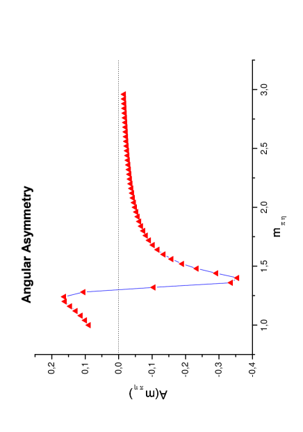
Figure 6: The angular asymmetry as a function of $m_{\pi\eta}$.

Asymmetries are often a good way to get a measurable signal for a small amplitude, by taking profit of its interference with a larger one. In our case, since the hybrid production amplitude may be rather small with respect to a continuous background, we propose to use the supposedly large amplitude for $a_{2}$ electroproduction as a magnifying lens to unravel the presence of the exotic hybrid meson. Since these two amplitudes describe different orbital angular momentum of the $\pi$ and $\eta$ mesons, the asymmetry which is sensitive to their interference is an angular asymmetry defined by

$$A(Q^{2},y_{l},\hat{t},m_{\pi\eta})=\frac{\int\cos\theta_{cm}\,d\sigma^{\pi^{0}\eta}(Q^{2},y_{l},\hat{t},m_{\pi\eta},\cos\theta_{cm})}{\int d\sigma^{\pi^{0}\eta}(Q^{2},y_{l},\hat{t},m_{\pi\eta},\cos\theta_{cm})}$$ (63)

as a weighted integral over polar angle $\theta_{cm}$ of the relative momentum of $\pi$ and $\eta$ mesons. The angle $\theta_{cm}$ is related to the parameter $\tilde{\zeta}$ by formula (43). Due to the fact that the $\cos\theta_{cm}$-independent factors in both the numerator and denominator of (63) are completely factorized and, on the other hand, these factors are the same, we are able to rewrite the asymmetry (63) as

$$A(m_{\pi\eta})=\frac{\int d(\cos\theta_{cm})\,\cos\theta_{cm}\biggl{|}B_{11}(m_{\pi\eta}^{2})P_{1}(\cos\theta_{cm})+B_{12}(m_{\pi\eta}^{2})P_{2}(\cos\theta_{cm})\biggr{|}^{2}}{\int d(\cos\theta_{cm})\,\biggl{|}B_{11}(m_{\pi\eta}^{2})P_{1}(\cos\theta_{cm})+B_{12}(m_{\pi\eta}^{2})P_{2}(\cos\theta_{cm})\biggr{|}^{2}},$$ (64)

and, calculating the $\cos\theta_{cm}$-integral analytically, to obtain

$$A(m_{\pi\eta})=\frac{N(m_{\pi\eta})}{D(m_{\pi\eta})},$$ (65)

with

$$N=\frac{8}{15}\Re\biggl{[}B_{11}(m_{\pi\eta}^{2})B_{12}^{*}(m_{\pi\eta}^{2})\biggr{]},\quad D=\frac{2}{3}\biggl{|}B_{11}(m_{\pi\eta}^{2})\biggr{|}^{2}+\frac{2}{5}\biggl{|}B_{12}(m_{\pi\eta}^{2})\biggr{|}^{2}.$$ (66)

While in the two-pion production case the interference between the isoscalar and isovector channels can be investigated, we here restrict to the interference between $L=1$ and $L=2$ modes of $\pi^{0}\eta$. As a result, the introduction of the so-called intensity density (see [34]), i.e. the integrated-over-invariants value, useful for the two-pion modes, completely coincides with the value (65) for our case.

Our estimation of the asymmetry (65) is shown on Fig. 6. Since the numerator of (65), i.e. the real part of the product of $B_{11}(m_{\pi\eta}^{2})$ and $B_{12}^{*}(m_{\pi\eta}^{2})$, is proportional to the cosine of the phase difference $\Delta\delta_{1,2}=\delta_{l=1}-\delta_{l=2}$ the zeroth value of (65) takes place at $\Delta\delta_{1,2}=\pi/2$. This is achieved for $m_{\pi\eta}\approx 1.3\,{\rm GeV}$. Besides, one can see from Fig. 6 that the first positive extremum is located at $m_{\pi\eta}$ around the mass of $a_{2}$ meson while the second negative extremum corresponds to the hybrid meson mass.

Note that this angular asymmetry is completely similar to the charge asymmetry which was studied in $\pi^{+}\pi^{-}$ electroproduction at HERMES [35].

6 Note on the $\pi\pi\pi$ channel

The hybrid candidate $\pi_{1}(1600)$ has been also seen through a $\pi\pi\pi$ decay channel. In that case the deep exclusive electroproduction of three pions provides the background which should be studied, including the possible interference effects of hybrid meson and the background. The analysis that we have described in section 4 and 5 may be adapted to the three body case by using the results of [36]. At the leading twist level the generalized distribution amplitude of the charge conjugation even state may be written in complete analogy to the pion light-cone distribution from the large distance matrix element

$$S_{\alpha\beta}={P^{+}\over 2\pi}\int\!dx^{-}\,e^{-iy(P^{+}x^{-})}\,\raise-3.0pt\hbox{\scriptsize out}\langle\pi\pi\pi|\,\bar{\psi}_{\alpha}(x^{-}v^{\prime})\psi_{\beta}(0)\,|0\rangle\raise-3.0pt\hbox{\scriptsize in}$$ (67)

as

$$S_{q,\alpha\beta}^{\phantom{\mu}}\,\gamma^{+}_{\alpha\beta}\gamma_{5}=\frac{i}{f_{\pi}}\Phi^{+}_{q}(z,\zeta_{0},\zeta_{+},\zeta_{-};W_{12}^{2},W_{13}^{2},W_{23}^{2},)\,P^{+}.$$ (68)

The three light cone fractions are normalized by the condition $\zeta_{0}+\zeta_{+}+\zeta_{-}=1$, making only two of them independent, while the squared total energy of the three pions is $W^{2}=W_{12}^{2}+W_{13}^{2}+W_{23}^{2}-3m_{\pi}^{2}$, where $W_{ij}$ are the invariant masses of the pairs of mesons.

Charge conjugation invariance provides a symmetry relation:

$$\Phi^{+}(y,\zeta_{0},\zeta_{+},\zeta_{-})=\Phi^{+}(1-y,\zeta_{0},\zeta_{-},\zeta_{+}).$$ (69)

The asymptotic $z$-dependence is just

$$\Phi^{+}_{q}(y,\zeta_{0},\zeta_{+},\zeta_{-})=\frac{1}{6(1+a)}y(1-y)(\zeta_{0}+a\zeta_{0}^{2}),$$ (70)

where $a$ is an unknown parameter and the normalization has been fixed with the help of the fact that putting both charged pion momenta to zero, one should get the GDA equal to the pion distribution amplitude. The QCD evolution is the same as for the pion distribution amplitude, i.e. with a vanishing anomalous dimension.

Conversely, the generalized distribution amplitude $\Phi^{-}(y,\zeta_{0},\zeta_{+},\zeta_{-})$ of the charge conjugation odd state obeys the equation :

$$\Phi^{-}(y,\zeta_{0},\zeta_{+},\zeta_{-})=-\Phi^{-}(1-y,\zeta_{0},\zeta_{-},\zeta_{+}).$$ (71)

and its asymptotic $z$-dependence is

$$\Phi^{-}_{q}(y,\zeta_{0},\zeta_{+},\zeta_{-})\sim y(1-y)(2y-1)P(\zeta_{0},\zeta_{+},\zeta_{-}),$$ (72)

where $P$ is a polynomial of degree 3 with the symmetry property

$$P(\zeta_{0},\zeta_{+},\zeta_{-})=P(\zeta_{0},\zeta_{-},\zeta_{+}).$$

Its QCD evolution is the same as for the hybrid distribution amplitude. The interference with $\pi_{1}(1600)$ may produce an angular asymmetry similar to that of Section 5, although the appearance of third pion makes the analysis more complicated.

7 Diffractive production of the hybrid at large energy

At large energy, one should consider a different framework, namely the impact representation [2] where the meson electroproduction amplitude is factorized in impact factors and a reggeized two or three gluon exchange known as perturbative Pomeron or Odderon exchange. Without performing a detailed phenomenology of this reaction in this regime let us recall some well known formula and briefly propose a strategy to help future (or present) experiments at high energy to search for hybrids.

The even charge conjugation of the hybrid meson selects in this case the Odderon exchange [37] and the amplitude for its electroproduction is equal to

$$\mathcal{M}_{O}=-\frac{8\,\pi^{2}\,s}{3!}\int\,\frac{d^{2}{\bf k}_{1}\,d^{2}{\bf k}_{2}\,d^{2}{\bf k}_{3}\,\delta^{(2)}({\bf k}_{1}+{\bf k}_{2}+{\bf k}_{3}-{\bf p}_{H^{0}})}{(2\pi)^{6}\,{\bf k}_{1}^{2}\,{\bf k}_{2}^{2}\,{\bf k}_{3}^{2}}J_{O}^{\gamma^{*}\rightarrow H^{0}}\cdot J_{O}^{N\rightarrow N^{\prime}}$$ (73)

where $J_{O}^{\gamma^{*}\rightarrow H^{0}}({\bf k}_{1},{\bf k}_{2},{\bf k}_{3})$ and $J_{O}^{N\rightarrow N^{\prime}}({\bf k}_{1},{\bf k}_{2},{\bf k}_{2})$ are the impact factors for the transition $\gamma^{*}\to H^{0}$ via Odderon exchange and of the nucleon in initial state $N$ into the nucleon in the final state $N^{\prime}$. The impact factors are defined as the $s-$channel discontinuities of the corresponding $S-$matrices describing the $\gamma^{*}O\to H^{0}$ and $NO\to N^{\prime}$ processes projected on the longitudinal (nonsense) polarizations of the virtual gluons in the $t-$channel.

The upper impact factors are calculated by the use of standard methods. The leading order calculation in pQCD gives in the case of a longitudinal polarized photon :

$$J_{O}^{\gamma_{L}^{*}}({\bf k}_{1},{\bf k}_{2},{\bf k}_{3})=-\frac{i\,e\,g^{3}\,d^{abc}\,Q}{4\,N_{C}}\;\int\limits_{0}^{1}\,dy\,y{\bar{y}}\,P_{O}({\bf k}_{1},{\bf k}_{2},{\bf k}_{3})\,\frac{1}{3}\Phi^{H^{0}}(y)$$ (74)

where ${\bf k}_{1}+{\bf k}_{2}+{\bf k}_{3}={\bf p}_{H^{0}}$ and

$$P_{O}({\bf k}_{1},{\bf k}_{2},{\bf k}_{3})=\frac{1}{y^{2}{\bf p}_{H^{0}}^{\;2}+\mu^{2}}-\frac{1}{{\bar{y}}^{2}{\bf p}_{H^{0}}^{\;2}+\mu^{2}}$$

$$-\sum\limits_{i=1}^{3}\left(\frac{1}{({\bf k}_{i}-y{\bf p}_{H^{0}})^{2}+\mu^{2}}-\frac{1}{({\bf k}_{i}-{\bar{y}}{\bf p}_{H^{0}})^{2}+\mu^{2}}\right)$$ (75)

The proton impact factor cannot be calculated within perturbation theory. One may use phenomenological eikonal models of these impact factors proposed in Ref [38] which read

$$J_{O}^{N\rightarrow N^{\prime}}=-i\frac{{\bar{g}}^{3}\,d^{abc}}{4\,N_{C}}\,3\left[F({\bf p}_{H^{0}},0,0)-\sum\limits_{i=1}^{3}F({\bf k}_{i},{\bf p}_{H^{0}}-{\bf k}_{i},0)+2\,F({\bf k}_{1},{\bf k}_{2},{\bf k}_{3})\right]$$ (76)

where

$$F({\bf k}_{1},{\bf k}_{2},{\bf k}_{3})=\frac{A^{2}}{A^{2}+\frac{1}{2}\left[({\bf k}_{1}-{\bf k}_{2})^{2}+({\bf k}_{2}-{\bf k}_{3})^{2}+({\bf k}_{3}-{\bf k}_{1})^{2}\right]}$$ (77)

and $A=\frac{m_{\rho}}{2}$. In these equations we denote the soft QCD-coupling constant by ${\bar{g}}$ and one may take ${\alpha}_{soft}=\bar{g}^{2}/(4\pi)=0.5$ as a reasonable mean value.

Since the Odderon amplitude is known to be rather small, producing the hybrid in electroproduction at large energy will be rather difficult. It will thus be useful to search for the hybrid meson in this context through an interference of a Pomeron mediated amplitude to a Odderon mediated one, as discussed in [39]. The three pion channel discussed in the preceeding section is interesting in this respect since a charge asymmetry between the $\pi^{+}$ and the $\pi^{-}$ will single out this interference. The charge asymmetry to measure is defined as a integral weighted with an antisymmetric function in the exchange $\zeta^{+}\to\zeta^{-}$, the simplest example being $\zeta^{+}-\zeta^{-}$. :

$$A(Q^{2},t,m_{3\pi}^{2})=\frac{\int\limits_{0}^{1}\,d\zeta^{+}\,d\zeta^{-}(\zeta^{+}-\zeta^{-})\,2\ \mbox{Re}\left[{\cal M}_{P}^{\gamma^{*}_{L}}({\cal M}_{O}^{\gamma^{*}_{L}})^{*}\right]}{\int\limits_{0}^{1}\,d\zeta^{+}\,d\zeta^{-}\left[|{\cal M}_{P}^{\gamma^{*}_{L}}|^{2}+|{\cal M}_{O}^{\gamma^{*}_{L}}|^{2}\right]}$$ (78)

which is approximately equal to the ratio of the Odderon exchange amplitude and the Pomeron exchange amplitude, which one may approximate to the production of a $J^{PC}=1^{--}$ state like $\omega(1650)$.

This may be related to a forward-backward asymmetry in the rest frame of the two charged pions, the forward direction being defined as the direction of the neutral $\pi^{0}$ meson. Defining the $\theta$ angle as the angle of the $\pi^{+}$ to the $\pi^{0}$ 3-momenta in this frame, one gets

$$A(Q^{2},t,m_{3\pi}^{2})=\frac{\int\cos\theta\,d\sigma(s,Q^{2},t,m_{3\pi}^{2},\theta)}{\int d\sigma(s,Q^{2},t,m_{3\pi}^{2},\theta)}=\frac{2\int\limits_{-1}^{1}\,d(\cos\theta)\,\cos\theta\,\Re\left[{\cal M}_{P}^{\gamma^{*}_{L}}({\cal M}_{O}^{\gamma^{*}_{L}})^{*}\right]}{\int\limits_{-1}^{1}\,d\cos\theta\left[|{\cal M}_{P}^{\gamma^{*}_{L}}|^{2}+|{\cal M}_{O}^{\gamma^{*}_{L}}|^{2}\right]}$$ (79)

8 Conclusion

In conclusion, we have calculated in this paper the leading twist contribution to exotic hybrid meson with $J^{PC}=1^{-+}$ electroproduction amplitude in the deep exclusive region. The resulting order of magnitude is somewhat smaller than the $\rho$ electroproduction but similar to the $\pi$ electroproduction. The obtained cross section is sizeable and should be measurable at dedicated experiments at JLab, Hermes or Compass.

We made a systematic comparison with the non-exotic vector meson production. To take into account NLO corrections, the differential cross-sections for these processes have been computed using the BLM prescription for the renormalization scale. In the case of $\rho$ production, our estimate is not far from a previous one which took into account kinematical higher twist corrections.

We have also discussed in detail the $\pi\eta$ mode corresponding to the $\pi_{1}(1400)$ candidate in the reaction $e\,p\to e\,p\,\pi^{0}\eta$. We have calculated an angular asymmetry implied by charge conjugation properties and got a sizeable hybrid effect which may be experimentally checked.

In the region of small $Q^{2}$ higher twist contributions should be carefully studied and included. Note that they have already been considered in the case of deeply virtual Compton scattering [40] where their presence was dictated by gauge invariance, and for transversely polarized vector mesons [41] where the leading twist component vanishes. We leave this study for future works.

Finally, the diffractive production at very high energy has been briefly studied. The weakness of Odderon mediated processes makes the study of hybrid meson electroproduction a very difficult task for HERA experiments.

9 Acknowledgments

We acknowledge useful discussions with A. Bakulev, I. Balitsky, V. Braun, M. Diehl, G. Korchemsky, C. Michael, S. Mikhailov and O. Pene. This work is supported in part by INTAS (Project 00/587) and RFBR (Grant 03-02-16816). The work of B. P., L. Sz. and S. W. is partially supported by the French-Polish scientific agreement Polonium and the Joint Research Activity ”Generalised Parton Distributions” of the european I3 program Hadronic Physics, contract RII3-CT-2004-506078. I. V. A. thanks NATO for a Grant. L. Sz. thanks CNRS for a Grant supported his visit to LPT in Orsay. L. Sz. is a Visiting Fellow of the Fonds National pour la Recherche Scientifique (Belgium)

Appendix A: Functions $B_{11}(m_{\pi\eta}^{2})$ and $B_{12}(m_{\pi\eta}^{2})$

We now proceed to the calculation of the functions $B_{11}(m_{\pi\eta}^{2})$ and $B_{12}(m_{\pi\eta}^{2})$ related to the corresponding Breit-Wigner amplitudes. Let us start from the consideration of the $\pi\eta$–to–vacuum matrix element of some vector nonlocal quark operator. We have

$$\langle\pi(p_{\pi})\,\eta(p_{\eta})|{\cal O}^{V}_{\mu}(-z;z)|0\rangle,$$ (80)

where ${\cal O}^{V}_{\mu}=\bar{\psi}(-z/2)\gamma_{\mu}\psi(z/2)$. This matrix element can be rewritten in the equivalent form:

$$\langle\pi(p_{\pi})\,\eta(p_{\eta})|H(p)\rangle\frac{1}{M^{2}_{H}-p^{2}-i\Gamma_{H}M_{H}}\langle H(p)|{\cal O}^{V}_{\mu}(-z;z)|0\rangle+(\,other\,\,reson.\,).$$ (81)

We will, from now on, neglect the contribution from other resonances. Note that owing to the momentum conservation law we have $p^{2}=(p_{\pi}+p_{\eta})^{2}=m^{2}_{\pi\eta}$.

Further, we introduce the parameterization of the relevant matrix elements:

$$\langle\pi(p_{\pi})\,\eta(p_{\eta})|H(p)\rangle=G^{(-)}_{H\pi\eta}(m^{2}_{\pi},m^{2}_{\eta},M^{2}_{H})(p_{\pi}-p_{\eta})\cdot e^{(\lambda)}=-ig_{H\pi\eta}(p_{\pi}-p_{\eta})\cdot e^{(\lambda)},$$

$$\langle H(p)|{\cal O}^{V}_{\mu}(-z;z)|0\rangle=if_{H}M_{H}\frac{e^{*\,(\lambda)}\cdot z}{p\cdot z}p_{\mu}\int\limits_{0}^{1}dy\,e^{i(1-2y)p\cdot z/2}\phi_{L}^{H}(y),$$

$$\langle\pi(p_{\pi})\,\eta(p_{\eta})|{\cal O}^{V}_{\mu}(-z;z)|0\rangle=(p_{\pi}+p_{\eta})_{\mu}\int\limits_{0}^{1}dy\,e^{i(1-2y)(p_{\pi}+p_{\eta})\cdot z/2}\Phi^{(\pi\eta)}(y,\tilde{\zeta},m_{\pi\eta}^{2}).$$ (82)

Using the above-mentioned parameterization, equations (80) and (81) may be rewritten as

$$(p_{\pi}+p_{\eta})_{\mu}\int\limits_{0}^{1}dy\,e^{i(1-2y)(p_{\pi}+p_{\eta})\cdot z/2}\Phi^{(\pi\eta)}(y,\tilde{\zeta},m_{\pi\eta}^{2})=$$ (83)

$$if_{H}M_{H}\,(-i)g_{H\pi\eta}\,p_{\mu}\,\frac{z^{\alpha}}{p\cdot z}(p_{\pi}-p_{\eta})^{\beta}\,\frac{\sum\limits_{\lambda}e^{*\,(\lambda)}_{\alpha}e^{(\lambda)}_{\beta}}{M^{2}_{H}-m^{2}_{\pi\eta}-i\Gamma_{H}M_{H}}\,\int\limits_{0}^{1}dy\,e^{i(1-2y)p\cdot z/2}\phi_{L}^{H}(y).$$

The summation over polarization vectors reads

$$\sum\limits_{\lambda}e^{*\,(\lambda)}_{\alpha}e^{(\lambda)}_{\beta}=-g_{\alpha\beta}+\frac{p_{\alpha}\,p_{\beta}}{M^{2}_{H}},$$ (84)

therefore the contraction of corresponding vectors with (84) gives us

$$\frac{z^{\alpha}}{p\cdot z}(p_{\pi}-p_{\eta})^{\beta}\biggl{(}-g_{\alpha\beta}+\frac{p_{\alpha}\,p_{\beta}}{M^{2}_{H}}\biggr{)}=-\frac{(p_{\pi}-p_{\eta})^{+}}{(p_{\pi}+p_{\eta})^{+}}+\frac{m^{2}_{\pi}-m^{2}_{\eta}}{M^{2}_{H}}.$$ (85)

Further, the term $B_{11}$ corresponding to the hybrid meson, see (46), can be rewritten in the form:

$$\Phi^{(\pi\eta)}_{1^{-+}}(y,\tilde{\zeta},m^{2}_{\pi\eta})=18y(1-y)(2y-1)B_{11}(m^{2}_{\pi\eta})P_{1}(\cos\theta),$$ (86)

where eqn. (43) is used. Inserting this function into the lhs of (83) we get an explicit expression for the function $B_{11}$:

$$B_{11}(m^{2}_{\pi\eta})=-\frac{{\cal F}}{18\,{\cal G}}\,\frac{g_{H\pi\eta}f_{H}M_{H}}{M^{2}_{H}-m^{2}_{\pi\eta}-i\Gamma_{H}M_{H}}\,\frac{\lambda(m^{2}_{\pi\eta},m^{2}_{\eta},m^{2}_{\pi})}{m^{2}_{\pi\eta}}$$

$$\Biggl{[}\biggl{(}1-\frac{m^{2}_{\pi}-m^{2}_{\eta}}{m^{2}_{\pi\eta}}\,\frac{(p_{\pi}+p_{\eta})^{+}}{(p_{\pi}-p_{\eta})^{+}}\biggr{)}^{-1}-\frac{m^{2}_{\pi}-m^{2}_{\eta}}{M^{2}_{H}}\biggl{(}\frac{(p_{\pi}-p_{\eta})^{+}}{(p_{\pi}+p_{\eta})^{+}}-\frac{m^{2}_{\pi}-m^{2}_{\eta}}{m^{2}_{\pi\eta}}\biggr{)}^{-1}\Biggr{]},$$ (87)

where

$${\cal F}=\int\limits_{0}^{1}dy\,e^{i(1-2y)p\cdot z/2}\,\phi_{L}^{H}(y),$$

$${\cal G}=\int\limits_{0}^{1}dy\,e^{i(1-2y)(p_{\pi}+p_{\eta})\cdot z/2}y(1-y)(2y-1).$$ (88)

If we use the asymptotic form for the function $\phi_{L}^{H}(y)$, the expression (Appendix A: Functions $B_{11}(m_{\pi\eta}^{2})$ and $B_{12}(m_{\pi\eta}^{2})$) is rewritten as

$$B_{11}(m^{2}_{\pi\eta})=\frac{5}{3}\,\frac{g_{H\pi\eta}f_{H}M_{H}}{M^{2}_{H}-m^{2}_{\pi\eta}-i\Gamma_{H}M_{H}}\,\frac{\lambda(m^{2}_{\pi\eta},m^{2}_{\eta},m^{2}_{\pi})}{m^{2}_{\pi\eta}}$$

$$\Biggl{[}\biggl{(}1-\frac{m^{2}_{\pi}-m^{2}_{\eta}}{m^{2}_{\pi\eta}}\,\frac{(p_{\pi}+p_{\eta})^{+}}{(p_{\pi}-p_{\eta})^{+}}\biggr{)}^{-1}-\frac{m^{2}_{\pi}-m^{2}_{\eta}}{M^{2}_{H}}\biggl{(}\frac{(p_{\pi}-p_{\eta})^{+}}{(p_{\pi}+p_{\eta})^{+}}-\frac{m^{2}_{\pi}-m^{2}_{\eta}}{m^{2}_{\pi\eta}}\biggr{)}^{-1}\Biggr{]},$$ (89)

where the value $m^{2}_{\pi\eta}$ is in the vicinity of the hybrid mass $M_{H}$. We thus have obtained the following expression for the function $B_{11}$

$$B_{11}(m^{2}_{\pi\eta})\biggl{|}_{m^{2}_{\pi\eta}\approx M^{2}_{H}}=\frac{5}{3}\,\frac{g_{H\pi\eta}f_{H}M_{H}}{M^{2}_{H}-m^{2}_{\pi\eta}-i\Gamma_{H}M_{H}}\frac{\lambda(m^{2}_{\pi\eta},m^{2}_{\eta},m^{2}_{\pi})}{m^{2}_{\pi\eta}}\biggl{|}_{m^{2}_{\pi\eta}\approx M^{2}_{H}}.$$ (90)

We will now focus on the calculation of the function $B_{12}(m^{2}_{\pi\eta})$. As mentioned above, the $a_{2}$-resonance formula for the case $m^{2}_{\pi\eta}\approx M^{2}_{a_{2}}$ reads (cf. (80) and (81))

$$\langle\pi(p_{\pi})\,\eta(p_{\eta})|{\cal O}^{V}_{\mu}(-z;z)|0\rangle=$$ (91)

$$\langle\pi(p_{\pi})\,\eta(p_{\eta})|a_{2}(p)\rangle\frac{1}{M^{2}_{a_{2}}-p^{2}-i\Gamma_{a_{2}}M_{a_{2}}}\langle a_{2}(p)|{\cal O}^{V}_{\mu}(-z;z)|0\rangle.$$

The parameterizations of matrix elements standing in (91) can be introduced in the following forms. First of all, we write the parameterization for the $\pi\eta$–to–$a_{2}$ matrix element:

$$\langle\pi(p_{\pi})\,\eta(p_{\eta})|a_{2}(p)\rangle=e^{(\lambda)}_{\mu\nu}{\cal V}^{\mu\nu},$$ (92)

where

$$e^{(\lambda)}_{\mu\nu}p^{\mu}=e^{(\lambda)}_{\mu\nu}p^{\nu}=0,\quad e^{(\lambda)}_{\mu\nu}g^{\mu\nu}=0,\quad e^{(\lambda)}_{\mu\nu}=e^{(\lambda)}_{\nu\mu}.$$ (93)

Due to the Lorentz invariance the most general representation of the tensor ${\cal V}^{\mu\nu}$ take the form

$${\cal V}^{\mu\nu} = G^{(1)}_{a_{2}\pi\eta}(m^{2}_{\pi},m^{2}_{\eta},M^{2}_{a_{2}})p_{\pi}^{\mu}p_{\pi}^{\nu}+G^{(2)}_{a_{2}\pi\eta}(m^{2}_{\pi},m^{2}_{\eta},M^{2}_{a_{2}})p_{\pi}^{\mu}p_{\eta}^{\nu}+$$ (94)

$$G^{(3)}_{a_{2}\pi\eta}(m^{2}_{\pi},m^{2}_{\eta},M^{2}_{a_{2}})p_{\eta}^{\mu}p_{\pi}^{\nu}+G^{(4)}_{a_{2}\pi\eta}(m^{2}_{\pi},m^{2}_{\eta},M^{2}_{a_{2}})p_{\eta}^{\mu}p_{\eta}^{\nu}.$$

We fix the form factors $G^{(i)}$ as

$$G^{(1)}_{a_{2}\pi\eta}(m^{2}_{\pi},m^{2}_{\eta},M^{2}_{a_{2}})=G^{(4)}_{a_{2}\pi\eta}(m^{2}_{\pi},m^{2}_{\eta},M^{2}_{a_{2}})=ig_{a_{2}\pi\eta},$$

$$G^{(2)}_{a_{2}\pi\eta}(m^{2}_{\pi},m^{2}_{\eta},M^{2}_{a_{2}})=G^{(3)}_{a_{2}\pi\eta}(m^{2}_{\pi},m^{2}_{\eta},M^{2}_{a_{2}})=-ig_{a_{2}\pi\eta}.$$ (95)

In this case the parameterization of (92) is reduced to the form

$$\langle\pi(p_{\pi})\,\eta(p_{\eta})|a_{2}(p)\rangle=ig_{a_{2}\pi\eta}e^{(\lambda)}_{\mu\nu}\,(p_{\pi}-p_{\eta})^{\mu}\,(p_{\pi}-p_{\eta})^{\nu}.$$ (96)

The parameterization of vacuum–$a_{2}$-meson matrix element can be written as

$$\langle a_{2}(p)|{\cal O}^{V}_{\mu}(-z;z)|0\rangle=f_{a_{2}}M_{a_{2}}^{2}\frac{e^{*\,(\lambda)}_{\alpha\beta}\,z^{\alpha}z^{\beta}}{(p\cdot z)^{2}}p_{\mu}\int\limits_{0}^{1}dy\,e^{i(1-2y)p\cdot z/2}\phi_{L}^{a_{2}}(y).$$ (97)

Again, the asymptotic form of function $\phi_{L}^{a_{2}}(y)$ can be defined as

$$\Phi_{L}^{a_{2}}(y)=30y(1-y)(2y-1).$$ (98)

Further, the $a_{2}$-resonance part of $\pi\eta$ distribution amplitude reads

$$\Phi^{(\pi\eta)}_{2^{++}}(y,\tilde{\zeta},m^{2}_{\pi\eta})=18y(1-y)(2y-1)B_{12}(m^{2}_{\pi\eta})P_{2}(\cos\theta).$$ (99)

Thereafter, inserting the parametrical representations of hadron matrix elements (96), (97) in eqn. (91) with (98), (99), one can see that

$$B_{12}(m^{2}_{\pi\eta})P_{2}(\cos\theta)=$$ (100)

$$\frac{30}{18}\frac{ig_{a_{2}\pi\eta}f_{a_{2}}M^{2}_{a_{2}}}{M^{2}_{a_{2}}-m^{2}_{\pi\eta}-i\Gamma_{a_{2}}M_{a_{2}}}\,\biggl{[}(p_{\pi}-p_{\eta})^{\mu}\,(p_{\pi}-p_{\eta})^{\nu}\frac{z^{\alpha}z^{\beta}}{(p\cdot z)^{2}}\,\sum\limits_{\lambda}e^{(\lambda)}_{\mu\nu}e^{*\,(\lambda)}_{\alpha\beta}\biggr{]},$$

where as usual

$$\sum\limits_{\lambda}e^{(\lambda)}_{\mu\nu}e^{*\,(\lambda)}_{\alpha\beta}=\frac{1}{2}X_{\mu\alpha}X_{\nu\beta}+\frac{1}{2}X_{\mu\beta}X_{\nu\alpha}-\frac{1}{3}X_{\mu\nu}X_{\alpha\beta},$$

$$X_{\alpha_{1}\alpha_{2}}=-g_{\alpha_{1}\alpha_{2}}+\frac{p_{\alpha_{1}}p_{\alpha_{2}}}{M^{2}_{a_{2}}}.$$ (101)

Using (43), the Legendre polynomial $P_{2}(\cos\theta)$ can be presented as

$$P_{2}(\cos\theta)=\frac{3}{2}\cos^{2}\theta-\frac{1}{2}=$$ (102)

$$\frac{m^{4}_{\pi\eta}}{2\lambda^{2}(m^{2}_{\pi\eta},m^{2}_{\eta},m^{2}_{\pi})}\biggl{(}3(2\tilde{\zeta}-1)^{2}-\frac{\lambda^{2}(m^{2}_{\pi\eta},m^{2}_{\eta},m^{2}_{\pi})}{m^{4}_{\pi\eta}}\biggr{)}.$$

A straightforward computation leads to

$$(p_{\pi}-p_{\eta})^{\mu}\,(p_{\pi}-p_{\eta})^{\nu}\frac{z^{\alpha}z^{\beta}}{(p.z)^{2}}\,\sum\limits_{\lambda}e^{(\lambda)}_{\mu\nu}e^{*\,(\lambda)}_{\alpha\beta}=\frac{1}{3}\,\frac{2P_{2}(\cos\theta)\lambda^{2}(m^{2}_{\pi\eta},m^{2}_{\eta},m^{2}_{\pi})}{m^{4}_{\pi\eta}}=$$

$$\frac{1}{3}\,\biggl{(}3(2\tilde{\zeta}-1)^{2}-\frac{\lambda^{2}(m^{2}_{\pi\eta},m^{2}_{\eta},m^{2}_{\pi})}{m^{4}_{\pi\eta}}\biggr{)},$$ (103)

where we used that

$$z^{2}=0,\quad p_{\pi}\cdot p_{\eta}=\frac{M^{2}_{a_{2}}-m^{2}_{\pi}-m^{2}_{\eta}}{2}.$$ (104)

We have finally obtained the following representation for the function $B_{12}(m^{2}_{\pi\eta})$ in the vicinity of $m^{2}_{\pi\eta}\approx M^{2}_{a_{2}}$:

$$B_{12}(m^{2}_{\pi\eta})\biggr{|}_{m^{2}_{\pi\eta}\approx M^{2}_{a_{2}}}=\frac{10}{9}\frac{ig_{a_{2}\pi\eta}f_{a_{2}}M^{2}_{a_{2}}}{M^{2}_{a_{2}}-m^{2}_{\pi\eta}-i\Gamma_{a_{2}}M_{a_{2}}}\,\frac{\lambda^{2}(m^{2}_{\pi\eta},m^{2}_{\eta},m^{2}_{\pi})}{m^{4}_{\pi\eta}}\biggr{|}_{m^{2}_{\pi\eta}\approx M^{2}_{a_{2}}}.$$ (105)

References

• [1] F. E. Close and P. R. Page, Phys. Rev. D 52, 1706 (1995). T. Barnes, F. E. Close and E. S. Swanson, Phys. Rev. D 52, 5242 (1995); S. Godfrey, arXiv:hep-ph/0211464; S. Godfrey and J. Napolitano, Rev. Mod. Phys.  71, 1411 (1999); F. E. Close and J. J. Dudek, Phys. Rev. Lett.  91, 142001 (2003); Phys. Rev. D 69, 034010 (2004);
• [2] I. F. Ginzburg, S. L. Panfil and V. G. Serbo, Nucl. Phys. B 296, 569 (1988); Nucl. Phys. B 284, 685 (1987).
• [3] R. L. Jaffe, K. Johnson and Z. Ryzak, Annals Phys.  168, 344 (1986); G. S. Bali, Phys. Rept.  343, 1 (2001)
• [4] C. E. Carlson and N. C. Mukhopadhyay, Phys. Rev. Lett.  67, 3745 (1991).
• [5] C. Bernard et al., Phys. Rev. D 68, 074505 (2003).
• [6] K. Goeke, M. V. Polyakov and M. Vanderhaeghen, Prog. Part. Nucl. Phys.  47, 401 (2001).
• [7] D. Müller et al., Fortsch. Phys.  42, 101 (1994); X. Ji, Phys. Rev. Lett.  78, 610 (1997); A. V. Radyushkin, Phys. Rev. D 56, 5524 (1997); for a recent review, see M. Diehl, Phys. Rept.  388, 41 (2003) and references therein.
• [8] G.P. Lepage and S.J. Brodsky, Phys. Lett. B87, 359 (1979); A.V. Efremov and A.V. Radyushkin, Phys. Lett. B94, 245 (1980).
• [9] J. C. Collins, L. Frankfurt, M. Strikman, Phys. Rev. D 56, 2982 (1997).
• [10] I. V. Anikin, B. Pire, L. Szymanowski, O. V. Teryaev and S. Wallon, Phys. Rev. D 70, 011501 (2004)
• [11] D. R. Thompson et al. [E852 Collaboration], Phys. Rev. Lett.  79, 1630 (1997)
• [12] S. Eidelman et al, Phys. Lett. B592, 1 (2004); C. Amsler and N. A. Tornqvist, Phys. Rept.  389, 61 (2004).
• [13] A. V. Radyushkin, Fiz. Elem. Chast. Atom. Yadra 20, 97 (1989).
• [14] B. Melic, D. Muller and K. Passek-Kumericki, Phys. Rev. D 68, 014013 (2003)
• [15] M. K. Chase, Nucl. Phys. B 174 (1980) 109.
• [16] A. V. Kolesnichenko, Yad. Fiz.  39 (1984) 1527.
• [17] I. I. Balitsky, D. Diakonov and A. V. Yung, Z. Phys. C 33 (1986) 265; I. I. Balitsky, D. Diakonov and A. V. Yung, Sov. J. Nucl. Phys. 35 (1982) 761.
• [18] M. Diehl, T. Gousset and B. Pire, Phys. Rev. D 62, 073014 (2000).
• [19] R. D. Field, R. Gupta, S. Otto and L. Chang, Nucl. Phys. B 186, 429 (1981); F. M. Dittes and A. V. Radyushkin, Sov. J. Nucl. Phys.  34 (1981) 293 [Yad. Fiz.  34 (1981) 529].
• [20] A. V. Belitsky and D. Muller, Phys. Lett. B 513, 349 (2001).
• [21] P. M. Stevenson, Phys. Rev. D 23, 2916 (1981); G. Grunberg, Phys. Rev. D 29, 2315 (1984).
• [22] S. J. Brodsky, G. P. Lepage and P. B. Mackenzie, Phys. Rev. D 28, 228 (1983).
• [23] A. P. Bakulev, K. Passek-Kumericki, W. Schroers and N. G. Stefanis, Phys. Rev. D 70, 033014 (2004)
• [24] D. Y. Ivanov, L. Szymanowski and G. Krasnikov, JETP Lett.  80, 226 (2004)
• [25] D. V. Shirkov and I. L. Solovtsov, Phys. Rev. Lett.  79, 1209 (1997).
• [26] M. Vanderhaeghen, P. A. M. Guichon and M. Guidal, Phys. Rev. D 60, 094017 (1999).
• [27] A. V. Radyushkin, Phys. Rev. D 59, 014030 (1999).
• [28] M. V. Polyakov and C. Weiss, Phys. Rev. D 60, 114017 (1999).
• [29] A. D. Martin, R. G. Roberts, W. J. Stirling and R. S. Thorne, Eur. Phys. J. C 4, 463 (1998)
• [30] M. Burkardt, Phys. Rev. D 62, 071503 (2000), Erratum-ibid. D 66, 119903 (2002);
J. P. Ralston and B. Pire, Phys. Rev. D 66, 111501 (2002); M. Diehl, Eur. Phys. J. C 25, 223 (2002), Erratum-ibid. C 31, 277 (2003).
• [31] M. Diehl, T. Gousset, B. Pire and O. Teryaev, Phys. Rev. Lett.  81, 1782 (1998); M. Diehl, T. Gousset, B. Pire and O. V. Terayev, arXiv:hep-ph/9901233; M. V. Polyakov, Nucl. Phys.  B 555 (1999) 231; B. Lehmann-Dronke et al, Phys. Lett.  B 475 (2000) 147; B. Pire and L. Szymanowski, Phys. Lett. B 556, 129 (2003).
• [32] G. S. Adams et al. [E852 Collaboration], Phys. Rev. Lett.  81, 5760 (1998).
• [33] V. M. Braun and N. Kivel, Phys. Lett. B 501, 48 (2001).
• [34] B. Lehmann-Dronke, A. Schäfer, M. V. Polyakov and K. Goeke, Phys. Rev. D 63 (2001) 114001.
• [35] A. Airapetian et al. [HERMES Collaboration], Phys. Lett. B 599, 212 (2004)
• [36] B. Pire and O. V. Teryaev, Phys. Lett. B 496, 76 (2000).
• [37] For a recent review, see C. Ewerz, arXiv:hep-ph/0306137.
• [38] M. Fukugita and J. Kwiecinski, Phys. Lett. B 83 (1979) 119
• [39] P. Hägler, B. Pire, L. Szymanowski and O. V. Teryaev, Phys. Lett. B 535, 117 (2002) [Erratum-ibid. B 540, 324 (2002)] Eur. Phys. J. C 26, 261 (2002).
• [40] I. V. Anikin, B. Pire and O. V. Teryaev, Phys. Rev. D 62, 071501 (2000); N. Kivel, . V. Polyakov and M. Vanderhaeghen, Phys. Rev. D 63, 114014 (2001); A. V. Radyushkin and C. Weiss, Phys. Lett. B 493, 332 (2000); A. V. Belitsky, D. Muller, A. Kirchner and A. Schafer, Phys. Rev. D 64, 116002 (2001).
• [41] L. Mankiewicz and G. Piller, Phys. Rev. D 61, 074013 (2000); I. V. Anikin and O. V. Teryaev, Phys. Lett. B 554, 51 (2003).
• [42] I. V. Anikin, B. Pire, L. Szymanowski, O. V. Teryaev and S. Wallon, “On BLM scale fixing in exclusive processes,” [arXiv:hep-ph/0411408].