Topics on High-Energy Elastic Hadron Scattering

Abstract

We review the main results we have obtained in the area of high-energy elastic hadron scattering and presented in this series of Workshops on Hadron Interactions. After an introduction to some basic experimental and theoretical concepts, we survey the results reached by means of four approaches: analytic models, model-independent analyses, eikonal models and nonperturbative QCD. Some of the ongoing researches and future perspectives are also outlined.

Contents

I. Introduction

II. Basic Concepts

II.A Physical Quantities

II.B Principles, Theorems and High-energy Bounds

II.C Basic Pictures

II.C.1 Optical/Geometrical Picture

II.C.2 Exchange Picture

III Analytic Approach

III.A Derivative Dispersion Relations

III.B Basic Models

III.B.1 Ensembles

III.B.2 Analytic Models

III.B.3 Fits and Results

III.C Non-degenerate Meson Trajectories

III.C.1 Extrema Bounds for the Pomeron Intercept

III.C.2 IDR, DDR and the Subtraction Constant

IV Model Independent Analyses

IV.A Differential Cross Sections

IV.A.1 Unconstrained Fits and the Eikonal

IV.A.2 Constrained Fits and Energy Dependence

IV.B Total Cross Sections and Slopes

V Eikonal Models

V.A Geometrical Model - Inelastic Channel

V.B QCD-inspired Models

V.B.1 Basic Formalism

V.B.2 Dynamical Gluon Mass

V.B.3 Momentum Scale

VI Non-perturbative QCD

VI.A Stochastic Vacuum Model

VI.B Elementary Amplitudes

VI.B.1 Correlators from Lattice QCD

VI.B.2 Correlators from Instanton Approach

VII Perspectives and Outlook

VII.A Experiments

VII.B Theory

VIII Summary and Final Remarks

References

I Introduction

“QCD nowadays has a split personality. It embodies hard and soft physics, both being hard subjects and the softer the harder.”

Yuri Dokshitzer (2001) dokshitzer

Despite the great success of QCD as the field theory of hadronic interactions, there still remains some open questions and one of them is related to the hadron-hadron scattering at high-energies and small momentum transfer (soft diffraction).

The region of high energies is characterized by scattering of particles with center of mass energy $\sqrt{s}>10$ GeV $\sim 10$ $m_{p}$ (the proton mass). From the experimental point of view, diffractive processes are associated with a slow increase of the total cross sections, the diffraction pattern in the differential cross section, and rapidity gaps in the plots of pseudo rapidity versus azimuthal angle. In the theoretical context, diffraction means that the initial and final states in the scattering process have the same quantum numbers and, therefore, the exchanged “object” has the vacuum quantum numbers (Pomeron). The soft diffractive processes are generally classified as double diffraction dissociation, single diffraction dissociation and elastic scattering. Introductory reviews on the area can be found in Refs. bc ; matthiae ; engel ; pred ; ddln ; menon02 .

High-energy elastic hadron scattering is the simplest soft diffractive process and, at the same time a topical problem in high-energy physics. Being associated with long distance phenomena perturbative QCD can not be applied. On the other hand, the standard non-perturbative approach starts with the ground state (vacuum), proceeds with bound states (mesons, barions) and eventually reaches the scattering states. However, it is obvious that the vacuum is a non-trivial problem. Moreover, even assuming some vacuum concept, to treat only one gluon field it is necessary to take into account more than 30 invariants, and all that becomes a typical problem of statistical physics, with specific technical approaches, such as Monte Carlo simulation (lattice QCD). Although bound states may be described, the point is that, presently, we do not know how to calculate elastic scattering amplitudes from a pure nonperturbative QCD formalism.

At this stage, phenomenology certainly plays an important role in the search for connections between experimental data, model descriptions, and the possible development of new calculational schemes in the underlying theory (QCD). Here, however, we are faced with another kind of problem, namely, the wide variety of model descriptions, based on different ideas and approaches, not always giving enough support for the development of novel calculational schemes well founded on QCD.

Based on the above facts, our main strategy in the investigation of the elastic sector is to search for model independent information that may be extracted from the experimental data, through approaches that have well established bases on the General Principles, theorems and bounds from axiomatic quantum field theory (the analytic approach). Simultaneously, we attempt to construct phenomenological models, in agreement with the above Principles and connected, in some way, with the underlying dynamics of QCD.

In this review, it is presented some results we have obtained in the area of elastic scattering in the last years, with focus on high-energy proton-proton ($pp$) and antiproton-proton ($\bar{p}p$) elastic scattering. The manuscript is organized as follows. In Sec. II we recall some basic experimental and theoretical concepts, defining also our notation. In Secs. III, IV, V, and VI we present the main results we have obtained throughout the analytic approach, model independent analyses, eikonal models and nonperturbative QCD, respectively. In Sec. VII we discuss some perspectives in the area, from both experimental and theoretical points of view. A summary and some final remarks are the contents of Sec. VIII.

II Basic concepts

In this section we recall the physical quantities that characterize the elastic scattering and shortly review some principles, high-energy theorems, and the main formulas associated with two basic pictures, usually referred as s-channel (geometrical/optical picture) and t-channel (exchange picture) matthiae ; engel ; pred ; ddln ; menon02 .

II.1 Physical Quantities

In elastic scattering, the connection between experimental data and theory is done by means of the invariant scattering amplitude, expressed in terms of two Mandelstam variables, generally the center-of-mass (c.m.) energy squared $s$ and the four-momentum transfer squared $t=-q^{2}$: $F=F(s,t)$. It is expected that spin effects decrease as the energy increases (for some recent results see mp ), and neglecting spin, the physical quantities that characterize the elastic scattering process are the differential cross section,

$$\frac{d\sigma}{dt}(s,t)=\frac{\pi}{k^{2}}|F(s,t)|^{2},$$ (1)

where $k$ is the c.m. momentum, the elastic integrated cross section,

$$\sigma_{el}(s)=\int_{-\infty}^{0}\frac{d\sigma}{dt}(s,t)dt,$$

the total cross section (Optical Theorem),

$$\sigma_{tot}(s)=\frac{4\pi}{k}\mathop{\mathrm{Im}}F(s,0),$$ (2)

the inelastic cross section

$$\sigma_{inel}(s)=\sigma_{tot}(s)-\sigma_{el}(s),$$

the $\rho$ parameter,

$$\rho(s)=\frac{\mathop{\mathrm{Re}}F(s,0)}{\mathop{\mathrm{Im}}F(s,0)},$$ (3)

and the slope parameter,

$$B(s)=\frac{d}{dt}\left[\ln\frac{d\sigma}{dt}(s,t)\right]_{t=0}.$$ (4)

The corresponding experimental data have been analyzed and compiled by the Particle Data Group and can be found in Ref. pdg and quoted references. In what follows we shall be mainly interested in $pp$ and $\bar{p}p$ data in the regions: $13.8$ GeV $\leq\sqrt{s}\leq 1.8$ TeV and $0.01$ GeV${}^{2}\leq q^{2}\leq 9.8$ GeV². In a particular analysis we shall also use the $pp$ data at $\sqrt{s}=27.5$ GeV, in the region $5.5$ GeV${}^{2}\leq q^{2}\leq 14.2$ GeV². Some treatment of cosmic-ray information on $pp$ total cross sections at $\sqrt{s}=$ 6 - 40 TeV is also presented.

In Figure 1 it is displayed the experimental information available on $pp$ and $\bar{p}p$ total cross sections from accelerators and cosmic-ray experiments. From that plot, it is clear that the mathematical description of the increase of the total cross sections at the highest energies is an open problem. As we shall discuss, the study of the effects of the discrepant points at the highest energies is one of our goals. Figure 2 shows the typical diffractive pattern that characterizes the differential cross section. We note that the data cover the region corresponding to 10 decades. In Figure 3 it is displayed the slope parameter from $pp$ and $\bar{p}p$ scattering as function of the energy and determined in the region of small momentum transfer. In what follows we shall refer to these three figures as indicative of the empirical behavior of the quantities involved.

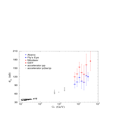
Figure 1: Total cross sections on $pp$ and $\bar{p}p$ from accelerator and cosmic-ray experiments (for complete list of references and tables see alm03 ).

Figure 2: Differential cross section data and the diffractive pattern from $pp$ elastic scattering at $\sqrt{s}=$ 52.8 GeV.

Figure 3: The slope parameter as function of the energy and determined in the interval 0.01 $<|t|<$ 0.20 GeV².

II.2 Principles, theorems and high-energy bounds

For our purposes, we recall some principles and theorems from axiomatic quantum field theories teo . The basic Principles are: Lorentz Invariance, Unitarity (related with the conservation of probability), Analyticity (related to causality) and Crossing (connecting particle-particle and particle-antiparticle interactions). Analyticity and crossing allow the connections between real and imaginary parts of the scattering amplitude by means of dispersion relations.

Several rigorous theorems and bounds may be deduced from the basic Principles and axiomatic quantum field theory. Among them, the Froissart-Martin bound concerns the increase of the total cross section stating that

$$\sigma_{tot}\leq C\log^{2}\frac{s}{s_{0}}\qquad{\rm as}\qquad s\rightarrow\infty.$$ (5)

The Pomeranchuk Theorem treats the difference between cross sections for particle-particle ($ab$) and particle-antiparticle scattering ($a\bar{b}$). The original form was deduced when it was believed that the cross section decreased to a constant value, and in this case $\sigma_{tot}^{ab}=\sigma_{tot}^{a\overline{b}}$ as $s\rightarrow\infty$. After the discovery of the rising of the cross section, Grunberg and Truong obtained the generalized or revised form of the Pomeranchuk Theorem, stating that

$$\frac{\sigma_{tot}^{ab}-\sigma_{tot}^{a\bar{b}}}{\sigma_{tot}^{ab}+\sigma_{tot}^{a\bar{b}}}\rightarrow 0\quad{\rm or}\quad\frac{\sigma_{tot}^{ab}}{\sigma_{tot}^{a\overline{b}}}\rightarrow 1\quad{\rm as}\quad s\rightarrow\infty,$$

and this means that, if the Froissart-Martin bound is reached, then

$$\Delta\sigma\equiv\sigma_{tot}^{a\overline{b}}-\sigma_{tot}^{ab}\leq C\frac{\sigma_{tot}^{a\overline{b}}+\sigma_{tot}^{ab}}{\log s}\leq C\log s.$$ (6)

By expressing the cross sections in terms of crossing even ($+$) and odd ($-$) contributions,

$$\sigma_{\pm}(s)=\frac{\sigma_{tot}^{ab}\pm\sigma_{tot}^{a\bar{b}}}{2},$$

we have $|\Delta\sigma|=|\sigma_{tot}^{a\overline{b}}-\sigma_{tot}^{ab}|=2\sigma_{-}$ . Therefore, $\Delta\sigma\equiv\sigma_{tot}^{a\overline{b}}-\sigma_{tot}^{ab}\rightarrow 0$ if and only if $\sigma_{-}\rightarrow 0$. This possible odd contribution is named Odderon and the case of even dominance at asymptotic energies is associated with the Pomeron.

II.3 Basic pictures

Nearly all the phenomenological models, able to describe the experimental data on elastic hadron scattering, are based on the Optical/Geometrical Picture (s-channel) and/or the Exchange Picture (t-channel). The corresponding formulas may be obtained from the Partial Waves representation of the scattering amplitude,

$$F(k,\theta)=\frac{i}{2k}\sum_{l=0}^{\infty}(2l+1)\left[1-e^{2i\delta_{l}}\right]P_{l}(\cos\theta),$$

where $\delta_{l}$ is the phase shift. In what follows, we outline the main steps and formulas in both pictures.

II.3.1 Optical/Geometrical Picture

From the partial wave representation, one considers the high-energy limit and the semi-classical approximation, so that the discrete angular momentum $l$ may be replaced by the continuum impact parameter $b$,

$$l=kb-\frac{1}{2}.$$

In turn, the discrete phase shifts $\delta_{l}$ are replaced by the continuum eikonal function of $b$ and $s$, $\chi(s,b)$ and

$$\sum_{l=0}^{\infty}...\ \ \rightarrow\ \ \int_{0}^{\infty}db...$$

The scattering amplitude in this Eikonal Representation, with azimuthal symmetry assumed, reads

$$F(s,q)=ik\int_{0}^{\infty}bdbJ_{0}(qb)[1-e^{i\chi(s,b)}].$$ (7)

The quantity

$$1-e^{i\chi(s,b)}\equiv\Gamma(s,b)$$ (8)

is named Profile function. From Unitarity this function is related to the probability that an inelastic event takes place at $b$ and $s$, the Inelastic Overlap function:

$$G_{inel}(s,b)=|\Gamma(s,b)|^{2}-2Re\Gamma(s,b).$$ (9)

Since in the Eikonal representation

$$\ G_{inel}(s,b)=1-e^{-2Im\chi(s,b)},$$ (10)

for $Im\ \chi(s,b)\geq 0$ we have $G_{inel}(s,b)\leq 1$, which implies in an automatically unitarized representation.

II.3.2 Exchange Picture

In this picture, from the partial wave representation, one considers the analytic continuation of the amplitude to complex angular momentum. In the asymptotic limit ($s\rightarrow\infty$) and with symmetry connecting the crossed channels one arrives at the Watson-Sommerfeld-Gribov-Regge representation for the scattering amplitude, expressed as a sum over the poles of the amplitude (the Regge poles), as outlined in what follows.

As it is known at high energies the number of partial waves is large, and one way to circumvent that is to transform the sum of partial waves into a complex integral, and then use the residues theorem to obtain a new sum, but involving only the number of residues:

$$\sum_{l=0}^{\infty}...\rightarrow\oint_{C}g(l)dl\rightarrow\sum_{m=0}^{N}\left.Res\ g(l)\right|_{l=l_{m}}.$$

Detailed calculation allows one to obtain the following representation for the scattering amplitude,

$$F(k,\theta)=\sum_{i=1}^{N}\frac{\beta_{i}(k)P_{\alpha_{i}(k)}(-\cos\theta)}{\sin\pi\alpha_{i}(k)}+BI(k,\theta),$$

where $BI(k,\theta)$ is called the Background integral. By considering the high-energy limit (then $BI\rightarrow 0$) and crossing (exchange four-momenta $p\rightarrow\quad\Leftrightarrow\quad\leftarrow-\bar{p}$) we can replace the crossing channel variable ($\bar{\theta}\leftrightarrow s$)

$$\cos\bar{\theta}=1-\frac{2s}{4m^{2}-t}\quad\rightarrow\quad\propto-s\quad{\rm as}\quad s\rightarrow\infty,$$

also,

$$P_{l}(x)\rightarrow\left[\frac{2^{l}\Gamma(l+1/2)}{\sqrt{\pi}\Gamma(l+1)}\right]x^{l}\quad{\rm for}\quad x\rightarrow\pm\infty,$$

and grouping all the $s$-independent quantities in a function ${\cal K}(t)$ we have

$$P_{\alpha(t)}(-\cos\bar{\theta})={\cal K}(t)s^{\alpha(t)}\quad{\rm for}\quad s\rightarrow\infty.$$

Rearranging the terms we arrive at a descending asymptotic series in powers of $s$, with leading contribution:

$$F(s,t)=\gamma(t)\xi(t)s^{\alpha(t)},$$ (11)

where $\gamma(t)$ is the residue function, $\xi(t)$ the signature factor and $\alpha(t)=\alpha(0)+\alpha^{\prime}t$ the trajectory function. This last function connects the spin and masses through the Chew-Frautschi plot, as exemplified in Fig. 4. In this picture the interaction of the colliding particles is basically interpreted in terms of exchanges of Regge poles (also Regge cuts) and the Pomeron (an ad hoc trajectory with intercept nearly above 1). We note that, as constructed, the exchange picture is intended for asymptotic energies.

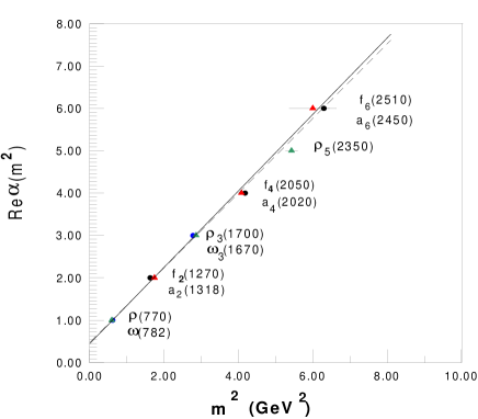
Figure 4: The Chew-Frautschi plot for some mesons and resonances.

III Analytic approach

The Analytic Approach for elastic hadron-hadron scattering is based on general principles and theorems from Quantum Field Theory. It is characterized by analytical parametrizations for the imaginary part of the forward amplitude, together with the use of dispersion relation techniques. The central point is the simultaneous investigation of the total cross section (imaginary part of the scattering amplitude, Eq. (2)) and the $\rho$ parameter (connected with the real part of the amplitude, Eq. (3)).

For particle-particle and particle-antiparticle interactions, dispersion relations are consequences of the principles of Analyticity and Crossing. In this context, they correlate real and imaginary parts of crossing even ($+$) and odd ($-$) amplitudes, which in turn are expressed in terms of the scattering amplitudes for a given process and its crossed channel, for example, $a+b$ and $a+\bar{b}$:

$$F_{ab}=F_{+}+F_{-},\qquad F_{a\bar{b}}=F_{+}-F_{-}.$$ (12)

At high energies, the standard singly subtracted integral dispersion relations, with poles removed, are given by

$$\mathop{\mathrm{Re}}F_{+}(s)=K+\frac{2s^{2}}{\pi}P\!\!\!\int_{s_{0}}^{+\infty}\!\!\!\ ds^{\prime}\frac{1}{s^{\prime}(s^{\prime 2}-s^{2})}\mathop{\mathrm{Im}}F_{+}(s^{\prime})$$ (13)

and

$$\mathop{\mathrm{Re}}F_{-}(s)=\frac{2s}{\pi}P\!\!\!\int_{s_{0}}^{+\infty}\!\!\!\ ds^{\prime}\frac{1}{(s^{\prime 2}-s^{2})}\mathop{\mathrm{Im}}F_{-}(s^{\prime}),$$ (14)

where $K$ is the subtraction constant and, for $pp$ and $\bar{p}p$ scattering, $s_{0}=2m^{2}\sim 1.8$ GeV².

In this section we review some results obtained through this approach. We start with the replacement of the above integral forms by derivative operators (Derivative Dispersion Relations) and then we discuss the use of analytic models (Reggeons, Pomeron, Odderon) for parametrizations involving the total cross section and the $\rho$ parameter, the determination of bounds for the soft Pomeron intercept, and the practical role of the subtraction constant.

In what follows we are mainly concerned with the $pp$ and $\bar{p}p$ elastic scattering, since for particle and antiparticle interactions they correspond to the highest energy interval with available data and are the only set including the cosmic-ray information on total cross sections ($pp$ scattering). As commented before, the experimental data available on the total cross sections (Figure 1) are characterized by discrepant experimental information at the highest energies, and one of our aims is to investigate the effects of these discrepancies in the context of the analytic models. This concern permeates all the discussion in this Section.

III.1 Derivative Dispertion Relations

The use of dispersion relations in the investigation of scattering amplitudes may be traced back to the end of fifties, when they were introduced in the form of Integral Dispersion Relations (IDR). Despite the important results that have been obtained since then, one limitation of the integral forms is their non-local character: in order to obtain the real part of the amplitude, the imaginary part must be known for all values of the energy. Moreover, the class of functions that allows analytical integration is limited.

In the last years, we have investigated the applicability of Derivative Dispersion Relations (DDR) in place of integral forms mmp ; alm01 ; almhadron02 ; alm03 ; lm03 ; am03 . In Reference am03 we present a recent review on different results and statements related to this replacement, and a discussion connecting these different aspects with the corresponding assumptions and classes of functions considered in each case.

In particular, we have shown that for the class of functions which are entire in the logarithm of the energy (as is the case of analytic models at high energies) it is possible to expand the integrand in the above formulas and by considering a high-energy approximation, represented by $s_{0}=2m^{2}\rightarrow 0$, to integrate term by term. In that case, as demonstrated in detail in am03 , the derivative dispersion relations with one subtraction reads

$$\frac{\mathop{\mathrm{Re}}F_{+}(s)}{s}=\frac{K}{s}+\tan\left[\frac{\pi}{2}\frac{\mathrm{d}}{\mathrm{d}\ln s}\right]\frac{\mathop{\mathrm{Im}}F_{+}(s)}{s},$$ (15)

$$\frac{\mathop{\mathrm{Re}}F_{-}(s)}{s}=\tan\left[\frac{\pi}{2}\left(1+\frac{\mathrm{d}}{\mathrm{d}\ln s}\right)\right]\frac{\mathop{\mathrm{Im}}F_{-}(s)}{s},$$ (16)

where the series expansion is implicit in the tangent operator. From this deduction one arrives to three formal results: (1) the subtraction constant is preserved when the IDR are replaced by DDR and, therefore, in principle, can not be disregarded in fit procedures; (2) except for the subtraction constant, the DDR with entire functions in the logarithm of the energy do not depend on any additional free parameter; (3) the only approximation involved in the replacement concerns the lower limit in the IDR (13-14), namely $s_{0}=2m^{2}\rightarrow 0$, which represents a high-energy approximation. In the next two subsections we discuss some uses of the DDR with analytical models, and in the third subsection we return to the replacement of IDR by DDR, investigating the important role of the subtraction constant from a practical point of view.

III.2 Basic Models

In this Subsection we make use of two basic and well known parametrizations for the total cross sections and investigate the effects of the discrepancies in the experimental information from cosmic-ray experiments.

III.2.1 Ensembles

In the cosmic-ray region, $6\ \textrm{TeV}<\sqrt{s}\leq 40$ TeV, the discrepancies on the total cross section information are due to both experimental and theoretical uncertainties in the determination of $\sigma_{tot}^{pp}$ from p-air cross sections. The situation has been recently reviewed in detail in alm03 , where a complete list of references, numerical tables and discussions are presented.

From Fig. 1 we see that, despite the large error bars in the cosmic-ray region, we can identify two distinct sets of estimations: one corresponding to the results by the Fly’s Eye Collaboration (Fly’s Eye) together with those by the Akeno Collaboration (Akeno); the other set associated with the results by Gaisser, Sukhatme, and Yodh (GSY) together with with those by Nikolaev (Nikolaev). Taken separately these two sets suggest different scenarios for the increase of the total cross section, as previously discussed in alm01 ; mm97 ; lm02 .

Based on these considerations, it is important to investigate the behavior of the total cross section by taking into account the discrepancies that characterize the cosmic ray information. To this end, in alm03 we have considered two ensembles of data and experimental information, as follows:

$\bullet$ Ensemble I: $\bar{p}p$ and $pp$ accelerator data + Akeno + Fly’s Eye;

$\bullet$ Ensemble II: $\bar{p}p$ and $pp$ accelerator data + Nikolaev + GSY.

To some extent, ensemble I represents a kind of high-energy standard picture and ensemble II a nonstandard one.

III.2.2 Analytic Models

With analytical parametrizations for $pp$/$\bar{p}p$ total cross sections, the connections with the $\rho$ parameter, Eq. (3), are obtained by defining the associated crossing even and odd quantities,

$$\sigma_{\pm}(s)=\frac{\sigma_{tot}^{pp}\pm\sigma_{tot}^{\bar{p}p}}{2},$$ (17)

using the high-energy normalization for the Optical Theorem,

$$\sigma_{tot}(s)\sim\frac{\mathop{\mathrm{Im}}F(s,0)}{s},$$ (18)

and the DDR given by Eqs. (15) and (16).

In alm03 we have considered two different parametrizations for the total cross sections, one introduced by Donnachie and Landshoff dl and other by Kang and Nicolescu kn . The main difference concerns the asymptotic limits, which allow the dominance of an even amplitude (Pomeron) or the odd amplitude (Odderon), respectively. In this way, we may contrast these possibilities with the standard and non-standard pictures represented by Ensembles I and II.

The Donnachie-Landshoff (DL) parametrization for the total cross sections is expressed by

$$\sigma_{tot}^{pp}(s)=Xs^{\epsilon}+Ys^{-\eta},\qquad\sigma_{tot}^{\bar{p}p}(s)=Xs^{\epsilon}+Zs^{-\eta},$$ (19)

where the first contribution is associated with a single Pomeron exchange (universal) and the second one with Reggeon exchange. With the procedure explained above, we obtain the analytical connections with the $\rho$ parameter for $pp$ and $\bar{p}p$ scattering:

$$\rho^{pp}(s)\sigma_{tot}^{pp}(s)=\frac{K}{s}+\left[X\tan\left(\frac{\pi\epsilon}{2}\right)\right]s^{\epsilon}$$

$$+ \left[\frac{(Y-Z)}{2}\cot\left(\frac{\pi\eta}{2}\right)-\frac{(Y+Z)}{2}\tan\left(\frac{\pi\eta}{2}\right)\right]s^{-\eta},$$

$$\rho^{\overline{p}p}(s)\sigma_{tot}^{\overline{p}p}(s)=\frac{K}{s}+\left[X\tan\left(\frac{\pi\epsilon}{2}\right)\right]s^{\epsilon}$$

$$+ \left[\frac{(Z-Y)}{2}\cot\left(\frac{\pi\eta}{2}\right)-\frac{(Y+Z)}{2}\tan\left(\frac{\pi\eta}{2}\right)\right]s^{-\eta}.$$

From the above formulas, since $\eta>0$, this model predicts that, asymptotically ($s\rightarrow\infty$),

$$\Delta\sigma =\ \sigma^{\overline{p}p}_{tot}(s)-\sigma^{pp}_{tot}(s)\rightarrow 0,$$

$$\Delta\rho =\ \rho^{\bar{p}p}(s)-\rho^{pp}(s)\rightarrow 0.$$

The parametrization for the total cross sections introduced by Kang and Nicolescu (KN), under the hypothesis of the Odderon, is given by

$$\sigma^{pp}_{tot}(s)=A_{1}+B_{1}\ln s+k\ln^{2}s,$$

$$\sigma^{\overline{p}p}_{tot}(s)=A_{2}+B_{2}\ln s+k\ln^{2}s+\frac{2R}{s^{1/2}},$$

and the connections with $\rho$ read

$$\rho^{pp}(s)\sigma_{tot}^{pp}(s)=\frac{K}{s}+\frac{\pi}{2}\left(\frac{B_{1}+B_{2}}{2}\right)$$

$$+ \left(\pi k+\frac{A_{2}-A_{1}}{\pi}\right)\ln s+\left(\frac{B_{2}-B_{1}}{2\pi}\right)\ln^{2}s-\frac{2R}{s^{1/2}},$$

$$\rho^{\overline{p}p}(s)\sigma_{tot}^{\overline{p}p}(s)=\frac{K}{s}+\frac{\pi}{2}\left(\frac{B_{1}+B_{2}}{2}\right)$$

$$+ \left(\pi k-\frac{A_{2}-A_{1}}{\pi}\right)\ln s-\left(\frac{B_{2}-B_{1}}{2\pi}\right)\ln^{2}s.$$

Differently from the previous case, this model predicts that the difference between the two cross sections is given by

$$\Delta\sigma =(A_{2}-A_{1})+(B_{2}-B_{1})\ln s+2Rs^{-1/2}$$

$$\rightarrow \Delta A+\Delta B\ln s\quad{\rm(asymptotically)},$$

so that, if $\Delta A\not=0$ and/or $\Delta B\not=0$, the total cross section difference may increase and $\sigma_{tot}^{pp}$ may even become greater than $\sigma_{tot}^{\bar{p}p}$, depending on the values and signs of $\Delta A$ and $\Delta B$, which is formally in agreement with the theorems of Sec. II.B. Moreover, if $\Delta A$ and $\Delta B$ are sufficiently small, so that we may replace $\sigma_{tot}^{\bar{p}p}\approx\sigma_{tot}^{pp}\equiv\sigma_{tot}(s)$, then, asymptotically,

$$\Delta\rho=\rho^{\overline{p}p}-\rho^{pp}\sim-\frac{1}{\pi\sigma_{tot}(s)}\left\{\Delta A\ln s+\Delta B\ln^{2}s\right\}.$$

This means that, depending on the fit results, there may be a change of sign in $\Delta\rho$, with $\rho^{pp}$ becoming greater than $\rho^{\overline{p}p}$ at some finite energy. Therefore, the case of a crossing either in $\sigma_{tot}$ or $\rho$ is a sign of the odderon contribution in the imaginary or real part of the amplitude, respectively.

III.2.3 Fits and Results

We have performed 16 different fits through the program CERN-MINUIT. In these fits we have used both ensembles I and II and both the DL and KN models. For each of these four possibilities we have performed global and individual fits to $\sigma_{tot}$ and $\rho$ and, in each case, we either considered the subtraction constant $K$ as a free fit parameter, or assumed $K=0$.

All the results are presented and discussed in detail in Ref. alm03 . Our main conclusions are the following: (1) Despite the small influence from different cosmic-ray estimations, the results allow to extract an upper bound for the soft Pomeron intercept: $1+\epsilon=1.094$; (2) although global fits present good statistical results, in general, this procedure constraints the rise of $\sigma_{tot}$; (3) the subtraction constant as a free parameter affects the fit results at both low and high energies; (4) independently of the cosmic-ray information used and the subtraction constant, global fits with the Odderon parametrization predict that, above $\sqrt{s}\approx 70$ GeV, $\rho_{pp}(s)$ becomes greater than $\rho_{\bar{p}p}(s)$, and this result is in complete agreement with all the data presently available. That result is displayed in Fig. 5 and we can infer $\rho_{pp}=0.134\ \pm\ 0.005$ at $\sqrt{s}=200$ GeV and $0.151\ \pm\ 0.007$ at $500$ GeV (BNL RHIC energies).

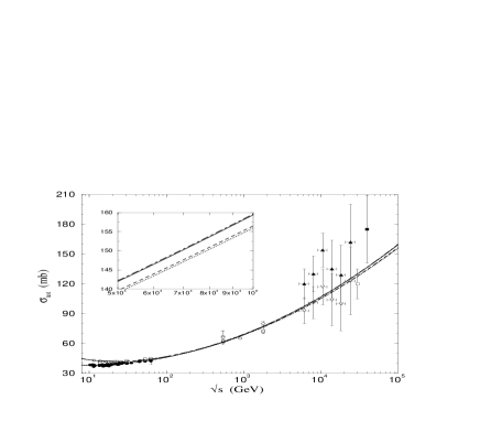
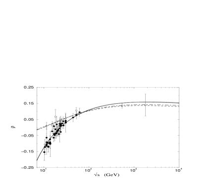
Figure 5: Simultaneous fits to $\sigma_{tot}(s)$ and $\rho(s)$ through the KN parametrization with $K=0$ and ensembles I (dotted curves for $pp$ and dashed for $\bar{p}p$) and II (solid curves for $pp$ and dot-dashed for $\bar{p}p$) alm03 .

III.3 Non-degenerate Meson Trajectories

The DL parametrization referred above assumes degeneracies between the secondary reggeons, imposing a common intercept for the $C=+1$ ($a_{2},f_{2}$) and the $C=-1$ ($\omega,\rho$) trajectories (see Fig. 4). More recently, analysis treating global fits to $\sigma_{tot}$ and $\rho$ have indicated that the best results are obtained with non-degenerate meson trajectories. In this case the forward scattering amplitude is decomposed into three reggeon exchanges, $F(s)=F_{\tt I\!P}(s)+F_{a_{2}/f_{2}}(s)+\tau F_{\omega/\rho}(s),$ where the first term represents the exchange of a single soft Pomeron, the other two the secondary Reggeons and $\tau=+1$ ($-1$) for $pp$ ($\bar{p}p$) amplitudes. Using the notation $\alpha_{\tt I\!P}(0)=1+\epsilon$, $\alpha_{+}(0)=1-\eta_{+}$ and $\alpha_{-}(0)=1-\eta_{-}$ for the intercepts of the Pomeron and the $C=+1$ and $C=-1$ trajectories, respectively, the total cross sections, Eq. (18), for $pp$ and $\bar{p}p$ interactions are written as

$$\sigma_{tot}(s)=Xs^{\epsilon}+Y_{+}\,s^{-\eta_{+}}+\tau Y_{-}\,s^{-\eta_{-}}$$ (20)

and the connection with the $\rho$ parameter by means of DDR is similar to that displayed in the last subsection.

Making use of this parametrization, in this section we present the determination of extrema bounds for the Pomeron intercept lm03 and a practical analysis on the replacement of IDR by DDR together with a discussion on the role of the subtraction constant am03 .

III.3.1 Extrema Bounds for the Pomeron Intercept

In order to analyze the extrema effects in the soft Pomeron intercept due to discrepancies in the experimental data, we performed a detailed analysis including the highest and the lowest values of the total cross section from both accelerators and cosmic-ray experiments.

As it is well known, in the accelerator region, the conflict concerns the results for $\sigma_{tot}^{\bar{p}p}$ at $\sqrt{s}=1.8$ TeV reported by the CDF Collaboration and those reported by the E710 and the E811 Collaborations (Fig. 1). In the cosmic-ray region, as we have discussed, the highest predictions for $\sigma_{tot}^{pp}$ concern the result by Gaisser, Sukhatme, and Yodh together with those by Nikolaev. In order to treat the lowest estimations in the cosmic-ray region, we consider the results obtained by Block, Halzen, and Stanev (BHS), by means of a QCD-inspired model. As discussed in alm03 , the reason for this choice is that, although the extracted $\sigma_{tot}^{pp}(s)$ shows agreement with the Akeno results, it is about $17$ mb below the Fly’s Eye value at $30$ TeV and therefore may be considered as a extreme lower estimate. All the numerical tables and references can be found in alm03 .

In this case we have considered the following ensembles of experimental information. First we only consider accelerator data in two ensembles with the following notation:

$\bullet$ Ensemble I: $\sigma^{pp}_{tot}$ and $\sigma^{\bar{p}p}_{tot}$ data ($10\leq\sqrt{s}\leq 900$ GeV) + CDF datum ($\sqrt{s}=1.8$ TeV);

$\bullet$ Ensemble II : $\sigma^{pp}_{tot}$ and $\sigma^{\bar{p}p}_{tot}$ data ($10\leq\sqrt{s}\leq 900$ GeV) + E710/E811 data ($\sqrt{s}=1.8$ TeV).

Ensemble I represents the faster increase scenario for the rise of $\sigma_{tot}$ from accelerator data and ensemble II the slowest one. These ensembles are then combined with the highest and lowest estimations for $\sigma_{tot}^{pp}$ from cosmic-ray experiments, namely, the Nikolaev and the Gaisser, Sukhatme, and Yodh (NGSY) results and the Block, Halzen, and Stanev (BHS) results, respectively. These new ensembles are denoted by

$\bullet$ I + NGSY

$\bullet$ II + BHS

As in the previous analysis, we have considered both individual fits to $\sigma_{tot}$, and simultaneous fits to $\sigma_{tot}$ and $\rho$, either in the case where the subtraction constant is considered as a free fit parameter or assuming $K=0$.

From this analysis, in the case of only accelerator data, we could infer the following upper and lower values for the Pomeron intercept: $\alpha_{\tt I\!P}(0)=1.098\pm 0.004$ (global fits to ensemble I, with $K=0$) and $\alpha_{\tt I\!P}(0)=1.085\pm 0.004$ (individual fit to $\sigma_{tot}$ from ensemble II), with bounds $1.102$ and $1.081$, respectively. Adding the cosmic-ray information, we inferred the following upper and lower values: $\alpha_{\tt I\!P}(0)=1.104\pm 0.005$ (individual fit to $\sigma_{tot}$ from ensemble I + NGSY) and $\alpha_{\tt I\!P}(0)=1.085\pm 0.003$ (global fits to ensemble II + BHS and $K$ as a free fit parameter or individual fit to $\sigma_{tot}$ from this ensemble), with bounds $1.109$ and $1.082$, respectively. Therefore we may infer the following extrema bounds for the soft Pomeron intercept:

$$\alpha^{upper}_{\tt I\!P}(0)=1.109,\qquad\alpha^{lower}_{\tt I\!P}(0)=1.081.$$

Figure 6 shows the total cross sections with parametrization (20) and the above extrema bounds, together with the experimental information available.

Figure 6: Fastest and slowest increase scenarios for the rise of the total cross section through parametrization (20) and allowed by the experimental information available: fits to ensembles I + NGSY (solid) and II (dashed) lmm03 .

Extensions of these extrema bounds for the pomeron intercept to meson-p, gamma-p and gamma-gamma scattering have been discussed in lmm03 . By means of global fits to total cross section data it is shown that these bounds are in agreement with the bulk of experimental data presently available, and extrapolations to higher energies indicate different behaviors for the rise of the total cross sections.

We have also obtained new constrained bounds for the Pomeron intercept from spectroscopy data (Chew-Frautschi plots) and have extended the analysis to baryon-p, meson-p, baryon-n, meson-n, gamma-p and gamma-gamma scattering lmm-npa04 . It is also presented tests on factorization and quark counting rules with both extrema and constrained bounds (asymptotic energy region). In particular, at 14 TeV (CERN LHC) the extrema and constrained bounds allow to infer $\sigma_{tot}=114\pm 25$ mb and $105\pm 10$ mb, respectively. lmm-npa04 .

III.3.2 IDR, DDR and the Subtraction Constant

As commented before, we have shown in Ref. am03 that for entire functions in the logarithm of the energy the only approximation involved in the replacement of IDR by DDR concerns the lower limit $s_{0}$ in the IDR: the high-energy condition is reached by assuming that $s_{0}=2m^{2}\rightarrow 0$ in Eqs. (13-14). In that paper we have investigated the practical applicability of the DDR and IDR in the context of the Pomeron-reggeon parametrizations, with both degenerate and non-degenerate higher meson trajectories. By means of global fits to $\sigma_{tot}(s)$ and $\rho(s)$ data from $pp$ and $\bar{p}p$ scattering, we have tested all the 16 important variants that could affect the fit results, namely the number of secondary reggeons, energy cutoff (5 and 10 GeV), effects of the high-energy approximation connected with the subtraction constant and the analytic approach using both DDR and IDR with fixed $s_{0}$. Our results led to the conclusion that the high-energy approximation and the subtraction constant affect the fit results at both low and high energies. This effect is a consequence of the fit procedure, associated with the strong correlation among the free parameters.

A striking novel result concerns the practical role of the subtraction constant. We have shown that, with the Pomeron-reggeon parametrizations, once the subtraction constant is used as a free fit parameter, the results obtained with the DDR and with the IDR (with finite lower limit, $s_{0}=2m^{2}$) are the same up to 3 significant figures in the fit parameters and $\chi^{2}/DOF$. This conclusion, as we have shown, is independent of the number of secondary reggeons (DL or extended parametrization) or the energy cutoff ($\sqrt{s}$ = 5 or 10 GeV). In Table I we display the fit results with the extended parametrization and cutoff at 10 GeV.

Table 1: Simultaneous fits to $\sigma_{tot}$ and $\rho$ through the extended parametrization, $\sqrt{s}_{\mathrm{min}}=$ 10 GeV (154 data points), with $K$ as a free parameter and using IDR with lower limit $s_{0}=2m^{2}$ and DDR am03 .

	IDR with $s_{0}=2m^{2}$	DDR
$X$	19.57 $\pm$ 0.79	19.58 $\pm$ 0.78
$Y_{+}$	66.0 $\pm$ 6.7	66.0 $\pm$ 6.6
$Y_{-}$	-29.2 $\pm$ 4.0	-29.2 $\pm$ 4.0
$\epsilon$	0.0897 $\pm$ 0.0033	0.0897 $\pm$ 0.0033
$\eta_{+}$	0.380 $\pm$ 0.033	0.380 $\pm$ 0.033
$\eta_{-}$	0.520 $\pm$ 0.025	0.520 $\pm$ 0.024
$K$	-14 $\pm$ 48	104 $\pm$ 58
$\chi^{2}/DOF$	1.10	1.10

IV Model Independent Analysis

This kind of analysis is characterized by model independent parametrizations of the experimental data involved and the extraction of empirical or semi-empirical information that can contribute with the development of phenomenological models and the underlying theory. In this section we review some results we have obtained in the investigation of $pp$ and $\bar{p}p$ differential cross section data (unconstrained and constrained fits, as will be explained) and the correlations between the experimental data on total cross section and the slope parameter (Eq. (4)).

IV.1 Differential Cross Section

Several authors have investigated elastic hadron scattering by means of parametrizations for the scattering amplitude and fits to the differential cross section data, Eq. (1). The extraction of the Profile, Eikonal and Inelastic Overlap functions in the $b$-space (impact parameter) and, in some special cases, the Eikonal in the $q^{2}$-space, has led to important and novel results related with geometrical aspects (radius, central opacity), differences between charge distributions and hadronic matter distributions, existence or not of eikonal zeros in the $q^{2}$-space and, more recently, connections with pomerons, reggeons and nonperturbative QCD aspects. In Ref. cmm03 we present a review and a critical discussion on the main results concerning this kind of analysis and also a wide list of references to outstanding works.

The basic input in all these analyses is the parametrization of the scattering amplitude as a sum of exponentials in $q^{2}$ (as empirically suggested by the diffractive pattern shown in Fig. 2) and fits to the differential cross section data. This parametrization allows analytical expressions for the Fourier transform of the amplitude, providing also analytical expressions for the quantities of interest in the $b$-space.

In the next two subsections we review the results we have obtained by means of unconstrained fits (fit parameters completely free, without extracted dependences on the energy) cmm03 ; cm , and discuss some research in course related to constrained fits (including dependences on the energy which are based on empirical information) acmmhadron04 .

IV.1.1 Unconstrained Fits and the Eikonal

In the high energy region, $\sqrt{s}>$10 GeV, differential cross section data are available at $\sqrt{s}=$ 13.8, 19.5, 23.5, 30.7, 44.7, 52.8 and 62.5 GeV for $pp$ scattering and at $\sqrt{s}=$ 13.8, 19.4, 31, 53, 62, 546 and 1800 GeV for $\bar{p}p$ scattering. Data from $pp$ scattering also exists at $\sqrt{s}=$ 27.5 GeV and 5.5 $\leq q^{2}\leq$ 14.2 GeV² (but not on $\sigma_{tot}$ and $\rho$), and as we shall show, that set plays a fundamental role in our analyse. See cmm03 for a complete list of references.

As discussed in cmm03 two main problems are typical of model independent analysis of the differential cross sections:

(1) Experimental data are available only over finite regions of the momentum transfer (which in general are small, $q^{2}<$ 7 GeV²) and the Fourier transform demands integration from $q^{2}$ = 0 to infinity. This means that any fit is biased by extrapolations and although some extrapolated curves may look unphysical, they can not be excluded on mathematical grounds.

(2) The exponential parametrization allows analytical determination of the quantities in the $b$-space (profile, inelastic, eikonal functions) and also the statistical uncertainties, by means of error propagation from the fit parameters. However, in this case, the translation of the eikonal from b-space to the $q^{2}$-space can not be analytically performed and neither the error propagation (through standard procedures). As a consequence, the unavoidable uncertainties from the fit extrapolations can not, in principle, be taken into account.

In what follows we review a model independent approach able to minimize the above two problems.

-

Fit Procedure

In order to treat problem (1) we have used the following procedure cm . Since it is known that for large $t$ the experimental data do not depend on the energy at $13.8$ GeV $\leq\sqrt{s}\leq 62$ GeV and that there exist data at $\sqrt{s}=27.5$ GeV in the region $5.5$ GeV${}^{2}\leq q^{2}\leq 14.2$ GeV², we have selected two ensembles of $pp$ and $\bar{p}p$ differential cross section data:

$\bullet$ Ensemble I: experimental data at each energy;

$\bullet$ Ensemble II: Ensemble I + data at $\sqrt{s}=27.5$ GeV.

For the scattering amplitude we have introduced the following model independent analytical parametrization for both real and imaginary parts:

$$F(s,q)=\{\mu\sum_{j=1}^{2}\alpha_{j}e^{-\beta_{j}q^{2}}\}+i\{\sum_{j=1}^{n}\alpha_{j}e^{-\beta_{j}q^{2}}\},$$ (21)

$$\mu=\frac{\rho(s)}{\alpha_{1}+\alpha_{2}}\sum_{j=1}^{n}\alpha_{j}.$$ (22)

With the experimental $\rho$ value at each energy the fits to the differential cross section data have been performed through the CERN-MINUIT routine and the validity or not of ensemble II is checked by means of the MINUIT output and standard statistical interpretation of the fit results (DOF, confidence levels).

For $pp$ scattering we have found that the data at $\sqrt{s}=$ 13.8 GeV are not compatible with ensemble II. In the case of $\bar{p}p$ scattering none of the data sets are compatible with ensemble II. Therefore, in what follows, ensemble II (data at $\sqrt{s}=$ 27.5 GeV added) corresponds only to $pp$ scattering at 6 energies: 19.5, 23.5, 30.7, 44.7, 52.8 and 62.5 GeV.

From the error matrix (variances and covariances), $\chi^{2}/DOF$ and confidence intervals, we infer the best values for the parameters and corresponding errors $\Delta\alpha_{j}$, $\Delta\beta_{j}$. By means of standard error propagation, the uncertainties in the free parameters, $\Delta\alpha_{j}$, $\Delta\beta_{j}$, ($j$ = 1, 2, …) have been propagated to the scattering amplitude, and then to the differential cross section, providing

$$\frac{d\sigma}{dq^{2}}\pm\Delta\left(\frac{d\sigma}{dq^{2}}\right).$$ (23)

By adding and subtracting the corresponding uncertainties we may estimate the confidence region associated with all the extrapolations, which cannot be excluded on statistical grounds. A typical result with ensembles I and II is illustrated in Fig. 7, for $pp$ scattering at $\sqrt{s}$= 23.5 GeV. We see that, as expected, the effect of adding the experimental data at $\sqrt{s}$= 27.5 GeV (when statistically justified) is to reduce drastically the uncertainty region. That result will be fundamental in the extraction of the empirical information on the eikonal, as shown in what follows.

Figure 7: Regions of uncertainties (limited by the solid lines) in fits to $pp$ differential cross section data, Eq. (23), at $\sqrt{s}=23.5$ GeV with ensembles I (below) and II (above) cmm03 .

-

Eikonal in the momentum transfer space

By means of the Fourier transform, Eqs.(7-8), the parametrization (21-22) provides analytical expressions for the real and imaginary parts of the Profile function, $\Gamma_{R}(s,b)$ and $\Gamma_{I}(s,b)$, and also the associated uncertainties. From the fit results, together with error propagation, we have found that

$$\frac{\Gamma_{I}^{2}(s,b)}{[1-\Gamma_{R}(s,b)]^{2}}\ll 1,$$

and therefore, the imaginary part of the eikonal may be approximated by

$$\chi_{I}(s,b)\approx\ln{1\over 1-\Gamma_{R}(s,b)}$$ (24)

and the uncertainty $\Delta\chi_{I}$ determined directly from $\Delta\Gamma_{R}$ through propagation.

The next step is to go to the momentum transfer space and concerns problem (2): the Fourier transform can not be performed analytically and therefore also the error propagation. For this reason we used a semi-analytical method as follows. Expanding the above equation, we express the remainder of the series as

$$R(s,b)=\ln[{1\over 1-\Gamma_{R}(s,b)}]-\Gamma_{R}(s,b)$$ (25)

and then fit the numerical points (MINUIT) by a sum of Gaussians in the impact parameter space:

$$R_{\rm{fit}}(s,b)=\sum_{j=1}^{6}A_{j}e^{-B_{j}b^{2}}.$$ (26)

A typical result is displayed in Fig. 8.

Figure 8: Typical parametrization for the generated remainder $R(s,b)$ by means of Eq. (26) cmm03 .

With this, the errors $\Delta A_{j}$ and $\Delta B_{j}$ may be propagated determining $\Delta R_{fit}(s,q)$ and then $\chi_{I}(s,q)\pm\Delta\chi_{I}(s,q)$. In order to check the results and approximations, we performed also numerical integration through the NAG routine.

- Results

One of the main results extracted from this analysis is the statistical evidence of eikonal zeros in the momentum transfer space, first presented in cm . In order to investigate the position of the zeros and, mainly, to determine the uncertainties in its values, we consider the expected behavior of $\chi_{I}$ at large $q^{2}$, namely $\chi_{I}\sim q^{-8}$. In Fig. (9) we show a typical plot of the quantity $q^{8}\chi_{I}(s,q)$ as function of $q^{2}$. The shaded areas correspond to the uncertainties obtained from error propagation. This example shows clearly the role and the effect of data at large values of the momentum transfer. In fact, within the uncertainties, ensemble I does not allow to infer a zero, but with ensemble II, we find statistical evidence for the change of sign.

Figure 9: The eikonal in the transfer momentum space (multiplied by $t^{4}$) for $pp$ at $\sqrt{s}=30.7$ GeV with ensemble I (above) and II (below) cmm03 .

From plots like that we can determine the positions of the zeros and the associated errors from the extrems of the uncertainty region (in general not symmetrical). The position of the zero can also be obtained from the numerical method, but without uncertainties.

In Figure 10 it is shown the position of the zeros as function of the energy determined by means of both the semi-analytical (with uncertainties) and numerical (without uncertainties) methods. Despite the systematic difference on the values with these methods, we may conclude that the position of the zero decreases as the energy increases. Roughly, $q^{2}_{0}:\ 8.5\rightarrow 6.0$ GeV² as $\sqrt{s}:\ 20\rightarrow 60$ GeV.

Figure 10: Position of the eikonal zero in the momentum transfer space as function of the energy cmm03 .

- Discussion

As reviewed in cmm03 , there has been previous indication of eikonal zeros in the momentum transfer space, but without associated uncertainties. Our first statistical evidence, published in 1997, indicated the position of the zero at $q^{2}_{0}=7\pm 2$ GeV² cm . In 2000, experiments performed at the Jefferson Laboratory, on electron-proton scattering, have indicated an unexpected decrease of the ratio between the electric and magnetic proton form factors as the momentum transfer increases from 0.5 to 5.6 GeV². Moreover, extrapolations from empirical fits indicate a change of sign (zero) in this ratio, just at $q^{2}\approx$ 7.7 GeV². Since for $pp$/$\bar{p}p$ scattering the eikonal is connected with the hadronic matter form factor (see Sec. V, Eq. (38)), the above results on the position of the zeros suggest novel and important insights on possible correlations between hadronic and electromagnetic interactions. We discuss that subject in mmmhadron04 , calling attention to the possibility of hadronic form factors depending on the energy.

We have also obtained the value of the imaginary part of the Eikonal at zero momentum transfer, that is, the central opacity. The results are displayed in Fig. 11. As discussed in cmmm , one naive way to test these results is with the Glauber model for the scattering involving hadrons $A$ and $B$, and the Optical Theorem at the elementary level. In that case, the elementary cross section may be expressed by

$$\sigma_{elem}(s)=\frac{4\pi}{N_{A}N_{B}}\chi_{I}(s,q=0),$$

where $N_{A}$ and $N_{B}$ are the number of constituents in hadrons $A$ and $B$, respectively. If we take $N_{A}=N_{B}=3$ we obtain $\sigma_{elem}\sim 6$ mb at the ISR region, a result in agreement with other estimations.

Figure 11: Imaginary part of the eikonal at zero momentum transfer, as function of the energy, from analysis on $pp$ and $\bar{p}p$ scattering cmm03 .

In Ref. cmm03 we discuss the applicability of our results in the phenomenological context, outlining some connections with nonperturbative QCD and presenting a critical review on the main results concerning “model-independent” analyses.

IV.1.2 Constrained Fits and Energy Dependence

Despite the results obtained with the parametrization discussed in the last subsection, due to the fit procedure, we do not have the dependence on the energy of the free parameters $\alpha_{i}$, $\beta_{i}$. Presently, we are investigating that subject and we review here some preliminary results acmmhadron04 .

The energy dependence has been introduced according to some empirical information: the increase of the total cross section and of the slope parameter with $\ln^{2}s$ and $\ln s$, respectively (see Figs 1 and 3). Let us consider the standard exponential parametrization for the imaginary part of the amplitude, normalized as

$$\frac{\mathop{\mathrm{Im}}F(s,q^{2})}{s}={\sum_{i=1}^{n}}{\alpha}_{i}\exp[-\beta_{i}q^{2}].$$ (27)

At $q^{2}=0$, from the optical theorem, Eq. (18), we expect a dependence of the parameters $\alpha_{i}$ with $\ln^{2}s$, and the slope represented by the parameters $\beta_{i}$ with $\ln s$. These are the central choices in our approach. In order to treat $pp$ and $\bar{p}p$ scatterings, in agreement with Analyticity and Crossing, we introduce crossing even and odd amplitudes and make use of the derivative dispersion relations, Eqs. (15) and (16), to connect real and imaginary parts of the amplitudes involved.

Specifically, for the imaginary part of the scattering amplitude we consider the parametrizations

$$\frac{\mathop{\mathrm{Im}}F_{pp}(s,q^{2})}{s}={\sum_{i=1}^{n}}{\alpha}_{i}(s)\exp[-\beta_{i}(s)q^{2}],$$ (28)

$$\frac{\mathop{\mathrm{Im}}F_{\bar{p}p}(s,q^{2})}{s}={\sum_{i=1}^{n}}{\bar{\alpha}}_{i}(s)\exp[-\bar{\beta}_{i}(s)q^{2}],$$ (29)

and, based on the above arguments, we introduce the following general dependences on the energy

$$\left\{\begin{array}[]{l@{\quad\quad}}\alpha_{i}(s)=A_{i}+B_{i}\ln(s)+C_{i}\ln^{2}(s)\\ \beta_{i}(s)=D_{i}+E_{i}\ln(s)\end{array}\right.$$ (32)

for $pp$ scattering and

$$\left\{\begin{array}[]{l@{\quad\quad}}\bar{\alpha}_{i}(s)=\bar{A}_{i}+\bar{B}_{i}\ln(s)+\bar{C}_{i}\ln^{2}(s)\\ \bar{\beta}_{i}(s)=\bar{D}_{i}+\bar{E}_{i}\ln(s)\end{array}\right.$$ (35)

for $\bar{p}p$ scattering, where $i=1,2,...n$. Defining the crossing even (+) and odd (-) amplitudes,

$$\mathop{\mathrm{Im}}F_{+}(s,q^{2})=\frac{\mathop{\mathrm{Im}}F_{pp}(s,q^{2})+\mathop{\mathrm{Im}}F_{\bar{p}p}(s,q^{2})}{2},$$ (36)

$$\mathop{\mathrm{Im}}F_{-}(s,q^{2})=\frac{\mathop{\mathrm{Im}}F_{pp}(s,q^{2})-\mathop{\mathrm{Im}}F_{\bar{p}p}(s,q^{2})}{2}.$$ (37)

the corresponding real parts can be determined by means of the leading terms of the DDR, Eqs. (15-16), and so the corresponding real parts of the $pp$ and $\bar{p}p$ amplitudes. With these analytic amplitudes we obtain the differential cross section:

$$\frac{d{\sigma}}{dq^{2}}=\frac{1}{16\pi s^{2}}|\mathop{\mathrm{Re}}F(s,q^{2})+i\mathop{\mathrm{Im}}F(s,q^{2})|^{2}.$$ (38)

In order to treat simultaneous fits to $pp$ and $\bar{p}p$ data we have considered only sets available at nearly the same energy, namely $\sqrt{s}\sim$ 19.5, 31, 53 and 62 GeV. As a preliminary test we make use of data at the diffraction peak, outside the Coulomb-nuclear interference region, 0.01 GeV${}^{2}<q^{2}\leq$ 0.5 GeV², and the data providing the optical point,

$$\frac{d\sigma(s,q^{2}=0)}{dq^{2}}=\frac{\sigma_{tot}(1+\rho^{2})}{16\pi}.$$ (39)

We have performed simultaneous fits to the experimental data through the MINUIT program. For this ensemble we used only two exponentials for the imaginary part of the amplitude, obtaining good reproduction of all the data analyzed, as shown in Fig. 12. In Ref. acmmhadron04 we also display the predictions for the differential cross sections at the RHIC energies. We are presently investigating the extension of the analysis to the region of higher momentum transfer.

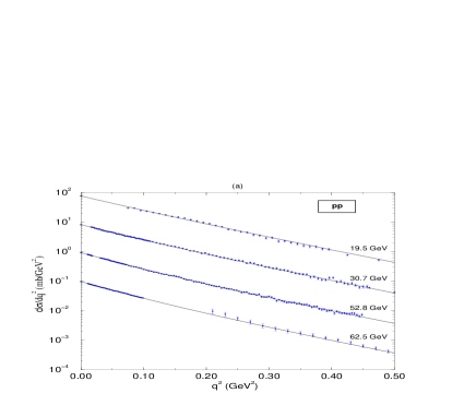
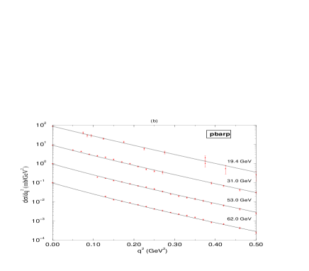
Figure 12: Differential cross section at the diffraction peak: fit results and experimental data (displaced by a factor of 10) acmmhadron04 .

IV.2 Total Cross Sections and Slopes

Another important quantity that characterizes the elastic hadron-hadron scattering is the slope parameter, defined in Eq. (4). In practice it may be determined by means of fits to the hadronic differential cross section data in the region of small momentum transfer, with the parametrization

$$\frac{d\sigma}{dt}=\left[\frac{d\sigma}{dt}\right]_{t=0}e^{-B|t|},$$ (40)

and, in general, it is connected with $\rho$ and $\sigma_{tot}$ through fits in the region of Coulomb interference bc . The slope and the total cross section are also important quantities in the determination of $\sigma_{tot}^{pp}$ from $\sigma^{p-air}$ (cosmic-ray experiments) but, as commented before, the procedure is strongly model dependent. One reason is associated with the use of the Glauber multiple diffraction formalism, in which $\sigma_{tot}(s)$ and $B(s)$ take part in the parametrization of the elastic amplitude,

$$F^{pp}(s,t)\propto\sigma_{tot}^{pp}(s)\exp\left\{\frac{B(s)t}{2}\right\}.$$ (41)

As commented in alm03 and mmmbjp04 , different models predict different relations between $\sigma_{tot}(s)$ and $B(s)$ and that is mirrored in the final value of the cross section, contributing to the discrepancies already discussed.

Based on the above observations, we have investigated the possibility to extract an empirical correlation between the experimental data on $\sigma_{tot}(s)$ and $B(s)$, from $pp$ and $\bar{p}p$ scatterings.

For the slope parameter, we have selected the data above the region of Coulomb-nuclear interference and below the “break” in the hadronic slope at the diffraction peak (localized at $|t|\sim$ 0.2 GeV² at the ISR and Collider energies), namely 0.01 $<|t|<$ 0.20 GeV² (Fig. (3)). In this region, the differential cross section data are well fitted by a single exponential and therefore there is no change in the slope associated with the $t$-dependence. For each energy we have compiled the corresponding data on the total cross section.

Once more, the choice for a parametrization was based on the empirical observation that at high energies $B(s)$ increases with the logarithm of $s$. Since the Kang-Nicolescu parametrization for the total cross section is expressed in terms of $\ln s$ (Sec. III.B.2), we replaced this dependence by the slope parameter:

$$\sigma_{tot}^{pp}(s) = c_{1}+c_{2}B+c_{3}B^{2},$$

$$\sigma_{tot}^{\overline{p}p}(s) = c_{1}+c_{2}B+c_{3}B^{2}+c_{4}e^{-B/2},$$ (42)

where $c_{i}$, $i=1,2,3,4$ are free fit parameters. That is a strictly mathematical choice, having nothing to do with the physics or model concept behind the Kang-Nicolescu parametrization.

Fits to the experimental data have been performed with the CERN-MINUIT program and the results are displayed in Fig. 13. It is expected that extrapolations to cosmic-ray energies may be useful in the determination of the $pp$ total cross section from $p$-air cross section, allowing to connect $\sigma_{tot}-B$ in an almost model independent way. We are presently investigating this subject.

Figure 13: Total cross sections in terms of the slope, and the parametrization (38) mmmbjp04 .

In Ref. mmmbjp04 we also made use of the Donnachie-Landshoff parametrization, which predicts a faster increase of the total cross section as function of the slope parameter. Moreover, in mmmbjp04 we also present a critical discussion on the recent measurement of the slope parameter at the BNL RHIC, at 200 GeV, by the pp2pp Collaboration. We call attention to the fact that the combination $B=$ 16.3 $\pm$ 1.8 GeV^-2 and $\sigma_{tot}=$ 51.6 mb, indicated by the pp2pp analysis, is in disagreement with the general trend for the behaviors of $\sigma_{tot}$ and $B$. If this “peer” is correct, new physics is necessary. Using the above $B$ value as input in our parametrizations, the corresponding values of the total cross sections show agreement with the $\sigma_{tot}$ versus $B$ data. However, these inferred values for $\sigma_{tot}$ indicate new physics when plotted as function of the energy. We conclude that if this measurement is correct and represents an hadronic quantity, its high value may indicate a “break” in the slope near 0.02 GeV², a phenomenon that was never observed in both $pp$ and $\bar{p}p$ scattering, at $\sqrt{s}\leq$ 62.5 GeV and $\sqrt{s}\leq$ 1.8 TeV, respectively and therefore, once more, new physics is necessary.

V Eikonal Models

It is expected that the eikonal function in the momentum transfer space, $\chi(s,q)$, may be connected with some microscopic aspects of the underlying field theory (elementary interactions, form factors, structure functions) and, as mentioned before, it corresponds to a unitarized scheme connected with the experimental data. Eikonal models are characterized by different choices for $\chi(s,q)$. In what follows we discuss our results and researches through two eikonal models (geometrical and QCD-based)

V.1 Geometrical Model - Inelastic Channel

In this subsection we review the description of $\bar{p}p$ multiplicities distributions (inelastic channel) from models for the elastic channel in the context of the geometrical picture (contact interactions).

- Elastic and Inelastic Channels

Through the Unitarity and the Inelastic Overlap Function, defined in Sec. II.C, we can connect elastic and inelastic scattering. This is done by expressing the topological cross section for producting an even number $n$ of charged particles at $s$ in terms of $G_{in}$:

$$\sigma_{n}(s)=\int d^{2}{\bf b}\ \sigma_{n}(s,b)=\int d^{2}{\bf b}\ G_{in}(s,b)\left[\frac{\sigma_{n}(s,b)}{G_{in}(s,b)}\right].$$

If $n(s)$ and $<n>_{(s)}$ are the hadronic and averaged multiplicities, respectively, by introducting the KNO variable $Z=n(s)/<n>_{(s)}$, the hadronic multiplicity distribution may be expressed by

$$\Phi(s,Z)=<n>_{(s)}\frac{\sigma_{n}(s)}{\sigma_{in}(s)}=\frac{\int d^{2}{\bf b}\frac{G_{in}(b,s)}{r(b,s)}\varphi(\frac{Z}{r(b,s)})}{\int d^{2}{\bf b}\ G_{in}(b,s)},$$

where $\varphi$ is the elementary multiplicity distribution and $r(b,s)=<n>_{(b,s)}/<n>_{(s)}$ the elementary multiplicity function.

In Ref. bmv , in the context of the geometrical picture, the elementary contact interaction process was based on $e^{+}e^{-}$ scattering data. In this approach we express

$$r(s,b)=\xi(s)\chi_{I}^{\gamma}(s,b),$$

where

$$\xi(s)=\frac{\int d^{2}b\ G_{in}(s,b)}{\int d^{2}b\ G_{in}(s,b)\chi_{I}^{\gamma}(s,b)}$$

and the power $\gamma$ is determined by fitting the average multiplicity from $e^{+}e^{-}$ scattering data through a power law parametrization:

$$<n>_{e^{+}e^{-}}=A[\sqrt{s}]^{\gamma}.$$

The elementary distribution $\varphi(Z/r(b,s))$ is represented by a Gamma distribution and determined also by fits to $e^{+}e^{-}$ data.

With inputs for $G_{in}(s,b)$ and/or $\chi_{I}(s,b)$, obtained from fits to elastic scattering data, we have no free parameter and the hadronic multiplicity distribution as function of $Z$ and $s$ may be inferred.

- Elastic-channel inputs and results

In Ref. bmv we made use of three inputs from the elastic sector. Two are based on the Multiple Diffraction Formalism, in which the eikonal in the momentum transfer space is expressed by

$$\chi(b,s)=C\int qdqJ_{0}(qb)G_{A}G_{B}f,$$ (43)

where $G_{A}$ and $G_{B}$ are the hadronic form factors, $f$ the elementary (constituent - constituent) amplitude and $C$ does not depend on the transferred momentum. In this case we made use of the parametrizations used by Chou and Yang and also by Menon and Pimentel. Both present good descriptions of the experimental data in the elastic channel. The other input corresponds to the Short Range Expansion of the inelastic overlap function, introduced by Henzi and Valin,

$$G_{in}(b,s)=P(s)\exp\{-b^{2}/4B(s)\}k(x,s),$$

with $k$ being expanded in terms of a short-range variable $x=b\ \exp\{-(\epsilon b)^{2}/4B(s)\}$, i.e.

$$k(x,s)=\sum_{n=0}^{N}\delta_{2n}(s)\left[\frac{\epsilon\ \exp\{1/2\}}{\sqrt{2B(s)}}\ x\right]^{2n}.$$

With particular parametrizations excellent agreement with experimental data on $pp$ and $\overline{p}p$ elastic scattering is achieved, allowing to infer the black-edge-large (BEL) behavior.

In Ref. bmv a detailed discussion is presented on several variants from the elastic channel and parametrizations from $e^{-}e^{+}$ scattering. In particular, the results for the multiplicities distributions, with the BEL inelastic overlap function, at $\sqrt{s}=$ 52.6 and 546 GeV are displayed in Fig. 14, together with the experimental data. The prediction shows that the violation of the KNO scaling is well described.

Figure 14: Scaled multiplicity distribution for inelastic $pp$ data at $\sqrt{s}=$ 52.6 GeV and $\bar{p}p$ data at 546 GeV, compared with the model predictions bmv .

V.2 QCD-inspired models

In this section we outline some research in course with the eikonal approach in connection with some QCD concepts. As we shall discuss the main point concerns the gluon-gluon contributions to the hadronic cross sections which we have investigated either from a dynamical gluon mass approach or by introducting the momentum scale in the gluonic distribution functions. After a review on the basic formalism we outline some aspects of both approaches.

V.2.1 Basic formalism

The formalism was introduced by Afek, Leroy, Margolis and Valin qcdb1 and developed by several authors, including (for our purposes) Durand, Pi dp , Block, Gregores, Halzen and Pancheri qcdb2 .

Originally, the point was to separate contributions from soft (S) and semi-hard (SH) inelastic processes by expressing

$$G_{inel}(s,b) = 1-\bar{P}_{S}\bar{P}_{SH}$$

$$= 1-e^{-2Re\ \chi_{S}(s,b)}e^{-2Re\ \chi_{SH}(s,b)},$$

where $\bar{P}_{S}$ is the probability of $NO$ soft inelastic process and $\bar{P}_{SH}$ the probability of $NO$ semi-hard inelastic process. Therefore, that indicated an additive contribution in the eikonal: $\chi(s,b)=\chi_{S}(s,b)+\chi_{SH}(s,b)$.

In the recent version by Block et al. qcdb2 different elementary contributions from quarks and gluons have been introduced: the gluon-gluon contribution comes from the parton model, the quark-quark from regge parametrization and the quark-gluon by phenomenological inputs. In what follows we shortly review the main formulas.

The normalization for the eikonal reads

$$F(s,q)=ik\int_{0}^{\infty}bdbJ_{0}(qb)\left[1-e^{i\chi(s,b)}\right],$$

$$\chi(s,b)=\mathop{\mathrm{Re}}\chi(s,b)+i\mathop{\mathrm{Im}}\chi(s,b).$$

For $pp$ and $\bar{p}p$ scattering the crossing even and odd contributions are expressed by $\chi_{p\bar{p}}=\chi^{+}+\chi^{-}$ and $\chi_{pp}=\chi^{+}-\chi^{-}$. The odd eikonal is assumed not to contribute at the asymptotic energies and is parametrized by

$$\chi^{-}(s,b)=C^{-}\frac{m_{0}}{\sqrt{s}}e^{i\pi/4}w(b,\mu_{odd}).$$

Analyticity (generation of real and imaginary parts) for the even part is assumed as given by the prescription

$$\chi^{+}(s,b)\quad \Rightarrow \quad\chi^{+}(se^{-i\pi/2},b)=$$

$$= Re\ \chi^{+}(s,b)+iIm\ \chi^{+}(s,b).$$

The even eikonal is expressed as a sum of three contributions, from quark-quark ($qq$), quark-gluon ($qg$) and gluon-gluon ($gg$) interactions,

$$\chi^{+}(s,b)=\chi_{qq}(s,b)+\chi_{qg}(s,b)+\chi_{gg}(s,b),$$

which individually factorize in $s$ and $b$,

$$\chi_{ij}(s,b)=i\sigma_{ij}(s)w(b,\mu_{ij}),$$

where $i,j=q,g$.

The impact parameter distribution function for each process comes from convolution involving dipole form factors (Chou-Yang Model):

$$w_{ii}(b,\mu_{ii})=\int d^{2}\vec{b}^{\prime}\rho_{i}(|\vec{b}^{\prime}|\rho_{i}(|\vec{b}-\vec{b}^{\prime}|),$$

$$\rho(b)=<G(q)>=<\frac{1}{(1+q^{2}/\mu^{2})^{2}}>,$$

where the angular brackets denote the symmetrical two-dimensional Fourier transform. Therefore,

$$w_{ii}(b)=\frac{1}{8}\frac{\mu_{ii}^{2}}{12\pi}[\mu_{ii}b]^{3}K_{3}(\mu_{ii}b),$$

and for $i\not=j$ it is assumed that

$$\mu_{ij}=\sqrt{\mu_{ii}\mu_{jj}}.$$

The elementary cross sections for each process are introduced as follows. The quark-quark contribution is parametrized as a constant plus a Regge (even) term,

$$\sigma_{qq}(s)=C+C_{R}^{+}\frac{m_{0}}{\sqrt{s}}$$

and the quark-gluon term as

$$\sigma_{qg}(s)=C_{qg}\log\frac{s}{s_{0}}.$$

The gluon-gluon contribution is considered as the responsible for the increase of the total cross section at the highest energies and is calculated through the parton model approach,

$$\sigma_{gg}(s)=c_{gg}\int_{0}^{1}d\tau F_{gg}(\tau)\hat{\sigma}_{gg}(\hat{s}),$$ (44)

with

$$F_{gg}=\int_{0}^{1}\int_{0}^{1}dx_{1}dx_{2}f_{g}(x_{1})f_{g}(x_{2})\delta(\tau-x_{1}x_{2}),$$ (45)

where $f_{g}(x_{i})$ is the gluon distribution function, $\tau=\hat{s}/s$, and the symbol $\hat{}$ denotes the elementary process. In qcdb2 the elementary cross section is given by

$$\hat{\sigma}_{gg}(\hat{s})=\frac{9\pi\alpha_{s}^{2}}{m_{0}^{2}}\theta(\hat{s}-m_{0}^{2}),$$ (46)

implying a cutoff $m_{0}$ for the particle production threshold and it is assumed the following simple parametrization for the gluon distribution function

$$f_{g}(x) = N_{g}\frac{(1-x)^{5}}{x^{1+\epsilon}},$$

$$N_{g} = \frac{1}{2}\frac{(6-\epsilon)(5-\epsilon)...(1-\epsilon)}{5!}.$$ (47)

The model has 6 fixed parameters, $m_{0}$, $\epsilon$, $\mu_{qq}$, $\mu_{gg}$, $\mu_{odd}$, $\alpha_{s}$ and 6 free parameters, determined from fits to $pp$ and $p\bar{p}$ forward scattering data, namely $\sigma_{tot}(s)$, $\rho(s)$ and $B(s)$ above 15 GeV qcdb2 . We have shown that the model applies only to forward and small momentum transfer regions lmmhadron02 .

In the next two sections we shall discuss two researches in course concerning the determination of the contribution from gluon-gluon interactions, Eqs. (39-42).

V.2.2 Dynamical gluon mass

The possibility that the gluon propagator may be regularized by a dynamically generated gluon mass cornwall has recently provided important phenomenological description of several processes natale . The approach allows to calculate the contribution for the elementary $gg$ cross section Eq. (42) and the main point is the association of the mass scale with the dynamical gluon mass. The basic ingredients are the expressions for the dynamical gluon mass,

$$M^{2}_{g}(\hat{s})=m_{g}^{2}\left[\frac{\ln[(\hat{s}+4{m_{g}}^{2})/\Lambda_{\mathrm{QCD}}^{2}]}{\ln[(4{m_{g}}^{2})/\Lambda_{\mathrm{QCD}}^{2}]}\right]^{-12/11},$$

and the associated running coupling constant

$$\alpha_{s}(\hat{s})=\frac{4\pi}{\beta_{0}\ln\left[(\hat{s}+4M_{g}^{2}(\hat{s}))/\Lambda_{\mathrm{QCD}}^{2}\right]},$$

where $\beta_{0}=11-\frac{2}{3}n_{f}$ and $n_{f}$ is the number of flavors. Preliminary tests with these contributions, in the context of the model described in the last subsection, have shown that the experimental data on $\sigma_{tot}(s)$, $\rho(s)$ and $B(s)$ are well described lmmmn , as exemplified in Fig. (15). We are presently investigating the contributions from the other elementary processes, $qq$ and $qg$.

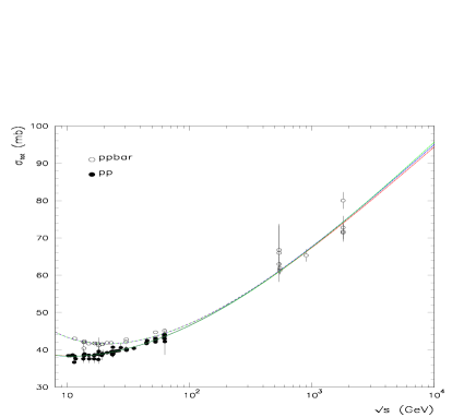
Figure 15: Description of the total cross sections through the QCD-based model with dynamical gluon mass $m_{0}=$ 500, 600 and 700 MeV lmmmn .

V.2.3 Momentum Scale

Presently, we are attempting to improve the descriptions of the QCD-inspired models by taking into account the momentum transfer scale in the gluon distribution functions. The point is to replace the simple choice in Eq. (42), by distribution functions with the $Q^{2}$ dependence, namely

$$f_{g}(x_{i})\rightarrow f_{g}(x_{i},Q^{2}).$$

That can be implemented, following the approach by Durand and Pi dp , by introducing the differential cross section

$$\hat{\sigma}_{gg}(\hat{s})=\int d|\hat{t}|\frac{d\hat{\sigma}_{gg}}{d|\hat{t}|}(\hat{s},\hat{t}),$$

with

$$\frac{d\hat{\sigma}_{gg}}{d|\hat{t}|}(\hat{s},\hat{t}) = \frac{9\pi\alpha_{s}^{2}}{2}[\frac{3}{\hat{s}^{2}}+\frac{\hat{t}}{\hat{s}^{3}}+\frac{\hat{t}^{2}}{\hat{s}^{4}}+\frac{1}{\hat{t}^{2}}+\frac{1}{\hat{s}\hat{t}}$$

$$- \frac{\hat{t}}{\hat{s}(\hat{s}+\hat{t})^{2}}]$$

and by considering $Q^{2}=|\hat{t}|$.

The novel input concerns the updated determinations of the gluon distribution functions (CETEQ6), parametrized by means of Chebyshev polynomials. Presently, the implementation in the QCD-inspired approach is being developed.

VI Nonperturbative QCD

As commented before the difficulties associated with high-energy soft processes arise from the fact that perturbative QCD can not be applied and presently we do not know how to calculate even the elastic hadron-hadron scattering amplitudes from a pure nonperturbative QCD formalism. However, progresses have been achieved through the approach introduced by Landshoff and Nachtmann landotto , developed by Nachtmann otto1 and connected with the Stochastic Vacuum Model (SVM) (introductory reviews may be found in rev ). In particular, through this formalism and in some restricted kinematic conditions, it is possible to connect the gluon two-point correlation function with elementary (quark-quark) scattering amplitude.

In this section we review the results we have obtained for these amplitudes with correlators determined from lattice QCD and also in the context of the Constrained Instantons.

VI.1 Stochastic Vacuum Model

The approach has its origins in the attempts by Landshoff and Nachtmann to connect soft high-energy processes with nonperturbative properties of the QCD vacuum, as for example, the gluon condensate introduced by Shifman, Vainstein and Zakharov svz . In the first version landotto quarks couple with Abelian gluons. The non-Abelian version was developed by Nachtmann in the context of QCD and using the eikonal method for high energy interactions otto1 . The scattering amplitude is calculated by means of a functional integral approach and is connected to a correlation function of two lightlike Wegner-Wilson loops. These correlation functions can be evaluated through the Stochastic Vacuum Model, in which the low frequency contributions to the functional integral of QCD are described in terms of a stochastic process by means of a cluster expansion svm . The model incorporates the gluon condensate concept and assumes that the correlation of two field strengths decreases rapidly with distance; due to an effective chromomagnetic monopole condensate, the QCD vacuum acts as a dual superconductor.

In this formalism the low frequencies contributions in the functional integral of QCD are described in terms of a stochastic process, by means of a cluster expansion. The most general form of the lowest cluster is the gauge invariant two-point field strength correlator svm ; dfk

$$< {\bf{F}}_{\mu\nu}^{\rm C}(x){\bf{F}}_{\rho\sigma}^{\rm D}(y)>=$$

$$= {\delta}^{\rm CD}g^{2}\frac{<FF>}{12(N_{c}^{2}-1)}\{({\delta}_{\mu\rho}{\delta}_{\nu\sigma}-{\delta}_{\mu\sigma}{\delta}_{\nu\rho}){\kappa}D({z^{2}/a}^{2})+$$

$$+ \frac{1}{2}[{\partial}_{\mu}(z_{\rho}{\delta}_{\nu\sigma}-z_{\sigma}{\delta}_{\nu\rho})+$$

$$+ {\partial}_{\nu}(z_{\sigma}{\delta}_{\mu\rho}-z_{\rho}{\delta}_{\mu\sigma})](1-{\kappa})D_{1}({z^{2}/a}^{2})\},$$

where $z=x-y$ is the two-point distance, $a$ is a characteristic correlation length, ${\kappa}$ a constant, $g^{2}<FF>$ the gluon condensate and $N_{c}$ the number of colours (${\rm C},{\rm D}=1,...,N_{c}^{2}-1$). The two scalar functions $D$ and $D_{1}$ describe the correlations and they play a central role in the application of the SVM to high energy scattering. Once one has information about $D$ and $D_{1}$, the SVM leads to the determination of the elementary quark-quark scattering amplitude, which constitutes important input for models aimed to construct hadronic amplitudes. The main formulas are as follows.

The elementary amplitude $f$ in the momentum transfer space is expressed in terms of the elementary profile $\gamma$ by

$$f(q^{2})=\int_{0}^{\infty}bdbJ_{0}(qb)\gamma(b).$$ (48)

In the Nachtmann approach the no-colour exchange parton-parton (loop-loop) amplitude can be written as

$$\gamma = {\langle}Tr[{\cal{P}}e^{-ig{\int}_{loop1}d{\sigma}_{\mu\nu}F_{\mu\nu}(x;w)}-1]$$

$$Tr[{\cal{P}}e^{-ig{\int}_{loop2}d{\sigma}_{\rho\sigma}F_{\rho\sigma}(y;w)}-1]{\rangle},$$

where ${\langle}{\rangle}$ means the functional integration over the gluon fields (the integrations are over the respective loop areas), and $w$ is a common reference point from which the integrations are performed. In the SVM by taking the Wilson loops on the light-cone the leading order contribution to the amplitude is given by

$$\gamma(b)=\eta{\epsilon}^{2}(b),$$ (49)

where $\eta$ is a constant depending on normalizations and

$$\epsilon(b)=g^{2}{\int}{\int}d{\sigma}_{\mu\nu}d{\sigma}_{\rho\sigma}Tr{\langle}F_{\mu\nu}(x;w)F_{\rho\sigma}(y;w){\rangle}.$$

After a two-dimensional integration, $\epsilon(b)$ can be expressed in terms of the correlation functions by

$$\epsilon(b)=\epsilon_{I}(b)+\epsilon_{II}(b),$$ (50)

where

$$\epsilon_{I}(b)={\kappa}{\langle}g^{2}FF{\rangle}{\int}_{b}^{\infty}db^{\prime}(b^{\prime}-b){\cal{F}}_{2}^{-1}[D(k^{2})](b^{\prime}),$$ (51)

$$\epsilon_{II}(b)=({1-\kappa}){\langle}g^{2}FF{\rangle}{\cal{F}}_{2}^{-1}[\frac{d}{dk^{2}}D_{1}(k^{2})](b).$$ (52)

For ${\cal{D}}=D$ or ${\cal{D}}=D_{1}$ we have ${\cal{D}}(k^{2})={\cal{F}}_{4}[{\cal{D}}(z^{2})]$, where ${\cal{F}}_{n}$ denotes a n-dimensional Fourier transform.

With the above formalism, once one has inputs for the correlation functions $D(z)$ and $D_{1}(z)$, the elementary amplitude in the momentum transfer space, Eq. (43), may, in principle, be evaluated through Eqs. (44-47). It is important to stress that, as constructed, the formalism is intended for small momentum transfer ($q^{2}\lesssim{\cal O}(1)$ GeV²) and asymptotic energies $s\rightarrow\infty$. Despite of these limitations, the investigation of soft high energy scattering at the energies presently available has led to satisfactory results dfk ; fp ; berger .

VI.2 Elementary Amplitudes

In this section we review the results we have obtained from inputs for the above correlators from lattice QCD mmt ; mm03 . We also comment the research in course in the semi-classical context of Instantons doro .

VI.2.1 Correlators from Lattice QCD

Numerical determinations of the above correlation functions, in limited interval of physical distances, exist from lattice QCD in both quenched approximation (absence of fermions) and full QCD (dynamical fermions included) digi .

With the procedure described above (see mmt for all the calculational details), the elementary scattering amplitude in the momentum transfer space can be determined in numerical form. In order to obtain analytical expressions, suitable for investigating distinct contributions and also for phenomenological uses, we have parametrized these numerical points through a sum of exponentials in $q^{2}$:

$$\frac{f(q^{2})}{f(0)}=\sum_{i=1}^{n}\alpha_{i}e^{-\beta_{i}q^{2}}.$$ (53)

The results are displayed in Fig. (16) from both quenched approximation and full QCD, together with the corresponding exponential components.

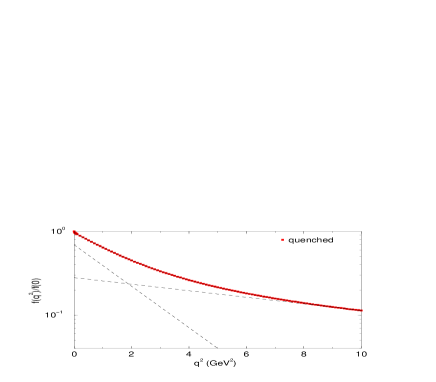
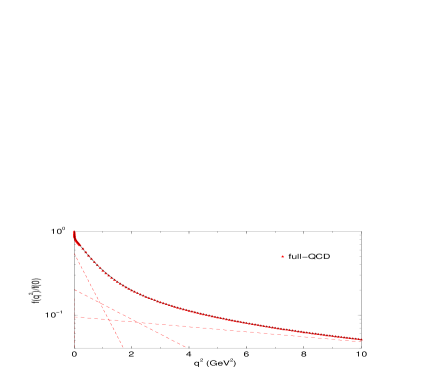
Figure 16: Elementary amplitudes from quenched and full QCD and the exponential components through parametrization (48) mm03 .

Our main conclusions are the following mm03 : (1) the amplitudes decrease smoothly as the momentum transfer increases and they do not present zeros; (2) the decreasing is faster when going from quenched approximation to full QCD (with decreasing quark masses), and this effect is associated with the increase of the correlation lengths; (3) the dynamical fermions generate two contributions in the region of small momentum transfer, which are of the same order at $q^{2}\sim$ 1 GeV² (only one contribution is present in the case of quenched approximation).

We understand that result (3) may suggest some kind of change in the dynamics at the elementary level, near $q^{2}\sim$ 1 GeV² and at asymptotic energies. If that is true, some signal could be expected at the hadronic level. One possibility is that this effect can be associated with the position of the dip (or the beginning of the “shoulder”) in the hadronic (elastic) differential cross section data. The asymptotic condition embodied in our result indicates that $q^{2}\sim$ 1 GeV² seems to be in agreement with the limit of the shrinkage of the diffraction peak, empirically verified when the energy increases in the region 23 GeV $\leq\sqrt{s}\leq$ 1.8 TeV.

VI.2.2 Correlators from the Instanton Approach

By means of the stochastic vacuum formalism we also presently investigate the elementary amplitudes using correlators determined in the context of the constraint instanton approach, developed by A. Dorokhov and collaborators instanton . The basic picture is that of an instanton field dominating at small distances and decreasing exponentially at large distances in the physical vacuum.

In Ref. doro , we make use of suitable parametrizations for the correlators and investigate the effects of the contributions from the short and long range correlations in the determination of the full correlator. Denoting those contributions as $D_{I}(z)$ and $D_{L}(z)$, respectively, we introduce a dimensionless parameter $\alpha\equiv\eta_{g}\rho_{c}$ in terms of the driven parameter $\eta_{g}$ and the size parameter $\rho_{c}$ doro . Since $\eta_{g}$ is correlated with the relative contribution of each kind of correlator, we consider two extreme cases: 1) equal contributions (weights 0.5 and 0.5), corresponding to $\alpha=1.0$; 2) almost pure instanton contribution (weights 0.99 and 0.01), corresponding to $\alpha=0.1$.

In the lack of information on the long range component, and for our purpose, we consider parametrization in a Gaussian form doro

$$D_{L}(z)=\exp\{-(2/2.5)^{2}z^{2}\}.$$

For the short range case, $\alpha=0.1$, we introduce the parametrization,

$$D_{I}(z) = 0.7119\exp\{-(2.403|z|)^{2}\}$$

$$+ 0.2899\exp\{-(1.485|z|)^{2}\}$$

$$- 9.456\times 10^{-3}\exp\{-1.277|z|\}.$$

The full correlator is then determined by

$$D(z)=0.99D_{I}(z)+0.01D_{L}(z).$$ (54)

For the long range case, $\alpha=1.0$, the parametrization takes the form

$$D_{I}(z) = 0.80084\exp\{-(2.3025|z|)^{2}\}$$

$$- 3.3846\times 10^{-2}\exp\{-(0.97119|z|)^{2}\}$$

$$+ 0.24225\exp\{-2.7706|z|\},$$

and for the full correlator we have

$$D(z)=0.5D_{I}(z)+0.5D_{L}(z).$$ (55)

With the Eqs. (49) and (50) we can calculate the elementary amplitude through the steps indicated in Sec. VI.A. The results are displayed in Fig. (17).

Figure 17: Elementary amplitudes from the constrained instanton approach.

A central result is that if the contribution from the long range correlator is small, that is, an almost purely instanton case, the corresponding elementary amplitude presents a minimum. In terms of the associated differential cross section, this implies a diffractive pattern in the momentum transfer space, a result already indicated in some phenomenological approaches menon ; mmt . In the case of equal weights the amplitude decreases monotonically with the momentum transfer.

We conclude that in the context of the instanton approach, the balance between the contributions of the short and long range correlators is a crucial point for the determination of the behavior of the elementary amplitudes. Further investigation along this line can bring new important insights on the connection between instanton correlators and the physical quantities which characterize the high-energy hadronic scattering.

VII Perspectives and Outlook

In this section we outline some perspectives in the area of high-energy elastic hadron scattering from both experimental and theoretical point of views. Certainly, some ideas may be biased by our own knowledge and our own personal view.

VII.1 Experiments

From the experimental point of view the perspectives are very optimistic due to the new generation of experiments with both accelerators and cosmic-ray observatories. Let us quickly summarize some projects in development.

The upgrade of the Fermilab Tevatron machine, together with upgrades and new devices in the CDF (Collider Detector Facility) and D0 detectors, are going to provide improved investigations on $\bar{p}p$ collisions at $\sqrt{s}\sim 2$ TeV. Although the main purpose of the experiment concerns hard diffraction, it will be possible to investigate elastic scattering in both high and low $q^{2}$ regions, the slope parameter, total cross section and single diffraction. Of topical importance for soft physics, the new determination of the total cross section shall possibly bring a solution for the puzzle represented by the discrepant results around $2$ TeV (E710/E811 and CDF).

At the Relativistic Heavy Ion Collider (RHIC) in the Brookhaven National Laboratory, $pp$ collisions are presently being investigated at energies never reached before: $\sqrt{s}:50\ -\ 500$ GeV. The experiment “Total and Differential Cross Sections and Polarization Effects in $pp$ Elastic Scattering at RHIC” (pp2pp) plans to investigate both elastic scattering and diffraction dissociation (single and double), in addition to spin effects. This will provide the first opportunity for direct comparison between $pp$ and $\bar{p}p$ scattering at the highest collider energies.

Although in a bit longer term, at the CERN Large Hadron Collider (LHC), the TOTEM experiment (Total Cross Section, Elastic Scattering and Diffraction Dissociation at the LHC) is specifically planned to study soft diffractive physics in $pp$ collisions at $\sqrt{s}\sim 16$ TeV. In particular, diffraction dissociation, total cross section and elastic scattering at large values of the momentum transfer will be investigated, up to $q^{2}=10\ -\ 15$ GeV². That will certainly allow discrimination and selection of various models and approaches, giving fundamental information at large momentum transfer; for example, showing the existence or not of structures. Moreover, this experiment will probably provide a final answer on the possible differences between $pp$ and $\bar{p}p$ total cross sections and the correct power $\gamma$ in the $\ln^{\gamma}s$ dependence of $\sigma_{tot}(s)$.

The most energetic event detected in cosmic-ray experiments had $E_{lab}=3\times 10^{20}$ eV, corresponding to an energy of $50$ Joules! Goals of the Auger project are the measurement of arrival direction and the energy and mass composition of cosmic rays above $E_{lab}=10^{19}$ eV. For $pp$ collisions this means $\sqrt{s}$ above $140$ TeV, nearly $10$ times the LHC energy. In addition to the astrophysical importance of the experiment, the measurement of the longitudinal development of showers will provide severe tests on hadronic interaction models. As a consequence, among others, the puzzles concerning the extraction of $pp$ cross section from $p-air$ production cross section may receive better insights, allowing more precise determinations and at energies possibly never to be reached by accelerator machines.

VII.2 Theory

Elastic hadron scattering (and soft diffractive processes in general) is a long distance phenomena and therefore we expect and look for a theoretical treatment via non-perturbative QCD. Despite all the difficulties mentioned along this manuscript, we understand that two approaches deserve special attention.

One of them concerns the approach by Nachtmann and the Stochastic Vacuum Model (Sec. VI.A) otto1 ; rev . Although under restrictive kinematic conditions (momentum transfer of the order or below 1 GeV², and asymptotic energies, $s\rightarrow\infty$) the formalism has provided interesting results in the investigation of the physical quantities that characterize the elastic $pp$ and $\bar{p}p$ scattering dfk ; berger , in special the works by Ferreira and Pereira, connecting experimental observables and QCD parameters fp . Attempts to implement the energy dependence in pure QCD grounds may be an important task for the near future.

The other approach is associated with evidences for finite gluon propagator and running coupling in the infrared region and that is the case in some classes of solutions of the nonperturbative Schwinger-Dyson equations. In particular, in the solution proposed by Cornwall cornwall the gluon acquires a dynamical mass leading to a freezing of the coupling constant in the infrared region. As referred before, Natale and collaborators natale have discussed several phenomenological tests, reaching interesting results which have permitted the development of the formalism and the selection of adequate basic inputs. That opens a new way to investigate long distance phenomena with a finite calculational approach.

We also understand that the connections between soft and semi-hard processes, typical of QCD-based models in the eikonal context, may bring new insights for the development of adequate calculational schemes in the nonperturbative treatment of high-energy elastic collisions.

VIII Summary and Final Remarks

Despite its simplicity, elastic hadron scattering constitutes a topical problem in high-energy Physics. Although the bulk of experimental data can be efficiently described in different phenomenological contexts, we are still facing the lack of a treatment and of a reasonable understanding of these processes based exclusively on QCD.

Our main strategy in investigating elastic scattering has been to look for descriptions based on the high-energy principles and theorems from Axiomatic Quantum Field Theory and, simultaneously, attempting to extract “empirical” information from all the experimental data available. Tests of discrepant data and their influence on the extracted information play a central role. In that way we hope to get feedbacks for theoretical development in nonperturbative and semi-hard QCD. We can summarize our main recent results as follows.

In the context of the Analytic Approach, we have investigated the effects of discrepant experimental information on the total cross sections in both accelerator and cosmic-ray energy regions. By means of analytical fits, we have obtained extrema bounds for the soft Pomeron intercept, namely $\alpha^{upper}_{\tt I\!P}(0)=1.109$ and $\alpha^{lower}_{\tt I\!P}(0)=1.081$. We have also obtained novel constrained bounds for the intercept from spectroscopy data (fitted Regge trajectories from Chew-Fautschi plots) and extended the analysis to several reactions. That information on the Pomeron bounds may be important for phenomenological developments and projects for new experiments. We have also shown that the presence of the Odderon in the real part of the elastic hadronic amplitude is not forbidden by the bulk of experimental data on $\sigma_{tot}$ and $\rho$. In particular, the fit with the Kang-Nicolescu parametrization has indicated a crossing in $\rho(s)$, with $\rho_{pp}$ becoming greater than $\rho_{\bar{p}p}$ above $\sqrt{s}$ = 70 GeV. That parametrization predicts $\rho_{pp}(\sqrt{s}=200\mathrm{GeV})=0.134\pm 0.005$ (RHIC regions). Detailed investigation on the applicability of DDR have shown that, once the subtraction constant is used as a free fit parameter, the DDR is equivalent to the IDR with finite lower limit ($s_{0}=2m^{2}$). That result was obtained for the class of entire functions in the logarithm of the energy (typical of analytic models).

In the context of Model Independent Analyses, we have investigated the correlations between the experimental data on total cross section and the slope parameter. The parametrization introduced is based on the empirical behavior of these quantities and extrapolations to cosmic-ray energies may be useful in the determination of proton-proton total cross sections from proton-air cross sections. By means of a novel model independent fit procedure to the differential cross section data, we have found statistical evidence for eikonal zero in the momentum transfer space and that the position of the zeros decreases as the energy increases. The zero position shows agreement with the result recently obtained for the electromagnetic form factor and inferred from elastic electromagnetic $e^{-}p$ scattering (polarization transfer experiments). Since our analysis concerns only hadronic interactions the results may bring new insights in the investigation of electromagnetic and hadronic form factors. We are also treating analytic fits with free parameters depending on the energy so as to develop a model independent predictive approach.

In the context of Eikonal Models we have obtained connections between the elastic and inelastic channel by means of the geometrical picture, and correlating $pp$ and $\bar{p}p$ scattering with contact interactions simulated by $e^{-}e^{+}$ distributions and multiplicities. With the class of QCD-based or QCD-inspired models we have developed novel gluonic contributions by means of two approaches. One is based in solutions of the Schwinger-Dyson equations characterized by the dynamical gluon mass. The other one is intended to take into account the $Q^{2}$- scale in updated gluonic distribution functions. Certainly, the two approaches are not independent, and we presently investigate their simultaneous implementation.

In the context of the Stochastic Vacuum Model, we have obtained novel results for the elementary scattering amplitudes, making use of correlators determined either from lattice QCD or from constrained instantons. In both cases the elementary amplitudes present no zeros (change of sign in the momentum transfer space). In the context of eikonal models, in which the eikonal is expressed in terms of the elementary amplitudes and form factors, Eq. (38), this result corroborates the interpretation of the zero in the hadronic form factor, and therefore, its dependence on the energy.

- (1) Y. Dokshitzer, Phil. Trans. Soc. London A395, 309 (2001).
- (2) M. M. Block and R. N. Cahn, Rev. Mod. Phys. 57, 563 (1985).
- (3) G. Matthiae, Rep. Prog. Phys. 57, 743 (1994).
- (4) E. Engel, Nucl. Phys. B (Proc. Suppl.) 82, 221 (2000).
- (5) E. Predazzi, in International Workshop on Hadron Physics 98, edited by E. Ferreira, F.F.S. Cruz and S.S. Avancini (World Scientific, Singapore, 1999) p. 80 - 175; V. Barone and E. Predazzi, High-Energy Particle Diffraction (Springer-Verlag, Berlim, 2002).
- (6) S. Donnachie, G. Dosch, P. Landshoff, O. Nachtmann, Pomeron Physics in QCD, Cambridge University Press, Cambridge, 2002.
- (7) M.J. Menon, “Introduction to Soft Diffraction: Some Results and Open Problems”, LISHEP 2002, Session B: Advanced School on High Energy Physics (2002).
- (8) A.F. Martini and E. Predazzi, Phys. Rev. D 66, 034029 (2002).
- (9) K. Hagiwara et al., Phys. Rev. D 66, 010001 (2002), Review of Particle Physics, Particle Data Group. Full data sets are available at http://pdg.lbl.gov.
- (10) R. F. Ávila, E. G. S. Luna, and M. J. Menon, Phys. Rev. D 67, 054020 (2003).
- (11) R.J. Eden, Rev. Mod. Phys. 43, 15 (1971); S.M. Roy, Phys. Rep. 5, 125 (1972); J. Fischer, Phys. Rep. 76, 157 (1981); P. Valin, Phys. Rep. 203, 233 (1991).
- (12) M. J. Menon, A. E. Motter, and B. M. Pimentel, Phys. Lett. B 451 , 207 (1999).
- (13) R. F. Ávila, E. G. S. Luna, and M. J. Menon, Braz. J. Phys. 31, 567 (2001).
- (14) R.F. Ávila, E.G.S. Luna, and M.J. Menon, in Proceedings of the VIII International Workshop on Hadron Physics 2002, edited by C.A.Z. Vasconcellos et al. (World Scientific, Singapore, 2003) p. 335.
- (15) E.G.S. Luna and M.J. Menon, Phys. Lett. B 565, 123 (2003).
- (16) R.F. Ávila and M.J. Menon, Nucl. Phys. A, 744, 249 (2004).
- (17) A.F. Martini, M.J. Menon, Phys. Rev. D 56, 4338 (1997).
- (18) E.G.S. Luna, M.J. Menon, in New States of Matter in Hadronic Interactions, PASI, AIP Conf. Proc. Vol. 631, edited by H.-Thomas Elze et al. (AIP. New York, 2002) pp. 721-722.
- (19) A. Donnachie and P.V. Landshoff, Z. Phys. C 2, 55 (1979); Phys. Lett. B 296, 227 (1992); Phys. Lett. B 387, 637 (1996).
- (20) K. Kang and B. Nicolescu, Phys. Rev. D 11, 2461 (1975); L. Lukaszuk and B. Nicolescu, Lett. Nuovo Cimento 8, 405 (1973).
- (21) E.G.S. Luna, M.J. Menon, J. Montanha, Braz. J. Phys. 34, 268 (2004).
- (22) E.G.S. Luna, M.J. Menon, J. Montanha, Nucl. Phys. A 745, 104 (2004).
- (23) P.A.S. Carvalho, A.F. Martini, M.J. Menon, Eur. Phys. J. C 39, 359 (2005).
- (24) P.A.S. Carvalho and M.J. Menon, Phys. Rev. D 56, 7321 (1997).
- (25) A.F. Martini, M.J. Menon, J. Montanha, “Zeros in the Electromagnetic and Hadronic Form Factors”, in IX Hadron Physics and VIII Relativistic Aspects of Nuclear Physics - A Joint Meeting on QCD and QGP, edited by M.E. Bracco, M. Chiapparini, E. Farreira, T. Kodama, AIP Conf. Proc. Vol. 739 (AIP, New York, 2004) pp. 578 - 580.
- (26) P.A.S. Carvalho, A.F. Martini, M.J. Menon, A.E. Motter, in International Workshop on Hadron Physics 98, Florianópolis, 1998, edited by E. Ferreira, F.F. de Souza Cruz and S.S. Avancini (World Scientific, Singapore, 1999) p. 326.
- (27) R.F. Ávila, S.D. Campos, M.J. Menon, and J. Montanha, “Analytical Fits to Hadron-Hadron Differential Cross Section Data at the Diffraction Peak”, in IX Hadron Physics and VIII Relativistic Aspects of Nuclear Physics - A Joint Meeting on QCD and QGP, edited by M.E. Bracco, M. Chiapparini, E. Farreira, T. Kodama, AIP Conf. Proc. Vol. 739 (AIP, New York, 2004) pp. 529 - 531.
- (28) A.F. Martini, M.J. Menon, J. Montanha, Braz. J. Phys. 34, 263 (2004).
- (29) P.C. Beggio, M.J. Menon, and P. Valin, Phys. Rev. D 61, 034015 (2000); in International Conference on Elastic and Diffractive Scattering - Blois VIII, edited by V.A. Petrov and A.V. Prokudin (World Scientific, Singapore, 2000) pp. 371 - 376.
- (30) Y. Afek, C. Leroy, B. Margolis, P. Valin, Phys. Rev. Lett. 45, 85 (1980).
- (31) L. Durand and H. Pi, Phys. Rev. Lett. 58, 303 (1987); Phys. Rev. D 38, 78 (1988); Phys. Rev. D 40, 1436 (1989).
- (32) M.M. Block, E.M. Gregores, F. Halzen, G. Pancheri, Phys. Rev. D 60, 054024 (1999).
- (33) E.G.S. Luna, A.F. Martini, and M.J. Menon, in Proceedings of the VIII International Workshop on Hadron Physics 2002, edited by C.A.Z. Vasconcellos et al. (World Scientific, Singapore, 2003) p. 295.
- (34) J. M. Cornwall, Phys. Rev. D26 (1982) 1453; J. M. Cornwall and J. Papavassiliou, Phys. Rev. D40 (1989) 3474, D44 (1991) 1285.
- (35) M. B. Gay Ducati, F. Halzen and A. A. Natale, Phys. Rev. D48, 2324 (1993); F. Halzen, G. Krein and A. A. Natale, Phys. Rev. D47, 295 (1993); A. C. Aguilar, A. Mihara and A. A. Natale, Phys. Rev. D65, 054011 (2002), Int. J. Mod. Phys. A19, 249 (2004); A. C. Aguilar, P. S. R. da Silva and A. A. Natale, Phys. Rev. Lett. 90, 152001 (2003);
- (36) E.G.S. Luna, A.F. Martini, M.J. Menon, A. Mihara, A.A. Natale, “Preliminary results on the influence of a gluon mass in hadronic scattering” in IX Hadron Physics and VIII Relativistic Aspects of Nuclear Physics - A Joint Meeting on QCD and QGP, edited by M.E. Bracco, M. Chiapparini, E. Farreira, T. Kodama, AIP Conf. Proc. Vol. 739 (AIP, New York, 2004) pp. 572 - 574.
- (37) P.V. Landshoff, O. Nachtmann, Z. Phys. C 35, 405 (1987).
- (38) O. Nachtmann, Ann. Phys. 209, 436 (1991).
- (39) O. Nachtmann, “High-Energy Collisions and Nonperturbative QCD”, hep-ph/96093; O. Nachtmann, in International Workshop on Hadron Physics 2000, edited by F.S. Navarra, M.R. Robilotta, G. Krein (World Scientific, 2001) p. 152-216; H.G. Dosch, in International Workshop on Hadron Physics 96, edited by E. Ferreira et al. (World Scientific, 1997) pp. 169-219.
- (40) M.A. Shifman, A.I. Vainshtein, V.I. Zakharov, Nucl. Phys. B 147, 385, 448, 519 (1979).
- (41) H.G. Dosch, Phys. Lett. B 190, 177 (1987); H.G. Dosch, Yu. A. Simonov, Phys. Lett. B 205, 339 (1988); Yu. A. Simonov, Nucl. Phys. B 307, 512 (1988); 204, 67 (1989); A. Krämer, H.G. Dosch, Phys. Lett. B 252, 669 (1990); 272, 114 (1991).
- (42) H.G. Dosch, E. Ferreira and A. Krämer, Phys. Rev. D 50, 1992 (1994); Phys. Lett. B 318, 197 (1993); 289, 153 (1992).
- (43) E. Ferreira and F. Pereira, Phys. Rev. D 55, 130 (1997); Phys. Rev. D 56, 179 (1997); Phys. Lett. B 399, 177 (1997); Phys. Rev. D 59, 014008 (1998); Phys. Rev. D 61, 077507 (2000); E. Ferreira, Braz. J. Phys. 30, 282 (2000).
- (44) E.R. Berger, O. Nachtmann, Eur. Phys. J. C 7, 459 (1999).
- (45) M.J. Menon, Nucl. Phys. B (Proc. Suppl.) 25, 94 (1992); Phys. Rev. D 48, 2007 (1993); Can. J. Phys. 74, 594 (1996).
- (46) A.F. Martini, M.J. Menon, D.S. Thober, Phys. Rev. D 57, 3026 (1998).
- (47) A.F. Martini and M.J. Menon, Phys. Lett. B 570, 53 (2003).
- (48) A. Dorokhov. A.F. Martini, M.J. Menon, in XX Brazilian National Meeting on Particles and Fields (1999), www.sbf1.if.usp.br/eventos/enfpc/xx/procs/res68/.
- (49) A. Di Giacomo and H. Panagopoulos, Phys. Lett. B 285 (1992) 133; A. Di Giacomo, E. Meggiolaro, and H. Panagopoulos, Nucl. Phys. B 483 (1997) 371; M. D’Elia, A. Di Giacomo, E. Meggiolaro, Phys. Lett. B 408 (1997) 315.
- (50) A.E. Dorokhov, S.V. Esaibegian, A.E. Maximov, S.V. Mikhailov, Eur. Phys. J. C 13, 331 (2000).