Subtraction at NNLO

Abstract:

We propose a framework for the implementation of a subtraction formalism at NNLO in QCD, based on an observable- and process-independent cancellation of infrared singularities. As a first simple application, we present the calculation of the contribution to the $e^{+}e^{-}$ dijet cross section proportional to $C_{\scriptscriptstyle F}T_{\scriptscriptstyle R}$.

1 Introduction

The hard dynamics of processes involving hadrons is nowadays remarkably well described by QCD predictions. An important role has been played in this achievement by the ability to compute the relevant reactions to next-to-leading order (NLO) accuracy, a mandatory step in view of the large value of the coupling constant $\alpha_{\scriptscriptstyle S}$. Although fairly successful in their phenomenological applications, NLO predictions are affected by uncertainties that can be of the order of a few tens of percent, typically estimated by varying the renormalization and factorization scales. This is a consequence of the fact that, in some cases, NLO corrections are numerically as important as the leading order (LO) contributions. By increasing the accuracy of the perturbative predictions, through the computation of the next-to-next-to-leading order (NNLO) contributions, one would certainly reduce the size of the uncertainties, and obtain a firmer estimate of the rates [1]. Such a task, however, implies finding the solution of a few highly non trivial technical problems. Recently, two major bottlenecks have been cleared: two-loop functions with up to four legs have been computed (with zero or one massive leg) [2], and so have the three-loop Altarelli-Parisi kernels [3], which opens the way to exact NNLO PDF fits.

The present situation is thus fairly similar to that of the early 80’s. Back then, the computation of the two-loop Altarelli-Parisi kernels [4], and the ability to compute all the tree-level and one-loop functions for specific processes, left open the problem of achieving explicitly the cancellation of soft and collinear singularities, as predicted by the Kinoshita-Lee-Nauenberg (KLN) theorem for inclusive, infrared-safe observables. Early approaches pioneered the subtraction [5] and phase-space slicing [6] techniques, for computing analytically the divergent part of the real corrections, in the context of the prediction for a given observable; a different observable required a novel computation. Later, it was realized that the KLN cancellation could be proven in an observable- and process-independent manner, which allows one to predict any observable (for which the relevant matrix elements can be computed) to NLO accuracy without actually using the observable definition in the intermediate steps of the computation [7]–[10]. Apart from being very flexible, these universal methods have the virtue of clarifying the fundamental structure of the soft and collinear regimes of QCD.

Observable- and process-specific calculations have certain advantages over universal formalisms; the possibility of exploiting the observable definition and the kinematics of a given reaction in the intermediate steps of the computation generally leads to more compact expressions to integrate. This is evident if we consider the fact that the first NNLO results for total rates [11, 12] pre-date the universal NLO formalisms by some years. More recently, the first calculation of a rapidity distribution at NNLO has been performed using these techniques, for single vector boson hadroproduction [13, 14].

In the last two years a fair amount of work has been carried out in the context of process-specific calculations. The structure of NNLO infrared-singular contributions necessary to implement the subtraction method has been discussed in the case of $e^{+}e^{-}\to 2~{}{\rm jets}$ [15], and the $C_{\scriptscriptstyle F}^{3}$ contribution to $e^{+}e^{-}\to 3~{}{\rm jets}$ has been computed [16]. Moreover, an observable-independent method [17], based on sector decomposition [18], has been recently proposed. This approach allows one to handle and cancel infrared singular contributions appearing in the intermediate steps of an NNLO calculation in a fully automatic (numerical) way, and thus significantly differs from the semi-analytical approaches of refs. [7]–[10]. This method has been applied to the computations of $e^{+}e^{-}\to 2~{}{\rm jets}$ [19] and Higgs hadroproduction [20] cross sections.

One may argue that, since the number of two-loop amplitudes computed so far is limited, process-specific (but observable-independent) computations such as those of refs. [16, 19, 20] are all what is needed for phenomenology for several years to come. Although this is a legitimate claim, we believe that universal formalisms are interesting in themselves, and that their achievement should be pursued in parallel to, and independently of, that of process-specific computations. Work in this direction is currently being performed by various groups, and partial results are becoming available [21]–[28]. We stress that the formulation of universal subtraction formalisms at NNLO would pave the way to the matching between fixed-order computations and parton-shower simulations, similarly to what recently done at NLO [29, 30], thus resulting in predictions with a much broader range of applicability for phenomenological studies.

The purpose of the present paper is to propose a general framework for the implementation of an observable- and process-independent subtraction method. A complete formalism would require the construction of all of the NNLO counterterms necessary to cancel soft and collinear singularities in the intermediate steps of the calculation, as well as their integration over the corresponding phase spaces. Most of the recent work on the subject concentrated on the former aspect, without performing the analytical integration of the kernels. In this paper we take a different attitude: we propose a subtraction formula, and we give a general prescription for the construction of all of the counterterms. However, we do not construct most of them explicitly here, since we limit ourselves to considering only those relevant to the $C_{\scriptscriptstyle F}T_{\scriptscriptstyle R}$ part of the dijet cross section in $e^{+}e^{-}$ collisions. On the other hand, we specifically address the problem of their integration. We propose general formulae for the phase spaces necessary for the integration of the subtraction kernels, and we use them to integrate the counterterms mentioned above. In this way, we directly prove that the subtraction formula we propose does allow us to cancel the singularities at least in the simple case of the $C_{\scriptscriptstyle F}T_{\scriptscriptstyle R}$ contribution to the $e^{+}e^{-}\to 2~{}{\rm jets}$ cross section, and we construct a numerical code with which we recover the known results for dijet and total rates. Since the subtraction formula, the counterterms, and the phase-space measures are introduced in a way which is fully independent of the hard process considered, this result gives us confidence that the framework we propose here is general enough to lead to the formulation of a complete subtraction formalism, whose explicit construction is, however, beyond the scope of the present paper.

The paper is organized as follows: in sect. 2 we review the strategy adopted by NLO universal subtraction formalisms, and we formulate it in language suited to its extension to NNLO. Such an extension is discussed in sect. 3, and our main NNLO subtraction formula is introduced there. This subtraction procedure is shown to work in a simple case in sect. 4. We present a short discussion in sect. 5, and give our conclusions in sect. 6. A few useful formulae are collected in appendices A and B.

2 Anatomy of subtraction at NLO

Let us denote by $r$ any real (tree-level) matrix element squared contributing to the NLO correction of a given process, possibly times a measurement function that defines an infrared-safe observable, and by $d\Phi$ the phase space. For example, when considering two-jet production in $e^{+}e^{-}$ collisions, $r$ is the product of the $\gamma^{*}\to q\bar{q}g$ matrix element squared times the $\delta$ functions that serve to define the jets within a given jet-finding algorithm, and $d\Phi$ is the three-body phase-space for the final-state partons $q$, $\bar{q}$, and $g$. As is well known, the integral

$$R=\int rd\Phi$$ (1)

is in general impossible to compute analytically. In the context of the subtraction method, one rewrites eq. (1) as follows:

$$R=\int\left(rd\Phi-\tilde{r}d\tilde{\Phi}\right)+\int\tilde{r}d\tilde{\Phi}\,.$$ (2)

The quantities $\tilde{r}$ and $d\tilde{\Phi}$ are completely arbitrary, except for the fact that $\tilde{r}d\tilde{\Phi}$ must fulfill two conditions: the first integral in eq. (2) must be finite, and the second integral must be calculable analytically; when this happens, $\tilde{r}d\tilde{\Phi}$ is called a subtraction counterterm. The former condition guarantees that the divergences of $\int\!\tilde{r}d\tilde{\Phi}$ are the same as those of $\int\!rd\Phi$. Thus, by computing $\int\!\tilde{r}d\tilde{\Phi}$ one is able to cancel explicitly, without any numerical inaccuracies, the divergences of the one-loop contribution, as stated by the KLN theorem; when using dimensional regularization with

$$d=4-2\epsilon$$ (3)

the divergences will appear as poles $1/\epsilon^{k}$, with $k=1,2$. As far as the first integral in eq. (2) is concerned, its computation is still unfeasible analytically. However, being finite, one is allowed to remove the regularization, by letting $\epsilon\to 0$, and to compute it numerically.

In the context of the subtraction method, the computation of an observable to NLO accuracy therefore amounts to finding suitable forms for $\tilde{r}$ and $d\tilde{\Phi}$, that fulfill the conditions given above. Clearly, it is the asymptotic behaviour of $r$ in the soft and collinear configurations that dictates the form of $\tilde{r}$. The major difficulty here is that soft and collinear singularities overlap, and $\tilde{r}$ should not oversubtract them. To show how to construct $\tilde{r}$ systematically, let us introduce a few notations. We call singular limits those configurations of four-momenta which may lead to divergences of the real matrix elements. Whether the matrix elements actually diverge in a given limit depends on the identities of the partons whose momenta are involved in the limit; for example, no singularities are generated when a quark is soft, or when a quark and an antiquark of different flavours are collinear. We call singular (partonic) configurations the singular limits associated with given sets of partons, and we denote them as follows:

• Soft: one of the partons has vanishing energy.

  $$S_{i}:\;\;\;\;\;\;p_{i}^{0}\to 0.$$ (4)

• Collinear: two partons have parallel three-momenta.

  $$C_{ij}:\;\;\;\;\;\;\vec{p}_{i}\parallel\vec{p}_{j}.$$ (5)

• Soft-collinear: two partons have parallel three-momenta, and one of them is also soft.

  $$SC_{ij}:\;\;\;\;\;\;(p_{i}^{0}\to 0,\vec{p}_{i}\parallel\vec{p}_{j}).$$ (6)

The singular limits will be denoted by $S$, $C$, and $SC$, i.e. by simply removing the parton labels in eqs. (4)–(6). In practice, in what follows parton labels will be often understood, and singular limits will collectively indicate the corresponding partonic configurations.

For any function $f$, which depends on a collection of four-momenta, we introduce the following operator:

$${\cal E}_{\scriptscriptstyle NLO}(f)=f-\sum_{i}f(S_{i})-\sum_{i<j}f(C_{ij})-\sum_{ij}f(SC_{ij}),$$ (7)

where $f(L_{\alpha})$, $L_{\alpha}=S_{\alpha},C_{\alpha},SC_{\alpha}$ is the asymptotic behaviour of $f$ in the singular partonic configuration $L_{\alpha}$. Notice that the role of indices $i$ and $j$ is symmetric in the collinear limit, but is not symmetric in the soft-collinear one (see eqs. (5) and (6)), and this is reflected in the sums appearing in the third and fourth terms on the r.h.s. of eq. (7). The asymptotic behaviour $f(L_{\alpha})$ is always defined up to non-singular terms; however, what follows is independent of the definition adopted for such terms. Although all of the singularities of $f$ are subtracted on the r.h.s. of eq. (7), ${\cal E}_{\scriptscriptstyle NLO}(f)$ is not finite, owing to the overlap of the divergences. To get rid of this overlap, we introduce a set of formal rules, that we call the ${\cal E}$-prescription:

1. Apply ${\cal E}_{\scriptscriptstyle NLO}$ to $f$, getting $f+\sum_{\alpha_{1}}f_{\alpha_{1}}^{(1)}$.

2. Apply ${\cal E}_{\scriptscriptstyle NLO}$ to every $f_{\alpha_{1}}^{(1)}$ obtained in this way and substitute the result in the previous expression, getting $f+\sum_{\alpha_{1}}f_{\alpha_{1}}^{(1)}+\sum_{\alpha_{2}}f_{\alpha_{2}}^{(2)}$.

3. Iterate the procedure until ${\cal E}_{\scriptscriptstyle NLO}(f_{\alpha_{n}}^{(n)})=f_{\alpha_{n}}^{(n)}$, $\forall\,\alpha_{n}$, at fixed $n$.

4. Define $\tilde{f}=-\sum_{i}\sum_{\alpha_{i}}f_{\alpha_{i}}^{(i)}$.

In order to show explicitly how the ${\cal E}$-prescription works, let us apply it step by step. After the first iteration, we find eq. (7). With the second iteration, we need to compute

$${\cal E}_{\scriptscriptstyle NLO}(f(S_{i})) = f(S_{i})-\sum_{j\neq i}f(S_{i}\oplus S_{j})-\sum_{j<k}f(S_{i}\oplus C_{jk})-\sum_{jk}^{j\neq i}f(S_{i}\oplus SC_{jk}),\phantom{aaa}$$ (8)

$${\cal E}_{\scriptscriptstyle NLO}(f(C_{ij})) = f(C_{ij})-\sum_{k}f(C_{ij}\oplus S_{k})-\sum_{k<l}^{\{i,j\}\neq\{k,l\}}f(C_{ij}\oplus C_{kl})$$ (9)

$$-\sum_{kl}^{\{i,j\}\neq\{k,l\}}f(C_{ij}\oplus SC_{kl}),$$

$${\cal E}_{\scriptscriptstyle NLO}(f(SC_{ij})) = f(SC_{ij})-\sum_{k}^{k\neq i}f(SC_{ij}\oplus S_{k})-\sum_{k<l}^{\{i,j\}\neq\{k,l\}}f(SC_{ij}\oplus C_{kl})$$ (10)

$$-\sum_{kl}^{\{i,j\}\neq\{k,l\}}f(SC_{ij}\oplus SC_{kl}),$$

where we denoted by $f(L_{\alpha_{1}}\oplus L_{\alpha_{2}})$ the asymptotic behaviour of the function $f(L_{\alpha_{1}})$ in the singular partonic configuration $L_{\alpha_{2}}$. Although in general the operation $\oplus$ is non commutative, we shall soon encounter examples in which $f(L_{\alpha_{1}}\oplus L_{\alpha_{2}})=f(L_{\alpha_{2}}\oplus L_{\alpha_{1}})$. Notice that we included all possible singular parton configurations in eqs. (8)–(10), except for the redundant ones – an example of which would be the case $k=i$ in the second term on the r.h.s. of eq. (10).

We now have to take into account the fact that we are performing a computation to NLO accuracy. Thus, the definition of an observable will eventually be encountered (for example, embedded in a measurement function), which will kill all matrix element singularities associated with a partonic configuration that cannot contribute to the observable definition at NLO. For example, the limit in which two partons are soft is relevant only to beyond-NLO results, and this allows us to set $f(S_{i}\oplus S_{j})=0$ $\forall\{i,j\}$; analogously

$$\sum_{k}f(C_{ij}\oplus S_{k})=f(C_{ij}\oplus S_{i})\,,$$ (11)

since the case $k\neq i$ would result into two unresolved partons, which is again a configuration that cannot contribute to NLO. In general, it is easy to realize that the operator ${\cal E}_{\scriptscriptstyle NLO}$ is equivalent to the identity when it acts on the terms generated in the second iteration of the ${\cal E}$-prescription (i.e., the terms with negative signs in eqs. (8)–(10)), and thus that, according to the condition in item 3 above, the ${\cal E}$-prescription requires at most two iterations at NLO (it should be stressed that this would not be true in the case of an infrared-unsafe observable, which would lead to an infinite number of iterations). It follows that

$$\tilde{f}=\sum_{i}f(S_{i})-\sum_{ij}f(S_{i}\oplus C_{ij})+\sum_{i<j}f(C_{ij})-\sum_{ij}f(C_{ij}\oplus S_{i})+\sum_{ij}f(SC_{ij}).$$ (12)

This expression can be further simplified by observing that the soft and the collinear limits commute. This allows one to write

$$f(S_{i}\oplus C_{ij})=f(C_{ij}\oplus S_{i})=f(SC_{ij}),$$ (13)

and therefore

$$\tilde{f}=\sum_{i}f(S_{i})+\sum_{i<j}f(C_{ij})-\sum_{ij}f(SC_{ij}).$$ (14)

Let us now identify $f$ with $rd\Phi$. Eq. (14) implies that the term added and subtracted in eq. (2) reads

$$\tilde{r}d\tilde{\Phi}=\sum_{i}r(S_{i})d\Phi(S_{i})+\sum_{i<j}r(C_{ij})d\Phi(C_{ij})-\sum_{ij}r(SC_{ij})d\Phi(SC_{ij}).$$ (15)

All that is needed for the construction of a subtraction counterterm at NLO is eq. (15), and the definition of the rules for the computations of $r(L)$ and $d\Phi(L)$. In other words, all subtraction procedures at NLO are implementation of eq. (15), i.e. of the ${\cal E}$-prescription, within a computation scheme for the asymptotic behaviours of the matrix elements and the phase spaces. Although not strictly necessary in principle, it is always convenient to adopt the same procedure for the computation of $r(L)$ and of $d\Phi(L)$; most conveniently, this is done by first choosing a parametrization for the phase space, and by eventually using it to obtain $r(L)$.

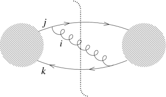
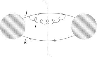
Figure 1: Configurations contributing to soft (left panel) and collinear (right panel) limits of squared amplitudes.

In order to be more specific, we shall consider two explicit constructions of subtraction counterterms, namely those of ref. [8] and of ref. [9]. Since the subtractions always need to be performed at the level of amplitudes squared, the relevant diagrams (in a physical gauge) are those depicted in fig. 1, for the soft (left panel) and collinear (right panel) limits respectively. According to the notations introduced before and the parton labelings that appear in the diagrams, we denote the corresponding singular partonic configurations by $S_{i}$ and $C_{ij}$. As is well known, the leading (singular) behaviours of the real matrix elements squared will be given by the following factors (see e.g. ref. [31])

$$S_{i}\;\longrightarrow\;\frac{p_{j}\!\cdot\!p_{k}}{p_{i}\!\cdot\!p_{j}p_{i}\!\cdot\!p_{k}}\,,$$ (16)

$$C_{ij}\;\longrightarrow\;\frac{1}{p_{i}\!\cdot\!p_{j}}\,,$$ (17)

with the parton $k$ playing no role in the collinear limit. In order to integrate the subtraction counterterms analytically, a phase space parametrization must be chosen such that the leading divergences displayed in eqs. (16) and (17) have as trivial as possible a dependence upon the integration variables. Furthermore, the eikonal and collinear factors of eqs. (16) and (17) have manifestly overlapping divergences; thus, a matching treatment of the two, while not strictly necessary, would allow an easy identification of the overlapping contributions.

In ref. [8] the phase space is first decomposed in a manner which is largely arbitrary, but such that in each of the resulting regions only one soft and one collinear singularity at most can arise (i.e., the other singularities are damped by the $\Theta$ functions which are used to achieve the partition); the two may also occur simultaneously. Thus, each region is identified by a pair of parton indices – say, $i$ and $j$ – and no singularity other than $1/p_{i}\!\cdot\!p_{j}$ can occur in that region. This implies that the eikonal factor in eq. (16) will not contribute a divergence to the region above when $\vec{p}_{i}\parallel\vec{p}_{k}$.

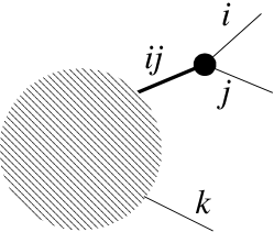
Figure 2: Splitting topology contributing to NLO computations.

In turn, this makes possible to choose a parametrization of the phase space, based on exact factorization formulae (see app. B), in which a pseudo-parton $i\!j$ (thick line in fig. 2) branches into on-shell partons $i$ and $j$ (narrow lines); in other words, the phase space of eq. (1) is written as follows:

$$d\Phi=d\Phi_{n-1}(i\!j)d\overline{\Phi}_{2}(i,j)\,,$$ (18)

where $d\overline{\Phi}$ is the two-body phase space, times the measure over the virtuality of the branching pseudo-parton $i\!j$. The parton $k$ may or may not serve to define the integration variables, but is irrelevant in the treatment of the singularities. Clearly, this parametrization is suggested by a collinear-like configuration, but thanks to the partition of the phase space it also allows a straightforward integration over soft singularities. Graphically, this is equivalent to squaring the parts of the diagrams in fig. 1 which lay to the left of the cut. The contribution due to the part to the right of the cut in the diagram on the left panel is clearly recovered once the sum over parton labels is carried out, since the role of indices $j$ and $k$ is fully symmetric. Once the exact parametrization of eq. (18) is fixed, ref. [8] proceeds by defining

$$d\Phi(L)=d\Phi_{n-1}(\widetilde{i\!j})d\overline{\Phi}_{2}(i,j;L)\,,$$ (19)

where $\widetilde{i\!j}$ is an on-shell parton, and

$$d\overline{\Phi}_{2}(i,j;S_{i}) = d\overline{\Phi}_{2}(i,j)\Big{|}_{p_{i}^{0}\to 0}\,,$$ (20)

$$d\overline{\Phi}_{2}(i,j;C_{ij}) = d\overline{\Phi}_{2}(i,j)\Big{|}_{\vec{p}_{i}\parallel\vec{p}_{j}}\,,$$ (21)

$$d\overline{\Phi}_{2}(i,j;SC_{ij}) = d\overline{\Phi}_{2}(i,j)\Big{|}_{p_{i}^{0}\to 0,\vec{p}_{i}\parallel\vec{p}_{j}}\,,$$ (22)

are obtained by neglecting constant terms in the corresponding limits. Obviously, $d\Phi(L)$ is not an exact representation of the full phase space any longer, i.e. $d\Phi(L)\neq d\Phi$; however, this does not introduce any approximation in the procedure, since the subtraction counterterm is subtracted and added back in the physical cross section (eq. (2)). Finally, the asymptotic behaviours $r(L)$ appearing in eq. (15) are directly taken from factorization formulae, eqs. (16) and (17), without any further manipulation.

In the dipole formalism of ref. [9], the following identity is exploited

$$\frac{1}{p_{i}\!\cdot\!p_{j}p_{i}\!\cdot\!p_{k}}=\frac{1}{p_{i}\!\cdot\!p_{j}p_{i}\!\cdot\!(p_{j}+p_{k})}+\frac{1}{p_{i}\!\cdot\!p_{k}p_{i}\!\cdot\!(p_{j}+p_{k})}$$ (23)

for the eikonal factor of eq. (16). The two terms on the r.h.s. of eq. (23) are symmetric for $j\leftrightarrow k$, and thus only the first one actually needs to be considered. As far as collinear configurations are concerned, this term is singular only when $\vec{p}_{i}\parallel\vec{p}_{j}$, but not when $\vec{p}_{i}\parallel\vec{p}_{k}$. Thus, the identity in eq. (23) has the same function as the partition of the phase space of ref. [8]. Furthermore, an exact parametrization of the phase space is chosen

$$d\Phi=d\Phi_{n-1}(\widetilde{i\!j};k)d\overline{\Phi}_{2}(i,j;k)$$ (24)

which differs from the one of eq. (18) in that the parton $k$ (called the spectator) plays a fundamental role, since it allows to put on shell the splitting pseudo-parton even if $i$ and $j$ are not exactly collinear, or $i$ is not soft. Thanks to this property, in ref. [9] we have

$$d\Phi(L)=d\Phi\,,\;\;\;\;\;\;\;\;L=S_{i},C_{ij},SC_{ij},$$ (25)

and thus eq. (15) becomes

$$\tilde{r}d\tilde{\Phi}=D_{ij;k}d\Phi\,,$$ (26)

$$D_{ij;k}=r(S_{i;k})+r(C_{ij})-r(SC_{ij})\,,$$ (27)

where $r(S_{i;k})$ is obtained by taking the soft limit of the real matrix element, and keeping only the first term on the r.h.s. of eq. (23).

In summary, the common feature of refs. [8, 9] is the fact that, by disentangling (with different techniques) the two collinear singularities that appear in each eikonal factor, they define subtraction formalisms based on building blocks which all have a collinear-like topology; we shall denote by ${\bf 1}$ this topology, depicted in fig. 2 (the parton labels are obviously irrelevant for topological considerations), a notation which is reminiscent of a branching after which the list of resolved partons is diminished by one unity. The explicit expressions for the building blocks, which originate from the soft, collinear, and soft-collinear limits and include the treatment of the phase space, depend on the formalism; however, in all cases they are combined according to eq. (15), i.e. according to the ${\cal E}$-prescription, in order to construct the sought subtraction counterterm.

3 Subtraction at NNLO

In this section, we shall introduce a general framework for the implementation of a subtraction method to NNLO accuracy. We shall consider the process

$$e^{+}e^{-}\,\longrightarrow\,n~{}{\rm jets}\,.$$ (28)

In this way, all the intricacies are avoided due to initial-state collinear singularities, which allows us to simplify the notation considerably. The systematic construction of the subtraction counterterms that we propose in the following will however be valid also in the case of processes with initial-state hadrons, since the procedure is performed at the level of short-distance partonic cross sections. On the other hand, we do not present here the explicit parametrizations of the phase spaces for the case of initial-state partons, and we do not consider the contributions of initial-state collinear counterterms which are necessary in order to achieve the complete cancellation of infrared singularities for processes with QCD partons in the initial state.

3.1 Generalities

At NNLO, the process (28) receives contribution from the following partonic subprocesses

$$e^{+}e^{-}\,\longrightarrow\,m~{}{\rm partons},\;\;\;\;\;\;m=n,\,n+1,\,n+2.$$ (29)

We write the amplitude corresponding to eq. (29) in the following way

$${\cal M}_{m}=g_{\scriptscriptstyle S}^{m-2}{\cal M}_{m}^{(0)}+g_{\scriptscriptstyle S}^{m}{\cal M}_{m}^{(1)}+g_{\scriptscriptstyle S}^{m+2}{\cal M}_{m}^{(2)}+\dots,$$ (30)

where ${\cal M}_{m}^{(0)}$, ${\cal M}_{m}^{(1)}$ and ${\cal M}_{m}^{(2)}$ are the tree-level, one-loop and two-loop contributions to the process (29) respectively. Squaring eq. (30) we get:

$$\left|{\cal M}_{n}\right|^{2} = g_{\scriptscriptstyle S}^{2n-4}\left|{\cal M}_{n}^{(0)}\right|^{2}+g_{\scriptscriptstyle S}^{2n-2}\left({\cal M}_{n}^{(0)}{\cal M}_{n}^{(1)^{\star}}+{\cal M}_{n}^{(0)^{\star}}{\cal M}_{n}^{(1)}\right)$$ (31)

$$+g_{\scriptscriptstyle S}^{2n}\left(\left|{\cal M}_{n}^{(1)}\right|^{2}+{\cal M}_{n}^{(0)}{\cal M}_{n}^{(2)^{\star}}+{\cal M}_{n}^{(0)^{\star}}{\cal M}_{n}^{(2)}\right)+{\cal O}(g_{\scriptscriptstyle S}^{2n+2}),$$

$$\left|{\cal M}_{n+1}\right|^{2} = g_{\scriptscriptstyle S}^{2n-2}\left|{\cal M}_{n+1}^{(0)}\right|^{2}+g_{\scriptscriptstyle S}^{2n}\left({\cal M}_{n+1}^{(0)}{\cal M}_{n+1}^{(1)^{\star}}+{\cal M}_{n+1}^{(0)^{\star}}{\cal M}_{n+1}^{(1)}\right)+{\cal O}(g_{\scriptscriptstyle S}^{2n+2}),$$ (32)

$$\left|{\cal M}_{n+2}\right|^{2} = g_{\scriptscriptstyle S}^{2n}\left|{\cal M}_{n+2}^{(0)}\right|^{2}+{\cal O}(g_{\scriptscriptstyle S}^{2n+2}).$$ (33)

In eq. (31) the number of partons coincides with the number of jets of the physical process, and this implies that all partons must be resolved, i.e. hard and well separated. On the other hand, in eqs. (32) and (33) the number of partons exceeds that of jets, which means that one and two partons respectively are unresolved in these contributions. The accuracy with which the various terms in eqs. (31)–(33) enter the cross section can be read from the power of $g_{\scriptscriptstyle S}$. The Born contribution is proportional to $g_{\scriptscriptstyle S}^{2n-4}$, and appears solely in eq. (31). The NLO contributions are proportional to $g_{\scriptscriptstyle S}^{2n-2}$, and appear in eqs. (31) and (32). The divergences of the former are entirely due to the loop integration implicit in ${\cal M}_{n}^{(1)}$, whereas those of the latter are obtained analytically after applying the subtraction procedure described in sect. 2 (there, $g_{\scriptscriptstyle S}^{2n-2}\left|{\cal M}_{n+1}^{(0)}\right|^{2}$ has been denoted by $r$). We understand that, in the actual computation of an infrared-safe observable, the matrix elements in eqs. (31)–(33) are multiplied by the relevant measurement functions.

The NNLO contributions are proportional to $g_{\scriptscriptstyle S}^{2n}$, and we can classify them according to the number of unresolved partons. In the double-virtual contribution, $\left|{\cal M}_{n}^{(1)}\right|^{2}+({\cal M}_{n}^{(0)}{\cal M}_{n}^{(2)^{\star}}+{\cal M}_{n}^{(0)^{\star}}{\cal M}_{n}^{(2)})$, all partons are resolved. The term in round brackets is identical to the NLO virtual contribution, except for the fact that one-loop results are formally replaced by two-loop ones; on the other hand, the former term is typologically new. However, for both the structure of the singularities is explicit once the loop computations are carried out. We then have the real-virtual contribution, ${\cal M}_{n+1}^{(0)}{\cal M}_{n+1}^{(1)^{\star}}+{\cal M}_{n+1}^{(0)^{\star}}{\cal M}_{n+1}^{(1)}$, in which one parton is unresolved. This is again formally identical to the NLO virtual contribution, but there is a substantial difference: in addition to the singularities resulting from loop integration, there are singularities due to the unresolved parton, which will appear explicitly only after carrying out the integration over its phase space. In order to do this analytically, a subtraction procedure will be necessary, and the methods of sect. 2 may be applied. When doing so, however, at variance with an NLO computation the analogue of the first term on the r.h.s. of eq. (2) will not be finite, because of the presence of the explicit divergences due to the one-loop integration. This prevents us from setting $\epsilon\to 0$ as in eq. (2), and thus ultimately from computing the integral, since this integration can only be done numerically. It follows that the straightforward application of an NLO-type subtraction procedure to the real-virtual contribution alone would not lead to the analytical cancellation of all the divergences.

We shall show that such a cancellation can be achieved by adding to the real-virtual contribution a set of suitably-defined terms obtained from the double-real contribution, $\left|{\cal M}_{n+2}^{(0)}\right|^{2}$. This contribution is characterized by the fact that two partons are unresolved and, analogously to the case of the real contribution to an NLO cross section, all of the divergences are obtained upon phase space integration, a task which is overly complicated due to the substantial amount of overlapping among the various singular limits.

3.2 The subtracted cross section

In this section we shall use the findings of sect. 2 as a template for the systematic subtraction of the phase-space singularities of the double-real contribution, which we shall obtain by suitably generalize the ${\cal E}$-prescription. In order to do this, we start from listing all singular limits that lead to a divergence of the double-real matrix elements. We observe that the $S_{\alpha}$, $C_{\alpha}$, and $SC_{\alpha}$ configurations described in sect. 2 are also relevant to the double-real case. In addition, we have the following configurations [32, 33]:

• Soft-collinear: two partons have parallel three-momenta, and a third parton has vanishing energy.

  $$SC_{ijk}:\;\;\;\;\;\;(p_{i}^{0}\to 0,\vec{p}_{j}\parallel\vec{p}_{k}).$$ (34)

• Double soft: two partons have vanishing energy.

  $$SS_{ij}:\;\;\;\;\;\;(p_{i}^{0}\to 0,p_{j}^{0}\to 0).$$ (35)

• Double collinear: three partons have parallel three-momenta, or two pairs of two partons have parallel three-momenta.

  $$CC_{ijk}:\;\;\;\;\;\;(\vec{p}_{i}\parallel\vec{p}_{j}\parallel\vec{p}_{k}),$$ (36)

  $$CC_{ijkl}:\;\;\;\;\;\;(\vec{p}_{i}\parallel\vec{p}_{j},\vec{p}_{k}\parallel\vec{p}_{l}).$$ (37)

• Double soft and collinear: two partons have vanishing energy, and two partons have parallel three-momenta.

  $$SSC_{ij}:\;\;\;\;\;\;(p_{i}^{0}\to 0,p_{j}^{0}\to 0,\vec{p}_{i}\parallel\vec{p}_{j}),$$ (38)

  $$SSC_{ijk}:\;\;\;\;\;\;(p_{i}^{0}\to 0,p_{j}^{0}\to 0,\vec{p}_{j}\parallel\vec{p}_{k}).$$ (39)

• Double collinear and soft: as in the case of double collinear, but one of the collinear partons has also vanishing energy.

  $$SCC_{ijk}:\;\;\;\;\;\;(p_{i}^{0}\to 0,\vec{p}_{i}\parallel\vec{p}_{j}\parallel\vec{p}_{k}),$$ (40)

  $$SCC_{ijkl}:\;\;\;\;\;\;(p_{i}^{0}\to 0,\vec{p}_{i}\parallel\vec{p}_{j},\vec{p}_{k}\parallel\vec{p}_{l}).$$ (41)

• Double soft and double collinear: as in the case of double collinear, but two of the collinear partons have also vanishing energy.

  $$SSCC_{ijk}:\;\;\;\;\;\;(p_{i}^{0}\to 0,p_{j}^{0}\to 0,\vec{p}_{i}\parallel\vec{p}_{j}\parallel\vec{p}_{k}),$$ (42)

  $$SSCC_{ijkl}:\;\;\;\;\;\;(p_{i}^{0}\to 0,p_{k}^{0}\to 0,\vec{p}_{i}\parallel\vec{p}_{j},\vec{p}_{k}\parallel\vec{p}_{l}).$$ (43)

The soft and collinear limits in each of eqs. (34)–(43) are understood to be taken simultaneously, following for example the rules given in ref. [33] (see in particular eqs. (23) and (98) there).

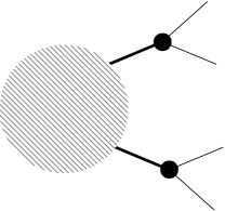
Figure 3: NNLO-type topologies: ${\bf 2}$ (left panel) and ${\bf 1}\!\otimes\!{\bf 1}$ (right panel).

The necessity of introducing the notion of topology emerges at NNLO even without considering the soft limits and the problem of overlapping divergences, as is clear by inspection of the purely collinear limits, eqs. (36) and (37). These are associated with the branching processes depicted in fig. 3; we denote the corresponding topologies by ${\bf 2}$ and ${\bf 1}\!\otimes\!{\bf 1}$ respectively (again, this notation serves as a reminder of the number of partons to be removed from the list of resolved partons). Some of the singular limits in which one or two partons are soft cannot be straightforwardly associated with either topology. However, as in the case of NLO computations, this can be done after some formal manipulations, whose nature (be either a partition of the phase space, or a partial fractioning, or something else) we do not need to specify at this stage. Suffice here to say that, after such manipulations, all singular limits in eqs. (34)–(43) that feature at least one soft parton will in general contribute to both ${\bf 2}$ and ${\bf 1}\!\otimes\!{\bf 1}$ topologies (we may formally write, for example, $f(SS)=f(SS^{({\bf 2})})+f(SS^{({\bf 1}\!\otimes\!{\bf 1})})$). The same kind of procedure can be applied to the singular limits of eqs. (4)–(6), since topology ${\bf 1}$ can always be seen as a sub-topology of ${\bf 2}$ or ${\bf 1}\!\otimes\!{\bf 1}$; thus, $S$, $C$, and $SC$ limits will be manipulated, if need be, so as to be associated with topologies ${\bf 2}$ and ${\bf 1}\!\otimes\!{\bf 1}$. In the case we shall need to distinguish between the singular limits in the various topologies, we shall denote them by $L^{({\cal T})}$, with ${\cal T}={\bf 1},{\bf 2},{\bf 1}\!\otimes\!{\bf 1}$. However, as for parton labels, topology labels may be understood in what follows.

We now claim that by applying the ${\cal E}$-prescription defined in sect. 2 we can systematically subtract the singularities of the double-real contribution to the NNLO cross section, provided that the operator ${\cal E}_{\scriptscriptstyle NLO}$ is replaced by ${\cal E}_{\scriptscriptstyle NNLO}$, where

$${\cal E}_{\scriptscriptstyle NNLO}(f) = {\cal E}_{\scriptscriptstyle NLO}(f)-\sum_{{\cal T}={\bf 2},{\bf 1}\!\otimes\!{\bf 1}}\sum_{\alpha}\Bigg{\{}f\left(SC_{\alpha}^{({\cal T})}\right)+f\left(SS_{\alpha}^{({\cal T})}\right)+f\left(CC_{\alpha}^{({\cal T})}\right)$$ (44)

$$\phantom{\sum_{{\cal T}={\bf 2},{\bf 1}\!\otimes\!{\bf 1}}\sum_{\alpha}}+f\left(SSC_{\alpha}^{({\cal T})}\right)+f\left(SCC_{\alpha}^{({\cal T})}\right)+f\left(SSCC_{\alpha}^{({\cal T})}\right)\Bigg{\}},$$

and $\alpha$ denotes all indices relevant to the corresponding singular limits, which can be read in eqs. (36)–(43). As in the case of NLO computations, the iterative ${\cal E}$-prescription comes to an end thanks to the infrared safety of the observables. However, at NNLO up to four iterations are necessary in order to define $\tilde{f}$, which can be easily generated by means of an algebraic-manipulation code. In such a way, one obtains up to 51 terms for each topology; fortunately, such a massive counterterm can be greatly simplified. We start by observing that the freedom in the definition of the asymptotic form of the matrix elements associated with a given singular limit allows us to exploit commutation properties as done in eq. (13). Furthermore, the presence of ${\cal E}_{\scriptscriptstyle NLO}$ in the definition of ${\cal E}_{\scriptscriptstyle NNLO}$ implies that some of the terms obtained with the ${\cal E}$-prescription will be formally identical to those appearing in an NLO subtraction. This suggests us to write

$$\tilde{f}=\tilde{f}_{-1}+\tilde{f}_{-2}^{({\bf 2})}+\tilde{f}_{-2}^{({\bf 1}\!\otimes\!{\bf 1})}\,,$$ (45)

where

$$\tilde{f}_{-1}=\sum_{i}f\left(S_{i}^{({\bf 1})}\right)+\sum_{i<j}f\left(C_{ij}^{({\bf 1})}\right)-\sum_{ij}f\left(SC_{ij}^{({\bf 1})}\right),$$ (46)

and

$$\tilde{f}_{-2}^{({\cal T})} = \sum_{\alpha}\Bigg{\{}f\left(CC_{\alpha}^{({\cal T})}\right)+f\left(SS_{\alpha}^{({\cal T})}\right)-f\left(SC_{\alpha}^{({\cal T})}\right)-f\left([C\oplus SS]_{\alpha}^{({\cal T})}\right)$$ (47)

$$\phantom{\sum_{\alpha}}-f\left([CC\oplus S]_{\alpha}^{({\cal T})}\right)-f\left([CC\oplus SS]_{\alpha}^{({\cal T})}\right)-f\left([S\oplus S]_{\alpha}^{({\cal T})}\right)-f\left([C\oplus C]_{\alpha}^{({\cal T})}\right)$$

$$\phantom{\sum_{\alpha}}+f\left([C\oplus S\oplus S]_{\alpha}^{({\cal T})}\right)+f\left([CC\oplus S\oplus S]_{\alpha}^{({\cal T})}\right)+f\left([C\oplus C\oplus S]_{\alpha}^{({\cal T})}\right)$$

$$\phantom{\sum_{\alpha}}+f\left([C\oplus C\oplus SS]_{\alpha}^{({\cal T})}\right)-f\left([C\oplus C\oplus S\oplus S]_{\alpha}^{({\cal T})}\right)\Bigg{\}},$$

where we used the fact that (for example) $SSC=SS\oplus C=C\oplus SS$, and $\alpha$ denotes symbolically the relevant parton indices, not indicated explicitly in order to simplify the notation. The physical meaning of eqs. (45)–(47) is clear: in the double real contribution to an NNLO cross section, there are terms with one or two unresolved partons. The former have the same kinematics as those relevant to a pure NLO subtraction. More interestingly, they also have the same kinematics as the real-virtual contribution. Although this fact formally results from the application of the ${\cal E}$-prescription, it can also be understood intuitively: by requiring more stringent jet-finding conditions (for example, by enlarging the minimum $p_{\scriptscriptstyle T}$ which defines a tagged jet), the NNLO cross section turns into an NLO one, which receives contributions only from the real-virtual term, and from the pieces obtained by applying ${\cal E}_{\scriptscriptstyle NLO}$ to the double-real matrix elements. Clearly, if $f$ is associated with an $(n+2)$-body final state, each term in $\tilde{f}_{-1}$ and $\tilde{f}_{-2}$ factorize $(n+1)$-body and $n$-body hard matrix elements and measurement functions respectively.

In order to give more details on the structure of the subtraction that emerges from the ${\cal E}$-prescription, let us denote by

$$vv = g_{\scriptscriptstyle S}^{2n}\left(\left|{\cal M}_{n}^{(1)}\right|^{2}+{\cal M}_{n}^{(0)}{\cal M}_{n}^{(2)^{\star}}+{\cal M}_{n}^{(0)^{\star}}{\cal M}_{n}^{(2)}\right),$$ (48)

$$rv = g_{\scriptscriptstyle S}^{2n}\left({\cal M}_{n+1}^{(0)}{\cal M}_{n+1}^{(1)^{\star}}+{\cal M}_{n+1}^{(0)^{\star}}{\cal M}_{n+1}^{(1)}\right),$$ (49)

$$rr = g_{\scriptscriptstyle S}^{2n}\left|{\cal M}_{n+2}^{(0)}\right|^{2},$$ (50)

the double-virtual, real-virtual, and double-real matrix elements squared respectively, possibly times measurement functions that we understand. The jet cross section is

$$d\sigma = d\sigma_{rr}+d\sigma_{rv}+d\sigma_{vv}$$ (51)

$$= \int rrd\Phi_{n+2}+\int rvd\Phi_{n+1}+\int vvd\Phi_{n}\,.$$ (52)

We start by applying the ${\cal E}$-prescription to the double-real contribution

$$d\sigma_{rr}=\int\left(rrd\Phi_{n+2}-\widetilde{rr}_{\!-2}d\tilde{\Phi}_{n+2}^{-2}-\widetilde{rr}_{\!-1}d\tilde{\Phi}_{n+2}^{-1}\right)+\int\widetilde{rr}_{\!-2}d\tilde{\Phi}_{n+2}^{-2}+\int\widetilde{rr}_{\!-1}d\tilde{\Phi}_{n+2}^{-1},$$ (53)

where we allowed the possibility of adopting two different parametrizations for the phase spaces attached to $\widetilde{rr}_{\!-2}$ and to $\widetilde{rr}_{\!-1}$. The first integral on the r.h.s. of eq. (53) is finite, and can be computed numerically after removing the regularization by letting $\epsilon\to 0$. The second and the third integrals will contain all the divergences of the double-real contribution, to be cancelled by those of the real-virtual and double-virtual contributions. However, only the second term can, at this stage, be integrated analytically. In fact, $\widetilde{rr}_{\!-1}$ is, according to its definition, obtained by considering the asymptotic behaviour of the double-real matrix element squared in the singular limits $S$, $C$, and $SC$ of NLO nature. These limits will render manifest only part of the singular structure of the matrix elements, preventing a complete analytical integration of the divergent terms. For example, if parton $i$ becomes soft, $rr(S_{i})$ factors the eikonal term of eq. (16), and the integration over the variables of parton $i$ can be carried out analytically, as in the case of NLO. However, at NNLO we must take into account that another singularity may appear – say, parton $l$ may also become soft, and $rr(S_{i})$ has too complicated a dependence upon the variables of parton $l$ to perform the necessary analytical integration. Notice that this is not true for, say, $rr(SS_{il})$, which is why the second term on the r.h.s. of eq. (53) can indeed be integrated. This suggests combining $\widetilde{rr}_{\!-1}$ with the real-virtual contribution which, as discussed in sect. 3.1, cannot be integrated analytically too (although for different reasons). In order to achieve this combination, we must choose the phase-space measure appropriately; in particular, we shall use

$$d\tilde{\Phi}_{n+2}^{-1}=d\Phi_{n+1}d\Phi_{2}^{-1}\,,$$ (54)

where $d\Phi_{n+1}$ is the exact $(n+1)$-body massless phase space, and $d\Phi_{2}^{-1}$ is related to the phase space relevant to the partons whose contributions to the singular behaviour of the double-real matrix elements is explicit in $\widetilde{rr}_{\!-1}$, and includes the measure over the virtuality of the branching parton; we shall show in what follows how to construct explicitly the phase spaces of eq. (54). Having done that, we define a subtracted real-virtual contribution as follows

$$rv^{(s)}=rv+\int\widetilde{rr}_{\!-1}d\Phi_{2}^{-1}\,.$$ (55)

In an NLO computation, eq. (55) would amount to the full NLO correction, with the first and the second term on the r.h.s. playing the roles of virtual and real contributions respectively. This implies that the explicit poles in $1/\epsilon$ that appear in $rv$ because of the loop integration will be exactly cancelled by those of $\widetilde{rr}_{\!-1}$ which result from the phase-space integration $d\Phi_{2}^{-1}$. Thus, although in an NNLO computation $rv^{(s)}$ still contains phase-space divergences, we can manipulate it in the same manner as a real contribution to an NLO cross section:

$$\int rv^{(s)}d\Phi_{n+1}=\int\left(rv^{(s)}d\Phi_{n+1}-\widetilde{rv}^{(s)}d\tilde{\Phi}_{n+1}\right)+\int\widetilde{rv}^{(s)}d\tilde{\Phi}_{n+1}\,.$$ (56)

The last term on the r.h.s. of eq. (56) can now be integrated analytically, whereas the first is finite and can be integrated numerically. Therefore, by combining part of the double-real and the real-virtual contributions we have managed to define a scheme in which the analytical integration of all the divergent terms is possible. By combining eqs. (52), (53), and (56) we get

$$d\sigma = \int\left(rrd\Phi_{n+2}-\widetilde{rr}_{\!-2}d\tilde{\Phi}_{n+2}^{-2}-\widetilde{rr}_{\!-1}d\tilde{\Phi}_{n+2}^{-1}\right)$$ (57)

$$+ \int\left(rv^{(s)}d\Phi_{n+1}-\widetilde{rv}^{(s)}d\tilde{\Phi}_{n+1}\right)$$

$$+ \int\widetilde{rr}_{\!-2}d\tilde{\Phi}_{n+2}^{-2}+\int\widetilde{rv}^{(s)}d\tilde{\Phi}_{n+1}+\int vvd\Phi_{n}\,,$$

where the first two terms on the r.h.s. are finite, and can be integrated numerically after letting $\epsilon\to 0$; the sum of the remaining terms is also finite, but they are individually divergent and must be computed analytically.

In order to show explicitly how our master subtraction formula eq. (57) works, we consider the unphysical case in which only singular limits of collinear nature can contribute to the cross section. In such a situation, the application of the ${\cal E}$-prescription is trivial, and we readily arrive at:

$$\widetilde{rr}_{\!-2}\,d\tilde{\Phi}_{n+2}^{-2}=rr(CC)\,d\tilde{\Phi}_{n+2}^{-2}(CC)-rr(C\oplus C)\,d\tilde{\Phi}_{n+2}^{-2}(C\oplus C)\,,$$ (58)

$$\widetilde{rr}_{\!-1}\,d\tilde{\Phi}_{n+2}^{-1}=rr(C)\,d\tilde{\Phi}_{n+2}^{-1}(C)\,.$$ (59)

As in the general formula for the subtraction counterterm at NLO, eq. (15), we leave the possibility open of associating different phase spaces measures with different terms in $\widetilde{rr}_{\!-2}$. This has the advantage that each parametrization can be tailored in order to simplify as much as possible the analytical integration. The drawback is that, in general, there could be algebraic simplifications among the contributions to $\widetilde{rr}_{\!-2}$ (here, between $rr(CC)$ and $rr(C\oplus C)$), which can be explicitly carried out only upon factorizing the phase space. We shall discuss this point further in the following, in the context of a more physical case.

By construction, $rr(C\oplus C)$ is the strongly-ordered, double-collinear limit. This may coincide with $rr(CC)$, and it does in particular in topology ${\bf 1}\!\otimes\!{\bf 1}$, but in general $\widetilde{rr}_{\!-2}$ is different from zero, and corresponds to the non-strongly-ordered part of the double-collinear limit. As such, when a kinematic configuration is generated in which two, and only two partons are collinear, we have $\widetilde{rr}_{\!-2}\to 0$; in other words, the $C$ limit of $\widetilde{rr}_{\!-2}$ is zero. This is what should happen: in the collinear limit, $rr(C)$ (which appears in $\widetilde{rr}_{\!-1}$) is sufficient to cancel locally the divergences of $rr$, and thus $\widetilde{rr}_{\!-2}$ should not diverge in this limit, since otherwise the first term on the r.h.s. of eq. (57) would not be finite. Analogously, in the double-collinear limit the local counterterm for $rr$ is $rr(CC)$; therefore, in order to avoid divergences, in such a limit the contribution of $rr(C\oplus C)$ (in $\widetilde{rr}_{\!-2}$) must cancel that of $rr(C)$ (in $\widetilde{rr}_{\!-1}$). Notice that, for these cancellations to happen not only at the level of matrix elements, but also at the level of cross sections, suitable choices of the phase spaces must be made. The $C$ limit thus relates $d\tilde{\Phi}_{n+2}^{-2}(CC)$ to $d\tilde{\Phi}_{n+2}^{-2}(C\oplus C)$, whereas the $CC$ limit relates $d\tilde{\Phi}_{n+2}^{-2}(C\oplus C)$ to $d\tilde{\Phi}_{n+2}^{-1}(C)$. A suitable choice in the former case clearly includes the trivial one, where the two phase spaces are taken to be identical.

We finally note that the subtraction formula of eq. (57) appears in a very similar form in ref. [21], where a first discussion was given on the extension of the subtraction method to NNLO. Ref. [21] constructs the NNLO subtraction formula building upon the NLO dipole subtraction [9], and provides the explicit expressions of the NNLO counterterms for the leading-colour contribution to $e^{+}e^{-}\to 2~{}{\rm jets}$. Ref. [21], however, does not discuss the way in which the subtraction kernels can be constructed for more general processes. In our approach, the ${\cal E}$-prescription provides a general framework for the construction of the counterterms $\widetilde{rr}_{\!-1}$, $\widetilde{rr}_{\!-2}$ and $\widetilde{rv}^{(s)}$, and explicitly suggests the subtractions of eq. (57). We find it reassuring that we arrive at a subtraction structure consistent with that of ref. [21], given the fact that neither here nor in ref. [21] a formal proof is given that eq. (57) achieves a complete cancellation of the infrared singularities. We do obtain such a cancellation explicitly, for the $C_{\scriptscriptstyle F}T_{\scriptscriptstyle R}$ colour factor of the dijet cross section, as we shall show in the next section. On the other hand, to the best of our knowledge the counterterms presented in ref. [21] have not yet been integrated over the corresponding phase spaces.

4 An application: the $C_{\scriptscriptstyle F}T_{\scriptscriptstyle R}$ part of $e^{+}e^{-}\to 2$ jets

In this section, we shall apply the subtraction procedure discussed in sect. 3 to a physical case, namely the contribution proportional to the colour factor $C_{\scriptscriptstyle F}T_{\scriptscriptstyle R}$ of the dijet cross section in $e^{+}e^{-}$ collisions. This is a relatively simple part of the complete calculation of an observable to NNLO, but it allows us to discuss the practical implementation of most of the features of the subtraction procedure we propose in this paper. The branching kernels that we shall introduce are universal, i.e. they can be used in any other computations where they are relevant. We shall also define precisely the phase spaces needed to integrate the above kernels over the variables of unresolved partons, i.e. the quantities $d\tilde{\Phi}$ used in the formal manipulations of sect. 3. We shall show that the subtraction procedure leads to the expected KLN cancellation, and that the numerical integration of the finite remainder gives a result in excellent agreement with that obtained in ref. [19].

Although not necessary for the implementation of eq. (57), in this section we shall use partial fractioning to deal with the eikonal factors associated with soft singularities, and combine them with the corresponding collinear factors by using the same kinematics in the hard matrix elements that factorize. Since such kinematics will also enter the measurement functions appearing in the counterterms, all of the manipulations involving the hard matrix elements will also apply to the measurement functions; for this reason, the latter will be left implicit in the notation.

We shall reinstate here the notation commonly used for QCD amplitudes, which can be written as vectors in a colour space including the coupling constant. Thus, eq. (30) is now rewritten as

$$|{\cal M}_{a_{1}a_{2}\dots a_{m}}\rangle=|{\cal M}^{(0)}_{a_{1}a_{2}\dots a_{m}}\rangle+|{\cal M}^{(1)}_{a_{1}a_{2}\dots a_{m}}\rangle+|{\cal M}^{(2)}_{a_{1}a_{2}\dots a_{m}}\rangle+\dots$$ (60)

where ${a_{1}a_{2}\dots a_{m}}$ are flavour indices, and particles other than QCD partons are always understood. When not necessary, flavour labels and colour vector symbols may also be understood.

UV renormalization is performed in the ${\overline{\rm MS}}$ scheme, just by expressing the bare coupling $\alpha_{\scriptscriptstyle S}^{u}$ in terms of the renormalized coupling $\alpha_{\scriptscriptstyle S}(\mu^{2})$ at the renormalization scale $\mu$. We use the following expression

$$\alpha_{\scriptscriptstyle S}^{u}\,\mu_{0}^{2\epsilon}\,S_{\epsilon}=\alpha_{\scriptscriptstyle S}(\mu^{2})\,\mu^{2\epsilon}\left[1-\frac{\alpha_{\scriptscriptstyle S}(\mu^{2})}{2\pi}\;\frac{\beta_{0}}{\epsilon}+\dots\right]\,,$$ (61)

where $\beta_{0}=\frac{11}{6}C_{\scriptscriptstyle A}-\frac{2}{3}n_{\scriptscriptstyle F}T_{\scriptscriptstyle R}$, and

$$S_{\epsilon}=(4\pi)^{\epsilon}e^{-\epsilon\gamma_{\scriptscriptstyle E}}$$ (62)

is the typical phase space factor in $d=4-2\epsilon$ dimensions ($\gamma_{\scriptscriptstyle E}=0.5772...$ being the Euler number).

Figure 4: Sample diagrams for double-real (left panel) and real-virtual (right panel) contributions to the $C_{\scriptscriptstyle F}T_{\scriptscriptstyle R}$ part of the dijet cross section.

The diagrams contributing to the $C_{\scriptscriptstyle F}T_{\scriptscriptstyle R}$ part of ${\cal M}^{(0)}_{4}$ (i.e., to the double real) are of the kind of that displayed in the left panel of fig. 4; thus, the singular limits we are interested in are associated with the branchings $g\to q\bar{q}$ and $q\to qq^{\prime}\bar{q}^{\prime}$ (the identical-flavour branching $q\to qq\bar{q}$ is also accounted for by considering $q\to qq^{\prime}\bar{q}^{\prime}$, since its interference contributions are not proportional to $C_{\scriptscriptstyle F}T_{\scriptscriptstyle R}$). As far as the real-virtual contribution is concerned, a sample diagram of ${\cal M}^{(1)}_{3}$ is depicted in the right panel of fig. 4; the singular limits of phase-space origin which, according to the discussion given in sect. 3.2, are obtained upon applying the ${\cal E}$-prescription, are associated with the branching $q\to qg$.

4.1 The double-real contribution

Thanks to the universality properties of soft and collinear emissions, any matrix element with singularities due to the branchings $g\to q\bar{q}$ and $q\to qq^{\prime}\bar{q}^{\prime}$ can be used to define the subtraction terms relevant to the double-real contribution. Thus, we write the double-real matrix element squared as

$$rr=\langle{\cal M}^{(0)}_{q^{\prime}_{1}\bar{q}^{\prime}_{2}q_{3}\dots a_{n+2}}|{\cal M}^{(0)}_{q^{\prime}_{1}\bar{q}^{\prime}_{2}q_{3}\dots a_{n+2}}\rangle\,,$$ (63)

where the labels imply that the four-momenta of $q^{\prime}$, $\bar{q}^{\prime}$ and $q$ are $k_{1}$, $k_{2}$ and $k_{3}$ respectively. When applying the ${\cal E}$-prescription to eq. (63) we obtain from eqs. (46) and (47)

$$\widetilde{rr}_{\!-2} = rr(CC)+rr(SS)-rr(CC\oplus SS)$$ (64)

$$- rr(C\oplus C)-rr(C\oplus SS)+rr(C\oplus C\oplus SS)\,,$$

$$\widetilde{rr}_{\!-1} = rr(C)\,,$$ (65)

where clearly $C\equiv C_{12}$, $CC\equiv CC_{123}$, and so forth. In order to compute explicitly the quantities that appear in eqs. (64) and (65), we shall use the results of ref. [33] (see also refs. [32, 34]). The asymptotic behaviours obtained through successive iterations of ${\cal E}_{\scriptscriptstyle NNLO}$, characterized by the $\oplus$ symbol, can be freely defined to a certain extent. We give such definitions within a given parametrization of the phase space, which we shall introduce in the next subsection.

4.1.1 Choices of phase spaces

As discussed in sect. 3.2 (see in particular eq. (53)), the definition of the double-real subtraction terms implies the necessity of defining $d\tilde{\Phi}_{n+2}^{-2}$ and $d\tilde{\Phi}_{n+2}^{-1}$ which are related to some extent. As a preliminary step, we make here the choice of associating the same $d\tilde{\Phi}_{n+2}^{-2}$ with all of the terms that appear in eq. (64); this is in principle not necessary (see eq. (58)), but we find it non restrictive in the computations that follow (more complicated kernels may require a different choice). We then write the exact $(n+2)$-body phase space using eq. (156)

$$d\Phi_{n+2}=\frac{ds_{123}}{2\pi}\,d\Phi_{n}(123)\,d\Phi_{3}(1,2,3)\,,$$ (66)

where we use the momenta labels rather than the four-momenta to shorten the notation (consistently with eq. (18), $123$ means $k_{1}+k_{2}+k_{3}$), and

$$s_{123}=(k_{1}+k_{2}+k_{3})^{2}\,.$$ (67)

As in the case of NLO computations, eq. (66) is unsuited for the analytical integration over the variables of unresolved partons since $123$, which enters the phase space associated with the non-singular part of the matrix element, has an off-shellness $s_{123}$, while the reduced matrix element which corresponds to such non-singular part has all of the final-state QCD partons with zero mass. We follow the same strategy as in eq. (19), i.e. that of ref. [8]: we introduce a four-momentum $\widetilde{123}$ with invariant mass equal to zero, and define

$$d\tilde{\Phi}_{n+2}^{-2}=d\Phi_{n}(\widetilde{123})\,\frac{ds_{123}}{2\pi}\,d\Phi_{3}(1,2,3)\,.$$ (68)

This definition is equivalent to that in eq. (19), and differs from that in eq. (24) in that no spectator is used to keep the branching parton on shell.

For the definition of $d\tilde{\Phi}_{n+2}^{-1}$, we use again eq. (156)

$$d\Phi_{n+2}=\frac{ds_{12}}{2\pi}\,d\Phi_{n+1}(12)\,d\Phi_{2}(1,2)\,,$$ (69)

from which the analogue of eq. (68) can readily follow:

$$d\tilde{\Phi}_{n+2}^{-1}=d\Phi_{n+1}(\widetilde{12})\,\frac{ds_{12}}{2\pi}\,d\Phi_{2}(1,2)\,.$$ (70)

There is however a subtlety: as discussed in sect. 3.2, the choice of $d\tilde{\Phi}_{n+2}^{-1}$ must match that of $d\tilde{\Phi}_{n+2}^{-2}$. In order to see how this can happen, we use eq. (167) to write

$$d\tilde{\Phi}_{n+2}^{-2}=d\Phi_{n}(\widetilde{123})\,\frac{ds_{123}}{2\pi}\,\frac{ds_{12}}{2\pi}\,d\Phi_{2}(3,12)\,d\Phi_{2}(1,2)\,.$$ (71)

The part relevant to the $12\to 1+2$ branching is identical in eqs. (70) and (71), except for the fact that the invariant mass of the $12$ system, $s_{12}$, enters $d\Phi_{2}(3,12)$, and not only $d\Phi_{2}(1,2)$, in eq. (71). If this dependence could be safely neglected in the limit $s_{12}\to 0$, i.e. in the singular region in which $d\tilde{\Phi}_{n+2}^{-1}$ and $d\tilde{\Phi}_{n+2}^{-2}$ must match, the choice of eq. (70) would be appropriate. However, as can be seen from eqs. (170) and (172), $d\Phi_{2}(3,12)$ contains the factor

$$\left(z_{3}z_{12}s_{123}-z_{3}s_{12}\right)^{-\epsilon}\,,$$ (72)

which acts as a regulator in the integrations in $d\Phi_{2}(3,12)$; since these are in general divergent, the regulator affects finite (and possibly also divergent) terms, and thus cannot be ignored even if the limit $s_{12}\to 0$ is considered. The regulator of eq. (72) is implicit in $d\Phi_{n+1}(12)$ in eq. (69); the effect of neglecting it as done by defining $d\tilde{\Phi}_{n+2}^{-1}$ in eq. (69) therefore leads to neglecting contributions to the cross section if $d\Phi_{n+1}(\widetilde{12})$ is involved in the integration of divergent terms. This is what happens, since the subtracted real-virtual contribution is indeed divergent. This problem may seem to be cured by inserting the regulator of eq. (72) into the r.h.s. of eq. (70). However, the definition of $d\tilde{\Phi}_{n+2}^{-1}$ should not depend on whether the branching $12\to 1+2$ is followed by the branching $123\to 3+12$, which is what the presence of $s_{123}$ in eq. (72) implies. The most general form for the regulator to be inserted in eq. (70) can be deduced by writing

$$d\Phi_{n+2}=\frac{ds_{12}}{2\pi}\,\frac{ds_{3\dots(n+2)}}{2\pi}\,d\Phi_{2}(12,3\dots(n+2))\,d\Phi_{2}(1,2)\,d\Phi_{n}(3,\dots,(n+2))\,.$$ (73)

The first phase space on the r.h.s. features the regulator

$$\left(z_{12}z_{3\dots(n+2)}Q^{2}-z_{12}s_{3\dots(n+2)}-z_{3\dots(n+2)}s_{12}\right)^{-\epsilon}\equiv\left(z_{3\dots(n+2)}s_{12}^{\rm max}\right)^{-\epsilon}\left(1-\frac{s_{12}}{s_{12}^{\rm max}}\right)^{-\epsilon}\,,$$ (74)

which can be obtained from eqs. (162) and (163), and where

$$s_{12}^{\rm max}=\left(z_{12}z_{3\dots(n+2)}Q^{2}-z_{12}s_{3\dots(n+2)}\right)/z_{3\dots(n+2)}\,,$$ (75)

with $Q^{2}=(k_{1}+\dots+k_{n+2})^{2}$. Eq. (74) suggests to replace eq. (70) with

$$d\tilde{\Phi}_{n+2}^{-1}=d\Phi_{n+1}(\widetilde{12})\,\frac{ds_{12}}{2\pi}\,\left(1-\frac{s_{12}}{s_{12}^{\rm max}}\right)^{-\epsilon}d\Phi_{2}(1,2)\,,$$ (76)

where the quantity $s_{12}^{\rm max}$ is a constant with respect to the integration in $s_{12}$.

4.1.2 Computation of the divergent terms

In this section, we integrate $\widetilde{rr}_{\!-2}$ and $\widetilde{rr}_{\!-1}$ given in eqs. (64) and (65) over the phase spaces defined in sect. 4.1.1. We start from the case of $\widetilde{rr}_{\!-2}$, and write

$$\widetilde{rr}_{\!-2}=\langle{\cal M}^{(0)}_{q\dots a_{n+2}}|{{\mbox{\boldmath$K$}}}^{(3)}_{q^{\prime}_{1}\bar{q}^{\prime}_{2}q_{3}}|{\cal M}^{(0)}_{q\dots a_{n+2}}\rangle\,.$$ (77)

The kernel ${{\mbox{\boldmath$K$}}}^{(3)}_{q^{\prime}_{1}\bar{q}^{\prime}_{2}q_{3}}$ is a matrix in the colour space, and collects all singular behaviours associated with the branching $q\to q^{\prime}_{1}\bar{q}^{\prime}_{2}q_{3}$ according to the combination given in eq. (64). For its explicit construction we shall use the factorization formulae given in ref. [33]. In general, we shall denote the branching kernels as follows

$${{\mbox{\boldmath$K$}}}^{(n)}_{a_{1}\dots a_{n}}\;\;\;\;\;\;{\rm for}\;\;\;\;\;\;S(a_{1},\dots,a_{n})\to a_{1}+\dots+a_{n}\,,$$ (78)

where $S(a_{1},\dots,a_{n})$ is the parton flavour which matches the combination $a_{1}+\dots+a_{n}$. In this paper, only $n=2,3$ will be considered. Notice that the notation of eq. (78) does not coincide with the one typically used for two-parton branchings, where the Altarelli-Parisi kernel is denoted by $P_{a_{1}S(a_{1},a_{2})}$. There is a remarkable simplification that occurs in the computation of eq. (77); namely, one can prove that (see app. A)

$$rr(SS)=rr(C\oplus SS)\,,\;\;\;\;\;\;\;\;rr(CC\oplus SS)=rr(C\oplus C\oplus SS)\,.$$ (79)

Thus

$$\widetilde{rr}_{\!-2}=rr(CC)-rr(C\oplus C)\,.$$ (80)

Since in the collinear limits colour correlations do not appear, eq. (80) implies that ${{\mbox{\boldmath$K$}}}^{(3)}_{q^{\prime}_{1}\bar{q}^{\prime}_{2}q_{3}}$ has a trivial structure in colour space. Using the same normalization in the factorization formulae as in ref. [33] (see eq. (29) there), we thus rewrite the kernel as follows

$${{\mbox{\boldmath$K$}}}^{(3)}_{q^{\prime}_{1}\bar{q}^{\prime}_{2}q_{3}}=\frac{(8\pi\alpha_{\scriptscriptstyle S}^{u}\mu_{0}^{2\epsilon})^{2}}{s_{123}^{2}}\left(K_{q^{\prime}_{1}\bar{q}^{\prime}_{2}q_{3}}^{CC}-K_{q^{\prime}_{1}\bar{q}^{\prime}_{2}q_{3}}^{C\oplus C}\right)\,,$$ (81)

where the first term can be read from eq. (57) of ref. [33]

$$K_{q^{\prime}_{1}\bar{q}^{\prime}_{2}q_{3}}^{CC}=\frac{1}{2}\,C_{\scriptscriptstyle F}T_{\scriptscriptstyle R}\,\frac{s_{123}}{s_{12}}\Bigg{[}-\frac{t_{12,3}^{2}}{s_{12}s_{123}}+\frac{4z_{3}+(z_{1}-z_{2})^{2}}{z_{1}+z_{2}}+(1-2\epsilon)\left(z_{1}+z_{2}-\frac{s_{12}}{s_{123}}\right)\Bigg{]}\,,$$ (82)

and

$$t_{ij,k}\equiv 2\;\frac{z_{i}s_{jk}-z_{j}s_{ik}}{z_{i}+z_{j}}+\frac{z_{i}-z_{j}}{z_{i}+z_{j}}\,s_{ij}\,.$$ (83)

The quantity $K_{q^{\prime}_{1}\bar{q}^{\prime}_{2}q_{3}}^{C\oplus C}$ in eq. (81) corresponds to the successive branchings $q\to q_{3}g$, $g\to q^{\prime}_{1}\bar{q}^{\prime}_{2}$. We can therefore construct it by using the polarized Altarelli-Parisi kernels ${\hat{P}}_{gq}^{\mu\nu}$ and ${\hat{P}}_{q\bar{q}}^{\mu\nu}$, as shown in app. A. The result is

$$K^{C\oplus C}_{q^{\prime}_{1}\bar{q}^{\prime}_{2}q_{3}}=\frac{1}{2}\,C_{\scriptscriptstyle F}T_{\scriptscriptstyle R}\,\frac{s_{123}}{s_{12}}\Bigg{[}-\frac{t_{12,3}^{(S)^{2}}}{s_{12}s_{123}}+\frac{4z_{3}+(z_{1}-z_{2})^{2}}{z_{1}+z_{2}}+(1-2\epsilon)\left(z_{1}+z_{2}\right)\Bigg{]}\,,$$ (84)

where

$$t_{ij,k}^{(S)}\equiv 2\;\frac{z_{i}s_{jk}-z_{j}s_{ik}}{z_{i}+z_{j}}\,.$$ (85)

We note that the result in eq. (84) corresponds to the naive $s_{12}\to 0$ limit of $K_{q^{\prime}_{1}\bar{q}^{\prime}_{2}q_{3}}^{CC}$ in eq. (82), since $t_{12,3}\to t_{12,3}^{(S)}\propto\sqrt{s_{12}}$ in such a limit (see app. B). The kernel ${{\mbox{\boldmath$K$}}}^{(3)}_{q^{\prime}_{1}\bar{q}^{\prime}_{2}q_{3}}$ is therefore manifestly simpler than its two contributions in eq. (81); using the results of eqs. (82) and (84), we find

$${{\mbox{\boldmath$K$}}}^{(3)}_{q^{\prime}_{1}\bar{q}^{\prime}_{2}q_{3}}=\frac{(8\pi\alpha_{\scriptscriptstyle S}^{u}\mu_{0}^{2\epsilon})^{2}}{s_{123}^{2}}\,\frac{1}{2}C_{\scriptscriptstyle F}T_{\scriptscriptstyle R}\frac{s_{123}}{s_{12}}\Bigg{[}-\frac{t_{12,3}^{2}-t_{12,3}^{(S)^{2}}}{s_{12}s_{123}}-(1-2\epsilon)\frac{s_{12}}{s_{123}}\Bigg{]}\,.$$ (86)

We can now obtain the analytical expressions of the $1/\epsilon$ poles in $\widetilde{rr}_{\!-2}$. Using eq. (68)

$$\int\widetilde{rr}_{\!-2}d\tilde{\Phi}_{n+2}^{-2}=\left|{\cal M}^{(0)}_{q\dots a_{n+2}}\right|^{2}d\Phi_{n}\int\frac{ds_{123}}{2\pi}{{\mbox{\boldmath$K$}}}^{(3)}_{q^{\prime}_{1}\bar{q}^{\prime}_{2}q_{3}}\,d\Phi_{3}(1,2,3)\,.$$ (87)

We use the parametrization of eq. (178) to perform the integration in eq. (87). The invariants are expressed in terms of the integration variables according to eqs. (175) and (176); however, one must be careful when replacing these expressions into $t_{12,3}^{(S)}$, since in doing so finite terms are generated when $s_{12}\to 0$; such terms should not appear, since they have been explicitly neglected when working $K^{C\oplus C}_{q^{\prime}_{1}\bar{q}^{\prime}_{2}q_{3}}$ out. To avoid this, we use

$$z_{1}s_{23}-z_{2}s_{13}\to\sqrt{s_{12}}\xi_{0}\,,\;\;\;\;\;\;\;\;\xi_{0}=2\sqrt{z_{3}\zeta_{2}(1-\zeta_{2})s_{123}(1-z_{3})}\,x$$ (88)

in the computation of $t_{12,3}^{(S)}$. In a more general case, the replacements

$$s_{13}\to s_{123}(1-\zeta_{2})\,,\;\;\;\;\;\;\;\;s_{23}=s_{123}\,\zeta_{2}$$ (89)

should also be made. The result of the integral in eq. (87) is

$$\int\frac{ds_{123}}{2\pi}{{\mbox{\boldmath$K$}}}^{(3)}_{q^{\prime}_{1}\bar{q}^{\prime}_{2}q_{3}}\,d\Phi_{3}(1,2,3)=\left(\frac{\alpha_{\scriptscriptstyle S}}{2\pi}\right)^{2}C_{\scriptscriptstyle F}T_{\scriptscriptstyle R}\left(\frac{s_{123}^{{\rm max}}}{\mu^{2}}\right)^{-2\epsilon}\frac{1}{6\epsilon}\left(1+\frac{31}{6}\epsilon\right)+{\cal O(\epsilon)}\,,$$ (90)

where we denoted by $s_{123}^{{\rm max}}$ the upper limit of the integration in $s_{123}$, whose form does not need be specified here; a definite choice will be made in sect. 4.3.

We now turn to the case of $\widetilde{rr}_{\!-1}$, and write the analogue of eq. (77)

$$\widetilde{rr}_{\!-1}=\langle{\cal M}^{(0)}_{gq_{3}\dots a_{n+2}}|{{\mbox{\boldmath$K$}}}^{(2)}_{q^{\prime}_{1}\bar{q}^{\prime}_{2}}|{\cal M}^{(0)}_{gq_{3}\dots a_{n+2}}\rangle\,.$$ (91)

As in the case of ${{\mbox{\boldmath$K$}}}^{(3)}_{q^{\prime}_{1}\bar{q}^{\prime}_{2}q_{3}}$, the kernel ${{\mbox{\boldmath$K$}}}^{(2)}_{q^{\prime}_{1}\bar{q}^{\prime}_{2}}$ is purely collinear (see eq. (65)), and therefore has a trivial colour structure. Using again the factorization formulae with the normalization of ref. [33] (see eq. (7) there), we have

$$\langle\mu|{{\mbox{\boldmath$K$}}}^{(2)}_{q^{\prime}_{1}\bar{q}^{\prime}_{2}}|\nu\rangle=\frac{8\pi\alpha_{\scriptscriptstyle S}^{u}\mu_{0}^{2\epsilon}}{s_{12}}{\hat{P}}_{q\bar{q}}^{\mu\nu}\,,$$ (92)

where ${\hat{P}}_{q\bar{q}}^{\mu\nu}$ is given in eq. (138). Spin correlations are essential for the kernel ${{\mbox{\boldmath$K$}}}^{(2)}$ to be a local subtraction counterterm, but they do not contribute to the analytic integration which follows, where the spin-dependent collinear kernel ${\hat{P}}_{q\bar{q}}^{\mu\nu}$ can be replaced by

$$\langle P_{q\bar{q}}\rangle=T_{\scriptscriptstyle R}\Bigg{[}1-\frac{2z(1-z)}{1-\epsilon}\Bigg{]}\,.$$ (93)

Using eq. (76) we obtain

$$\int\widetilde{rr}_{\!-1}d\tilde{\Phi}_{n+2}^{-1}=\left|{\cal M}^{(0)}_{gq_{3}\dots a_{n+2}}\right|^{2}d\Phi_{n+1}\int\frac{ds_{12}}{2\pi}{{\mbox{\boldmath$K$}}}^{(2)}_{q^{\prime}_{1}\bar{q}^{\prime}_{2}}\left(1-\frac{s_{12}}{s_{12}^{\rm max}}\right)^{-\epsilon}d\Phi_{2}(1,2)\,.$$ (94)

The integral can be performed straightforwardly, with the result

$$\int\frac{ds_{12}}{2\pi}{{\mbox{\boldmath$K$}}}^{(2)}_{q^{\prime}_{1}\bar{q}^{\prime}_{2}}\left(1-\frac{s_{12}}{s_{12}^{\rm max}}\right)^{-\epsilon}d\Phi_{2}(1,2)=\frac{\alpha_{\scriptscriptstyle S}}{2\pi}\,\frac{e^{\epsilon\gamma_{\scriptscriptstyle E}}}{\Gamma(1-\epsilon)}\,\left(\frac{\mu^{2}}{s_{12}^{{\rm max}}}\right)^{\epsilon}T_{\scriptscriptstyle R}\left(-\frac{1}{\epsilon}\right)$$

$$\phantom{aaaaaaaaaaa}\times\Bigg{[}\frac{2}{3}+\frac{10}{9}\epsilon+\left(\frac{56}{27}-\frac{\pi^{2}}{9}\right)\epsilon^{2}+\left(\frac{328}{81}-\frac{5}{27}\pi^{2}-\frac{4}{3}\zeta_{3}\right)\epsilon^{3}\Bigg{]}$$

$$\phantom{aaaaaaaaaaa}\times\left(1-\frac{\pi^{2}}{6}\epsilon^{2}-2\epsilon^{3}\zeta_{3}\right)+{\cal O}(\epsilon^{3})\,,$$ (95)

where all the terms up to ${\cal O}(\epsilon^{2})$ have been kept, since eq. (95) will be used to define the subtracted real-virtual contribution as given in eq. (55), which will generate further poles up to $1/\epsilon^{2}$.

4.2 The real-virtual contribution

In this section, we shall construct the subtracted real-virtual contribution, defined in eq. (55). As discussed there, $rv^{(s)}$ has no explicit $1/\epsilon$ poles, since those resulting from the one-loop integrals contributing to the (unsubtracted) real-virtual contribution $rv$ are cancelled by those of $\widetilde{rr}_{\!-1}$. We can show this explicitly for the $C_{\scriptscriptstyle F}T_{\scriptscriptstyle R}$ part of the $e^{+}e^{-}$ dijet cross section: the contribution of

$$rv=\langle{\cal M}^{(0)}_{gq\bar{q}}|{\cal M}^{(1)}_{gq\bar{q}}\rangle+\langle{\cal M}^{(1)}_{gq\bar{q}}|{\cal M}^{(0)}_{gq\bar{q}}\rangle$$ (96)

to this colour factor is entirely due to the $T_{\scriptscriptstyle R}$ part resulting from UV renormalization:

$$rv|_{T_{\scriptscriptstyle R}}=\frac{\alpha_{\scriptscriptstyle S}}{2\pi}\frac{2}{3}\frac{T_{\scriptscriptstyle R}n_{\scriptscriptstyle F}}{\epsilon}\left|{\cal M}^{(0)}_{gq\bar{q}}\right|^{2}.$$ (97)

By using eqs. (54), (94), and (95), with $gq_{3}\dots a_{n+2}\equiv gq\bar{q}$ and summing over $n_{\scriptscriptstyle F}$ quark flavours, it is apparent that $rv^{(s)}$ is indeed free of explicit $1/\epsilon$ poles:

$$rv^{(s)}d\Phi_{3} \equiv rv|_{T_{\scriptscriptstyle R}}d\Phi_{3}+\sum_{flav}\int\widetilde{rr}_{\!-1}d\tilde{\Phi}_{4}^{-1}=\frac{\alpha_{\scriptscriptstyle S}}{2\pi}\frac{T_{\scriptscriptstyle R}n_{\scriptscriptstyle F}}{\epsilon}\left|{\cal M}^{(0)}_{gq\bar{q}}\right|^{2}\,d\Phi_{3}$$ (98)

$$\times\Bigg{\{}\frac{2}{3}-\left(\frac{\mu^{2}}{s_{12}^{{\rm max}}}\right)^{\epsilon}\,\frac{e^{\epsilon\gamma_{\scriptscriptstyle E}}}{\Gamma(1-\epsilon)}\Bigg{[}\frac{2}{3}+\frac{10}{9}\epsilon+\left(\frac{56}{27}-\frac{\pi^{2}}{9}\right)\epsilon^{2}$$

$$\phantom{\times}+\left(\frac{328}{81}-\frac{5}{27}\pi^{2}-\frac{4}{3}\zeta_{3}\right)\epsilon^{3}\Bigg{]}\left(1-\frac{\pi^{2}}{6}\epsilon^{2}-2\epsilon^{3}\zeta_{3}\right)\Bigg{\}}+{\cal O}(\epsilon^{3})\phantom{aaaaa}$$

$$= -\frac{\alpha_{\scriptscriptstyle S}}{2\pi}\frac{2T_{\scriptscriptstyle R}n_{\scriptscriptstyle F}}{9}\left(5+3\log\left(\frac{\mu^{2}}{s_{12}^{{\rm max}}}\right)\right)\left|{\cal M}^{(0)}_{gq\bar{q}}\right|^{2}\,d\Phi_{3}+{\cal O}(\epsilon)\,.$$ (99)

We underline the presence of $s_{12}^{{\rm max}}$ in eqs. (98) and (99), due to the integration performed in eqs. (94) and (95), and to the choice of phase space of eq. (76). Its specific form depends on the branchings involved in the construction of $\widetilde{rr}_{\!-1}$, and can be read from eq. (75); we shall write it explicitly in the following, after choosing a parametrization for the phase spaces $d\Phi_{n+1}$ and $d\tilde{\Phi}_{n+1}$.

Implicit divergences remain in eq. (98), whose analytic computation requires the definition of the subtraction counterterm $\widetilde{rv}^{(s)}$ which appears in eq. (56). It is clear that these divergences are those of the matrix element ${\cal M}^{(0)}_{gq\bar{q}}$ which factorizes in eq. (98) and thus are due to the branching $q\to qg$. In order to study them with full generality, we consider

$$rv^{(0)}=\langle{\cal M}^{(0)}_{gq\dots a_{n+1}}|{\cal M}^{(0)}_{gq\dots a_{n+1}}\rangle\,,$$ (100)

from which we construct the subtraction counterterm by applying the ${\cal E}$-prescription:

$$\widetilde{rv}^{(0)}=rv^{(0)}(C)+rv^{(0)}(S)-rv^{(0)}(SC).$$ (101)

Clearly, $\widetilde{rv}^{(s)}$ is obtained by multiplying $\widetilde{rv}^{(0)}$ by the r.h.s. of eq. (98), divided by $\left|{\cal M}^{(0)}_{gq\bar{q}}\right|^{2}\,d\Phi_{3}$; the same manipulations can be carried out on the r.h.s. of eq. (99), in this way obtaining the local subtraction counterterm to be used in the numerical computation of the integral that appears in the first term on the r.h.s. of eq. (56), or in the second line on the r.h.s of eq. (57). We stress that eq. (101) coincides with eq. (14), since the subtraction of the phase-space singularities of $rv^{(s)}$ is identical to that performed in the context of an NLO computation. In what follows, similarly to what done in sect. 4.1, we shall choose the same parametrization of the phase space for the three terms on the r.h.s. of eq. (101), whose sum will therefore be essentially identical to one of the dipole kernels of ref. [9]. As before, we shall however not use the dipole parametrization for the phase space, and our integrated kernel will thus be different from that of ref. [9]. We obtain

$$\widetilde{rv}^{(0)}=\langle{\cal M}^{(0)}_{q\dots a_{n+1}}|{{\mbox{\boldmath$K$}}}^{(2)}_{qg}|{\cal M}^{(0)}_{q\dots a_{n+1}}\rangle\,,$$ (102)

where the kernel has now a non-trivial colour structure

$${{\mbox{\boldmath$K$}}}^{(2)}_{qg}=-\frac{8\pi\mu_{0}^{2\epsilon}\alpha_{\scriptscriptstyle S}^{u}}{s_{qg}}\sum_{k\neq q}{\cal V}^{(2)}_{qg,k}\,{{\mbox{\boldmath$T$}}}_{q}\!\cdot\!{{\mbox{\boldmath$T$}}}_{k}\,.$$ (103)

Here

$${\cal V}^{(2)}_{qg,k} = \frac{2p_{q}\!\cdot\!p_{k}}{(p_{q}+p_{k})\!\cdot\!p_{g}}+(1-z)(1-\epsilon),$$ (104)

$$z = \frac{p_{q}\!\cdot\!p_{k}}{(p_{q}+p_{g})\!\cdot\!p_{k}}\,,$$ (105)

and in order to obtain the result in eq. (104) we have decomposed the eikonal factor that appears in $rv^{(0)}(S)$ as shown in eq. (23).

According to our master subtraction formula, eq. (57), we have now to integrate $\widetilde{rv}^{(s)}$ over the phase space, and thus we have to choose a parametrization for $d\tilde{\Phi}_{n+1}$. A possibility is that of using again the form of eq. (76), which with the parton labeling of the case at hand would read as follows

$$d\tilde{\Phi}_{n+1}=d\Phi_{n}(\widetilde{qg})\,\frac{ds_{qg}}{2\pi}\,\left(1-\frac{s_{qg}}{s_{qg}^{\rm max}}\right)^{-\epsilon}d\Phi_{2}(q,g)\,.$$ (106)

On the other hand, the present case is simpler than that discussed in sect. 4.1. The integration of $\widetilde{rv}^{(s)}$ over $d\tilde{\Phi}_{n+1}$ will not be followed by another analytical integration; thus, the regulator that appears explicitly in eq. (106) is not actually necessary. Furthermore, its presence would require the presence of an analogous regulator for $s_{123}$ in eq. (68). Thus, in order to simplify as much as possible the analytic computations, we rather adopt the following form

$$d\tilde{\Phi}_{n+1}=d\Phi_{n}(\widetilde{qg})\,\frac{ds_{qg}}{2\pi}\,d\Phi_{2}(q,g)\,.$$ (107)

Having made this choice, we can deduce the expression of $s_{12}^{{\rm max}}$ from eq. (75):

$$s_{12}^{{\rm max}}=(1-z)s_{qg}\,.$$ (108)

In order to integrate the kernel ${{\mbox{\boldmath$K$}}}^{(2)}_{qg}$ over $ds_{qg}d\Phi_{2}(q,g)$, we use eq. (162), choosing the reference four-vector $n$ there to coincide with $p_{k}$; in such a way, the variable $z_{1}$ of eq. (159) coincides with $z$ of eq. (105). We also define

$$Q_{qgk}^{2}=(p_{q}+p_{g}+p_{k})^{2}\,,$$ (109)

which is treated as a constant during the integration. We obtain

$$\int\widetilde{rv}^{(0)}d\tilde{\Phi}_{n+1} = -\frac{\alpha_{\scriptscriptstyle S}}{2\pi}\,\frac{e^{\epsilon\gamma_{\scriptscriptstyle E}}}{\Gamma(1-\epsilon)}\sum_{k\neq q}\left(\frac{\mu^{2}}{Q_{qgk}^{2}}\right)^{\epsilon}I_{qg,k}^{(A)}$$ (110)

$$\times \langle{\cal M}^{(0)}_{q\dots a_{n+1}}|{{\mbox{\boldmath$T$}}}_{q}\!\cdot\!{{\mbox{\boldmath$T$}}}_{k}|{\cal M}^{(0)}_{q\dots a_{n+1}}\rangle\,d\Phi_{n}\,.$$

In eq. (98) we also need

$$\int\widetilde{rv}^{(0)}\left(\frac{\mu^{2}}{s_{12}^{\rm max}}\right)^{\epsilon}d\tilde{\Phi}_{n+1} = -\frac{\alpha_{\scriptscriptstyle S}}{2\pi}\,\frac{e^{\epsilon\gamma_{\scriptscriptstyle E}}}{\Gamma(1-\epsilon)}\sum_{k\neq q}\left(\frac{\mu^{2}}{Q_{qgk}^{2}}\right)^{\epsilon}I_{qg,k}^{(B)}$$ (111)

$$\times \langle{\cal M}^{(0)}_{q\dots a_{n+1}}|{{\mbox{\boldmath$T$}}}_{q}\!\cdot\!{{\mbox{\boldmath$T$}}}_{k}|{\cal M}^{(0)}_{q\dots a_{n+1}}\rangle\,d\Phi_{n}\,,$$

with $s_{12}^{\rm max}$ given in eq. (108), and

$$\frac{(4\pi)^{\epsilon}}{\Gamma(1-\epsilon)}\left(\frac{\mu^{2}}{Q_{qgk}^{2}}\right)^{\epsilon}I_{qg,k}^{(A)} = 8\pi\mu^{2\epsilon}\int\frac{ds_{qg}}{s_{qg}}\,d\Phi_{2}(q,g)\,{\cal V}^{(2)}_{qg,k}\,,$$ (112)

$$\frac{(4\pi)^{\epsilon}}{\Gamma(1-\epsilon)}\left(\frac{\mu^{2}}{Q_{qgk}^{2}}\right)^{2\epsilon}I_{qg,k}^{(B)} = 8\pi\mu^{2\epsilon}\int\frac{ds_{qg}}{s_{qg}}\,d\Phi_{2}(q,g)\,\left(\frac{\mu^{2}}{s_{12}^{{\rm max}}}\right)^{\epsilon}{\cal V}^{(2)}_{qg,k}\,.$$ (113)

A somewhat lengthy computation returns the following results

$$I_{qg,k}^{(A)} \equiv \int_{0}^{1}dz\int_{0}^{y_{\rm max}}dy\left[\frac{2z(1-y)}{1-z+yz}+(1-z)(1-\epsilon)\right]\left(z(1-z)\right)^{-\epsilon}y^{-1-\epsilon}$$ (114)

$$= \frac{1}{\epsilon^{2}}+\frac{3}{2}\frac{1}{\epsilon}+\frac{7}{2}-\frac{\pi^{2}}{6}-\log(y_{\rm max})\left(\log(y_{\rm max})+\frac{3}{2}\right)-2{\rm Li}_{2}(1-y_{\rm max})$$

$$+ \epsilon\Bigg{[}7-\frac{\pi^{2}}{4}-2\zeta_{3}+\log(y_{\rm max})\left(\frac{\pi^{2}}{3}-\frac{7}{2}\right)-2\log(y_{\rm max}){\rm Li}_{2}(y_{\rm max})$$

$$+\log^{2}(y_{\rm max})\left(\frac{3}{4}-2\log(1-y_{\rm max})+\frac{2}{3}\log(y_{\rm max})\right)$$

$$-2{\rm Li}_{3}(1-y_{\rm max})+2{\rm Li}_{3}\left(\frac{y_{\rm max}-1}{y_{\rm max}}\right)\Bigg{]}+{\cal O}(\epsilon^{2})\,,$$

$$I_{qg,k}^{(B)} \equiv \int_{0}^{1}dz\int_{0}^{y_{\rm max}}dy\left[\frac{2z(1-y)}{1-z+yz}+(1-z)(1-\epsilon)\right]z^{-\epsilon}(1-z)^{-2\epsilon}y^{-1-2\epsilon}$$ (115)

$$= \frac{1}{4\epsilon^{2}}+\frac{3}{4\epsilon}+\frac{21}{8}-\log(y_{\rm max})\left(\frac{3}{2}+\log(y_{\rm max})\right)-2{\rm Li}_{2}(1-y_{\rm max})$$

$$+ \epsilon\Bigg{[}\frac{127}{16}-\frac{\pi^{2}}{4}-\zeta_{3}+\log(y_{\rm max})\left(\frac{\pi^{2}}{3}-\frac{21}{4}\right)-6\log(y_{\rm max}){\rm Li}_{2}(y_{\rm max})$$

$$+\log^{2}(y_{\rm max})\left(\frac{3}{2}-4\log(1-y_{\rm max})+\frac{4}{3}\log(y_{\rm max})\right)$$

$$-2{\rm Li}_{3}(1-y_{\rm max})+4{\rm Li}_{3}\left(\frac{y_{\rm max}-1}{y_{\rm max}}\right)+4{\rm Li}_{3}(y_{\rm max})\Bigg{]}+{\cal O}(\epsilon^{2})\,,$$

where we have introduced the arbitrary parameter $y_{\rm max}$, which defines the upper limit of the $s_{qg}$ integration

$$s_{qg}\leq y_{\rm max}\,Q_{qgk}^{2}\,,\;\;\;\;\;\;\;\;0<y_{\rm max}\leq 1\,.$$ (116)

The physical results must not depend on $y_{\rm max}$, whose variation amounts to changing finite contributions to the subtraction counterterms; whether this condition is fulfilled represents a powerful check on the correctness of the subtraction procedure. The parameter $y_{\rm max}$ is the analogue of the free parameters $\xi_{cut}$, $\delta_{\scriptscriptstyle I}$ and $\delta_{\scriptscriptstyle O}$ of ref. [8].

4.3 Results

In this section, we shall use the results obtained in sects. 4.1 and 4.2 in order to implement our master subtraction formula eq. (57). As a preliminary step, we need the $C_{\scriptscriptstyle F}T_{\scriptscriptstyle R}$ part of the double-virtual contribution

$$vv=\langle{\cal M}^{(0)}_{q\bar{q}}|{\cal M}^{(2)}_{q\bar{q}}\rangle+\langle{\cal M}^{(2)}_{q\bar{q}}|{\cal M}^{(0)}_{q\bar{q}}\rangle\,,$$ (117)

which can be straightforwardly obtained from ref. [39]:

$$vv|_{C_{\scriptscriptstyle F}T_{\scriptscriptstyle R}} = C_{\scriptscriptstyle F}T_{\scriptscriptstyle R}n_{\scriptscriptstyle F}\left(\frac{\alpha_{\scriptscriptstyle S}}{2\pi}\right)^{2}\left|{\cal M}^{(0)}_{q\bar{q}}\right|^{2}$$ (118)

$$\times \Bigg{\{}\left(\frac{Q^{2}}{\mu^{2}}\right)^{-2\epsilon}\Bigg{[}\frac{1}{3\epsilon^{3}}+\frac{14}{9\epsilon^{2}}+\left(\frac{353}{54}-\frac{11}{18}\pi^{2}\right)\frac{1}{\epsilon}+\frac{7541}{324}-\frac{77}{27}\pi^{2}-\frac{26}{9}\zeta_{3}\Bigg{]}$$

$$+\left(\frac{Q^{2}}{\mu^{2}}\right)^{-\epsilon}\Bigg{[}-\frac{4}{3\epsilon^{3}}-\frac{2}{\epsilon^{2}}+\left(\frac{7}{9}\pi^{2}-\frac{16}{3}\right)\frac{1}{\epsilon}-\frac{32}{3}+\frac{7}{6}\pi^{2}+\frac{28}{9}\zeta_{3}\Bigg{]}\Bigg{\}}\,,\phantom{aaaaaa}$$

where $Q^{2}$ is the $e^{+}e^{-}$ c.m. energy squared. The subtraction counterterms in the first and second integrals on the r.h.s. of eq. (57) are constructed using the kernels ${{\mbox{\boldmath$K$}}}^{(2)}$ and ${{\mbox{\boldmath$K$}}}^{(3)}$ defined in the previous sections. It must be stressed that we shall have to subtract ${{\mbox{\boldmath$K$}}}^{(3)}$ twice, since we have two configurations contributing to topology ${\bf 2}$: the first is that depicted on the left panel of fig. 4, the second being identical except for the fact that the gluon is attached to the other quark leg emerging from the $\gamma\to q\bar{q}$ branching. This also implies that the double-real contribution to the last line on the r.h.s. of eq. (57) will be obtained upon multiplying by two the result presented in eq. (90) (an overall factor of $n_{\scriptscriptstyle F}$ appears when summing over flavours). Finally, the largest kinematically-allowed value of the virtuality of the branching parton in a $1\to 3$ splitting is $Q^{2}$. For consistency with what done in eq. (116), we thus set

$$s_{123}^{{\rm max}}=y_{\rm max}\,Q^{2}$$ (119)

as the upper limit of the integration over $s_{123}$ performed in sect. 4.1.2. The real-virtual contribution $\int\widetilde{rv}^{(s)}d\tilde{\Phi}_{n+1}$ can be obtained from eqs. (98), (110) and (111); for the dijet cross section, $q\dots a_{n+1}\equiv q\bar{q}$, and the colour algebra is trivial:

$$\langle{\cal M}^{(0)}_{q\bar{q}}|{{\mbox{\boldmath$T$}}}_{q}\!\cdot\!{{\mbox{\boldmath$T$}}}_{\bar{q}}|{\cal M}^{(0)}_{q\bar{q}}\rangle=-C_{\scriptscriptstyle F}\left|{\cal M}^{(0)}_{q\bar{q}}\right|^{2}\,.$$ (120)

In the computation of the real-virtual contribution, we also necessarily have $Q_{qgk}^{2}\equiv Q^{2}$ (see eq. (109)). When putting this all together, we obtain what follows for the analytic-computed part of the subtraction formula of eq. (57):

$$\int\widetilde{rr}_{\!-2}d\tilde{\Phi}_{4}^{-2}+\int\widetilde{rv}^{(s)}d\tilde{\Phi}_{3}+\int vvd\Phi_{2}\,\Bigg{|}_{C_{\scriptscriptstyle F}T_{\scriptscriptstyle R}}=C_{\scriptscriptstyle F}T_{\scriptscriptstyle R}n_{\scriptscriptstyle F}\left(\frac{\alpha_{\scriptscriptstyle S}}{2\pi}\right)^{2}\left|{\cal M}^{(0)}_{q\bar{q}}\right|^{2}d\Phi_{2}$$

$$\phantom{aaaa}\times\Bigg{\{}\frac{19}{9}-\frac{29}{27}\pi^{2}-\frac{2}{3}\log y_{\rm max}+\log y_{\rm max}\left(\frac{17}{3}+\frac{16}{3}{\rm Li}_{2}(y_{\rm max})\right)$$

$$\phantom{aaaa\times}+\log^{2}y_{\rm max}\left(\frac{11}{9}+\frac{8}{3}\log(1-y_{\rm max})-\frac{8}{9}\log y_{\rm max}\right)$$

$$\phantom{aaaa\times}+\frac{40}{9}{\rm Li}_{2}(1-y_{\rm max})-\frac{8}{3}{\rm Li}_{3}\left(\frac{y_{\rm max}-1}{y_{\rm max}}\right)-\frac{16}{3}{\rm Li}_{3}(y_{\rm max})$$

$$\phantom{aaaa\times}+\left(\frac{2}{3}-\frac{4}{9}\pi^{2}+\frac{4}{3}\log^{2}y_{\rm max}+2\log y_{\rm max}+\frac{8}{3}{\rm Li}_{2}(1-y_{\rm max})\right)\log\frac{\mu^{2}}{Q^{2}}\Bigg{\}}\,.\phantom{aaaaaa}$$ (121)

This result is non-divergent, which proves the successful cancellation, as dictated by the KLN theorem, of the soft and collinear divergences which arose in the intermediate steps of the computation.

The cancellation of the divergences does not guarantee that the finite parts resulting from the implementation of the subtraction procedure are all included correctly. In order to check this, we started by computing the $C_{\scriptscriptstyle F}T_{\scriptscriptstyle R}$ part of the NNLO contribution to the total hadronic cross section, and compared it with the well-known analytic result, which can be read from [11]

$$R = \sum_{q}e^{2}_{q}\Bigg{\{}1+\left(\frac{\alpha_{\scriptscriptstyle S}}{2\pi}\right)\frac{3}{2}C_{\scriptscriptstyle F}+\left(\frac{\alpha_{\scriptscriptstyle S}}{2\pi}\right)^{2}\Bigg{[}-\frac{3}{8}C_{\scriptscriptstyle F}^{2}+C_{\scriptscriptstyle F}C_{\scriptscriptstyle A}\left(\frac{123}{8}-11\zeta_{3}\right)$$ (122)

$$\phantom{\sum_{q}e^{2}_{q}\Bigg{\{}1+aaaaa}+C_{\scriptscriptstyle F}T_{\scriptscriptstyle R}n_{\scriptscriptstyle F}\left(-\frac{11}{2}+4\zeta_{3}\right)\Bigg{]}+{\cal O}(\alpha_{\scriptscriptstyle S}^{3})\Bigg{\}}\,,$$

where

$$R=\frac{\sigma(e^{+}e^{-}\to{\rm hadrons})}{\sigma(e^{+}e^{-}\to\mu^{+}\mu^{-})}\,.$$ (123)

Although the physical result must not depend on $y_{\rm max}$, the three lines on the r.h.s. of eq. (57) (which we call 4-parton, 3-parton, and analytic contributions respectively) separately do. We thus compute the rate for different choices of $y_{\rm max}$. The results are presented in table 1.

$y_{\rm max}$	4-parton	3-parton	analytic	total	pull
0.2	$-$0.692 $\pm$ 0.002	1.4241 $\pm$ 0.0004	$-$1.4236	$-$0.692 $\pm$ 0.002	0.11
0.4	$-$0.229 $\pm$ 0.004	9.8001 $\pm$ 0.0003	$-$10.2610	$-$0.690 $\pm$ 0.004	0.44
0.6	0.074 $\pm$ 0.02	12.3440 $\pm$ 0.0003	$-$13.0753	$-$0.657 $\pm$ 0.02	1.74
0.8	0.235 $\pm$ 0.005	13.3759 $\pm$ 0.0003	$-$14.2989	$-$0.688 $\pm$ 0.005	0.75
1.0	0.383 $\pm$ 0.004	13.8284 $\pm$ 0.0003	$-$14.9005	$-$0.689 $\pm$ 0.004	0.69

Table 1: Numerical results for the $C_{\scriptscriptstyle F}T_{\scriptscriptstyle R}n_{\scriptscriptstyle F}$ term of the $R$ ratio. The three unphysical contributions, called 4-parton, 3-parton, and analytic, correspond to the three lines on the r.h.s. of eq. (57) respectively; their sums are reported under the column “total”. The pulls are defined in eq. (124).

As can be seen there, the dependence on $y_{\rm max}$ of the three contributions to our subtraction formula is fairly large. However, such a dependence cancels in the sum, within the statistical accuracy of the numerical computation. We defined

$${\rm pull} = \frac{\left|{\rm total}-{\rm exact}\right|}{{\rm error}}\,,$$ (124)

$${\rm exact} = -\frac{11}{2}+4\zeta_{3}=-0.69177\,,$$ (125)

the error being that due to the numerical computation, reported under the column “total” in table 1. We note that the 4-parton result changes sign when $y_{\rm max}$ is increased, which implies that the integrand gives both positive and negative contributions. As is well known, when such contributions are close in absolute value, as when choosing $y_{\rm max}=0.6$, the computation of the integral is affected by a relatively large error; in fact, the worst agreement with the exact result is obtained with $y_{\rm max}=0.6$.

We finally computed a proper dijet total rate, by reconstructing the jets using the JADE algorithm with $y_{cut}=0.1$ (for a discussion on $e^{+}e^{-}$ jet algorithms, see e.g. ref. [40]). Using the same normalization as in ref. [19], we find for the NNLO contribution proportional to $n_{\scriptscriptstyle F}$

$$1.7998\pm 0.0016\;\;\;\;\;\;\;\;{\rm with}\;\;\;\;\;\;\;\;y_{\rm max}=0.6\,,$$ (126)

which is in nice agreement with the result of ref. [19]. We point out that the small error in eq. (126), resulting from a run with lower statistics with respect to the results in table 1, is obtained with the value of $y_{\rm max}$ that gives the worst convergence performance in the case of the total rate. We verified that, as for total rates, dijet cross sections are independent of $y_{\rm max}$ within the error of the numerical computation (for example, with $y_{\rm max}=0.4$ we obtain $1.7992\pm 0.0015$).

5 Comments

We have shown in sect. 4 that our master subtraction formula, eq. (57), allows us to cancel analytically the soft and collinear divergences relevant to an NNLO computation. By using the ${\cal E}$-prescription, the subtraction counterterms $\widetilde{rr}_{\!-2}$, $\widetilde{rr}_{\!-1}$, and $\widetilde{rv}^{(s)}$ are constructed from the basic kernels that account for the matrix element singularities. The successful implementation of the subtraction procedure also requires a sensible definition of the phase spaces used to integrate the counterterms. For convenience, we collect here the phase space parametrizations we used, relabeling the partons where necessary, in such a way that those involved in the singular branchings have always the smallest labels. For the $\widetilde{rr}_{\!-2}$ counterterm to the double-real contribution we used eq. (68)

$$d\tilde{\Phi}_{n+2}^{-2}=d\Phi_{n}(\widetilde{123})\,\frac{ds_{123}}{2\pi}\,d\Phi_{3}(1,2,3)\,,$$ (127)

relevant to topology ${\bf 2}$ (topology ${\bf 1}\!\otimes\!{\bf 1}$ was not relevant to the case studied in this paper); we could also use eq. (71), which is fully equivalent and particularly suited to integrate kernels with a structure analogous to that of strongly-ordered limits. For the $\widetilde{rr}_{\!-1}$ counterterm we used eq. (76)

$$d\tilde{\Phi}_{n+2}^{-1} = d\Phi_{n+1}(\widetilde{12})\,\frac{ds_{12}}{2\pi}\,\left(1-\frac{s_{12}}{s_{12}^{\rm max}}\right)^{-\epsilon}d\Phi_{2}(1,2)$$ (128)

$$\equiv d\Phi_{n+1}d\Phi_{2}^{-1}\,.$$ (129)

Equations (128) and (129) give an explicit expression for $d\Phi_{2}^{-1}$, which needed not be specified in eq. (55). Finally, for the counterterm to the subtracted real-virtual contribution we used eq. (107)

$$d\tilde{\Phi}_{n+1}=d\Phi_{n}(\widetilde{12})\,\frac{ds_{12}}{2\pi}\,d\Phi_{2}(1,2)\,.$$ (130)

The factor that depends on ${s_{12}^{\rm max}}$ in eq. (128) is crucial for the correct definition of the subtracted real-virtual contribution. The quantity ${s_{12}^{\rm max}}$ depends on the kinematics of the hard system whose phase space is $d\Phi_{n+1}(\widetilde{12})$. Such a dependence is in general non trivial: the difference in the results of eqs. (114) and (115) is due to it (notice that all of the $1/\epsilon$ poles are affected; thus, the failure to include the ${s_{12}^{\rm max}}$-dependent regulator in eq. (128) would prevent the cancellation of singularities). The dependence of ${s_{12}^{\rm max}}$ on the kinematics of the hard system which factorizes needs not be known analytically for the computation of $\widetilde{rr}_{\!-1}d\tilde{\Phi}_{n+2}^{-1}$ and for the definition of $rv^{(s)}$. It must be known when defining $\widetilde{rv}^{(s)}$, since this quantity has to be integrated analytically. However, in such a case the dependence is expected to be relatively simple (see eq. (108)). This is so because the subtraction term $\widetilde{rv}^{(s)}$ always corresponds to the kinematics of a strongly-ordered limit, in which the branching of partons $1$ and $2$ will be followed by another two-parton branching (in the case studied in sect. 4, we had $q\to gq_{3}$ and $g\to q^{\prime}_{1}\bar{q}^{\prime}_{2}$; the case of topology ${\bf 1}\!\otimes\!{\bf 1}$ will clearly be even simpler).

The phase spaces in eqs. (128) and (130) will serve to integrate the ${{\mbox{\boldmath$K$}}}^{(2)}$ kernels. This implies that, for a given kernel, two different integrals will have to be computed, because of the presence of the ${s_{12}^{\rm max}}$-dependent regulator in $d\tilde{\Phi}_{n+2}^{-1}$. This can clearly be avoided by inserting the regulator also in eq. (130). It should however be stressed that, in doing so, we are forced to insert an analogous regulator (${s_{123}^{\rm max}}$-dependent) in eq. (127). Thus, the advantage of having to compute half of the integrals relevant to the ${{\mbox{\boldmath$K$}}}^{(2)}$ kernels may be lost because of the additional complications in the computations of the integrals of the ${{\mbox{\boldmath$K$}}}^{(3)}$ kernels.

6 Conclusions

In this paper, we have proposed a framework for the implementation of a subtraction formalism that allows us to cancel the soft and collinear singularities which arise in the intermediate steps of a perturbative computation at the next-to-next-to-leading order in QCD. The strategy is analogous to that adopted at the next-to-leading order, which is based on the definition of subtraction kernels whose form is both observable- and process-independent. We have introduced a systematic way (the ${\cal E}$-prescription) for defining the kernels, that results naturally in a two-step procedure.

The first step is the definition of the subtraction counterterms for the double-real contribution. They are of two different types, denoted by $\widetilde{rr}_{\!-2}$ and $\widetilde{rr}_{\!-1}$; roughly speaking, the former collects all the pure NNLO-type singularities, whereas the latter is singular in those soft, collinear, and soft-collinear configurations that are also relevant to NLO computations. The ${\cal E}$-prescription guarantees the absence of double counting. In the second step, the term $\widetilde{rr}_{\!-1}$ is summed to the real-virtual contribution; this sum is free of explicit $1/\epsilon$ poles, but is still divergent, and a further subtraction needs be performed. This subtraction is completely analogous to that relevant to NLO computations.

Our master formula, eq. (57), thus achieves the cancellation of the soft and collinear singularities essentially by two successive NLO-type subtractions; the first defines the subtracted real-virtual contribution, and the second removes its remaining singularities. The singularities that cannot be possibly obtained in this way are all contained in the subtraction counterterms $\widetilde{rr}_{\!-2}$ (the singularities of the double-virtual contribution are of no concern for the subtraction procedure – we assume the relevant matrix elements to be available).

Equation (57) is, as it stands, not sufficient for an actual numerical computation, since suitable choices of the phase spaces involved are necessary. We tested our subtraction formalism and the corresponding phase space choices in the context of a simple application, the calculation of the contribution proportional to $C_{\scriptscriptstyle F}T_{\scriptscriptstyle R}$ of the dijet cross section in $e^{+}e^{-}$ collisions. Although this is clearly a simple example, it is, to the best of our knowledge, the first application in which NNLO process-independent subtraction counterterms have been constructed and integrated over the corresponding phase spaces to achieve an explicit cancellation of soft and collinear singularities.

We point out that, although the phase-space parametrizations adopted in this paper are seen to induce reasonably simple analytic integrations, this is in part due to the relative simplicity of the kernels needed in the computation of the $C_{\scriptscriptstyle F}T_{\scriptscriptstyle R}$ part of the $e^{+}e^{-}$ dijet cross section. More complicated kernels may require different parametrizations, which we did not consider in the present paper. In particular, the two NLO-type successive subtractions are liable to be simplified with respect to what done here. In any case, the general subtraction formula of eq. (57) will retain its validity independently of the specific phase-space parametrizations adopted.

There are a few difficulties that we did not address directly in this paper; they are not difficulties of principle, but may pose technical problems. One interesting feature will emerge when computing the $C_{\scriptscriptstyle F}T_{\scriptscriptstyle R}$ part of the three-jet cross section in $e^{+}e^{-}$ collisions, namely the interplay between the ${\bf 2}$ and ${\bf 1}\!\otimes\!{\bf 1}$ topologies which need be treated separately in the definition of the subtraction kernels. The case of collisions with one or two initial-state hadrons will also require a more involved notation (although the subtraction procedure will be basically unchanged). In general, it is clear that there is a fair amount of work to be done before the subtraction scheme proposed here is of any phenomenological use. This implies not only the definition, and integration over the phase spaces, of the universal subtraction kernels for all of the partonic branchings possibly occurring at NNLO, but also the computation of more two-loop amplitudes, which is a necessary condition for process-independent formalisms to be more convenient than observable-specific results.

Appendix A The three-parton kernel ${{\mbox{\boldmath$K$}}}^{(3)}_{q^{\prime}_{1}\bar{q}^{\prime}_{2}q_{3}}$

In this appendix we give more details on the construction of the three-parton kernel ${{\mbox{\boldmath$K$}}}^{(3)}_{q^{\prime}_{1}\bar{q}^{\prime}_{2}q_{3}}$. According to eq. (64), the singularities due to the branching $q\to qq^{\prime}\bar{q}^{\prime}$ are described at NNLO by six terms.

We start by showing that, of these six terms, only $rr(CC)$ and $r(C\oplus C)$ survive. Let us consider the limit in which the $q\bar{q}$ pair becomes soft. In this limit the matrix element squared behaves as [33]

$$rr(SS) = (4\pi\alpha_{\scriptscriptstyle S}^{u}\mu_{0}^{2\epsilon})^{2}\,\frac{T_{\scriptscriptstyle R}}{(k_{1}\!\cdot\!k_{2})^{2}}\sum_{i,j=3}^{n}\langle{\cal M}_{a_{3}...a_{n}}|{{\mbox{\boldmath$T$}}}_{i}\cdot{{\mbox{\boldmath$T$}}}_{j}|{\cal M}_{a_{3}...a_{n}}\rangle$$ (131)

$$\times \frac{k_{i}^{\mu}}{k_{i}\!\cdot\!(k_{1}+k_{2})}(-k_{1}\!\cdot\!k_{2}g_{\mu\nu}+k_{1\mu}k_{2\nu}+k_{1\nu}k_{2\mu})\frac{k_{j}^{\nu}}{k_{j}\!\cdot\!(k_{1}+k_{2})}\,.$$

In the limit in which $q_{1}$ and $\bar{q}_{2}$ become collinear the singular behaviour is given by

$$rr(C) = (4\pi\alpha_{\scriptscriptstyle S}^{u}\mu_{0}^{2\epsilon})\frac{1}{k_{1}\!\cdot\!k_{2}}{\hat{P}}_{q\bar{q}\mu\nu}(z,k_{\scriptscriptstyle T})\,{\cal T}^{\mu\nu}_{ga_{3}...a_{n}}$$ (132)

$$= (4\pi\alpha_{\scriptscriptstyle S}^{u}\mu_{0}^{2\epsilon})\frac{T_{\scriptscriptstyle R}}{k_{1}\!\cdot\!k_{2}}\left(-g_{\mu\nu}+4z(1-z)\frac{k_{{\scriptscriptstyle T}\mu}k_{{\scriptscriptstyle T}\nu}}{k_{\scriptscriptstyle T}^{2}}\right){\cal T}^{\mu\nu}_{ga_{3}...a_{n}}\,,$$

where ${\cal T}_{ga_{3}...a_{n}}$ is the spin polarization tensor obtained by squaring the amplitude ${\cal M}_{ga_{3}...a_{n}}$ and summing over colours and spins except the spin the gluon.

Let us now take the double-soft limit of eq. (132). By using soft-gluon insertion rules we find

$$rr(C\oplus SS) = -(4\pi\alpha_{\scriptscriptstyle S}^{u}\mu_{0}^{2\epsilon})^{2}\,\frac{T_{\scriptscriptstyle R}}{k_{1}\!\cdot\!k_{2}}\sum_{i,j=3}^{n}\langle{\cal M}_{a_{3}...a_{n}}|{{\mbox{\boldmath$T$}}}_{i}\cdot{{\mbox{\boldmath$T$}}}_{j}|{\cal M}_{a_{3}...a_{n}}\rangle$$ (133)

$$~{}~{}~{}~{}\times\frac{k_{i}^{\mu}}{k_{i}\!\cdot\!(k_{1}+k_{2})}\left(-g_{\mu\nu}+4z(1-z)\frac{k_{{\scriptscriptstyle T}\mu}k_{{\scriptscriptstyle T}\nu}}{k_{\scriptscriptstyle T}^{2}}\right)\frac{k_{j}^{\nu}}{k_{j}\!\cdot\!(k_{1}+k_{2})}$$

$$= -(4\pi\alpha_{\scriptscriptstyle S}^{u}\mu_{0}^{2\epsilon})^{2}\,\frac{T_{\scriptscriptstyle R}}{(k_{1}\!\cdot\!k_{2})^{2}}\sum_{i,j=3}^{n}\langle{\cal M}_{a_{3}...a_{n}}|{{\mbox{\boldmath$T$}}}_{i}\cdot{{\mbox{\boldmath$T$}}}_{j}|{\cal M}_{a_{3}...a_{n}}\rangle$$

$$~{}~{}~{}~{}\times\frac{k_{i}^{\mu}}{k_{i}\!\cdot\!(k_{1}+k_{2})}\left(-k_{1}\!\cdot\!k_{2}\,g_{\mu\nu}-2k_{{\scriptscriptstyle T}\mu}k_{{\scriptscriptstyle T}\nu}\right)\frac{k_{j}^{\nu}}{k_{i}\!\cdot\!(k_{1}+k_{2})}\,.$$

where we have used $k_{\scriptscriptstyle T}^{2}=-2z(1-z)k_{1}\!\cdot\!k_{2}$.

We now want to show that eq. (133) is equivalent to eq. (131). We recall that the transverse vector $k_{\scriptscriptstyle T}$ is defined through the Sudakov parametrization

$$k_{1}^{\mu} = z\,p^{\mu}+k_{\scriptscriptstyle T}^{\mu}-\frac{k_{\scriptscriptstyle T}^{2}}{2z\,p\!\cdot\!n}n^{\mu}\,,$$

$$k_{2}^{\mu} = (1-z)\,p^{\mu}-k_{\scriptscriptstyle T}^{\mu}-\frac{k_{\scriptscriptstyle T}^{2}}{2(1-z)p\!\cdot\!n}n^{\mu}\,,$$ (134)

where $p$ is the collinear direction and $n$ is an arbitrary additional vector used to define the collinear limit. Performing the replacement

$$k_{\scriptscriptstyle T}\to zk_{1}-(1-z)k_{2}$$ (135)

we neglect terms proportional to the collinear direction, that vanish by gauge invariance when contracted with the on shell matrix element. Gauge invariance, or equivalently, the fact that the eikonal current is conserved, can be further exploited to freely exchange $k_{1\mu}\leftrightarrow-k_{2\mu}$ in eq. (135); we can thus perform the replacements

$$k_{{\scriptscriptstyle T}\mu}\to k_{1\mu}~{}~{}~{}~{}{k_{\scriptscriptstyle T}}_{\nu}\to-k_{2\nu}~{}~{}~{}~{}{\rm or}~{}~{}~{}2k_{{\scriptscriptstyle T}\mu}k_{{\scriptscriptstyle T}\nu}\to-k_{1\mu}k_{2\nu}-k_{1\nu}k_{2\mu}$$ (136)

thus showing the equivalence of eqs. (131) and (133). We conclude that $rr(C\oplus SS)=rr(SS)$ and $rr(C\oplus C\oplus SS)=rr(CC\oplus SS)$.

We now turn to the computation of $K_{q^{\prime}_{1}\bar{q}^{\prime}_{2}q_{3}}^{C\oplus C}$, which appears in eq. (81). As mentioned there, this quantity corresponds to the branchings $q\to q_{3}g$, $g\to q^{\prime}_{1}\bar{q}^{\prime}_{2}$, which are described by the polarized Altarelli-Parisi kernels

$${\hat{P}}_{gq}^{\mu\nu}(z,k_{\scriptscriptstyle T}) = \frac{C_{\scriptscriptstyle F}}{2T_{\scriptscriptstyle R}}\,z\,{\hat{P}}_{q\bar{q}}^{\mu\nu}\left(\frac{1}{z},k_{\scriptscriptstyle T}\right)\,,$$ (137)

$${\hat{P}}_{q\bar{q}}^{\mu\nu}(z,k_{\scriptscriptstyle T}) = T_{\scriptscriptstyle R}\left[-g^{\mu\nu}+4z(1-z)\frac{k_{\scriptscriptstyle T}^{\mu}k_{\scriptscriptstyle T}^{\nu}}{k_{\scriptscriptstyle T}^{2}}\right]\,.$$ (138)

By using the gluon polarization tensor

$$d^{(n)}_{\mu\nu}(k)=-g_{\mu\nu}+\frac{k_{\mu}n_{\nu}+k_{\nu}n_{\mu}}{k\!\cdot\!n}$$ (139)

we can compute

$$K^{C\oplus C}_{q^{\prime}_{1}\bar{q}^{\prime}_{2}q_{3}}=\frac{s_{123}}{s_{12}}\,{\hat{P}}_{gq}^{\alpha\beta}(z_{1}+z_{2},q_{\scriptscriptstyle T})\,d^{(n)}_{\alpha\mu}(k_{1}+k_{2})\,{\hat{P}}_{q\bar{q}}^{\mu\nu}\left(\frac{z_{1}}{z_{1}+z_{2}},k_{\scriptscriptstyle T}\right)d^{(n)}_{\nu\beta}(k_{1}+k_{2})\,.$$ (140)

The vectors $q_{\scriptscriptstyle T}$ and $k_{\scriptscriptstyle T}$ in eq. (140) are the transverse vectors involved in the $q\to q_{3}g$ and $g\to q^{\prime}_{1}\bar{q}^{\prime}_{2}$ collinear splitting respectively. By using the Sudakov parametrization

$$k_{i}^{\mu}=z_{i}p^{\mu}+k_{{\scriptscriptstyle T}i}^{\mu}-\frac{k_{{\scriptscriptstyle T}i}^{2}}{z_{i}}\frac{n^{\mu}}{2p\!\cdot\!n}\,,\;\;\;\;\;\;\;\;i=1,2,3\,,$$ (141)

$p$ being the collinear direction, $q_{\scriptscriptstyle T}$ and $k_{\scriptscriptstyle T}$ can be identified with

$$q_{\scriptscriptstyle T}=k_{{\scriptscriptstyle T}3}\,,\;\;\;\;\;\;k_{\scriptscriptstyle T}=z_{2}k_{{\scriptscriptstyle T}1}-z_{1}k_{{\scriptscriptstyle T}2}\,.$$ (142)

We have

$$k_{\scriptscriptstyle T}^{2}=-z_{1}z_{2}s_{12}\,,\;\;\;\;\;\;\;\;q_{\scriptscriptstyle T}^{2}=-z_{3}(z_{1}+z_{2})\left(s_{13}+s_{23}\right)\,,$$ (143)

$$2q_{\scriptscriptstyle T}\!\cdot\!k_{\scriptscriptstyle T}=(z_{1}+z_{2})\left(z_{2}s_{13}-z_{1}s_{23}\right)\,,$$ (144)

where terms proportional to $s_{12}$ in $q_{\scriptscriptstyle T}^{2}$ and $2q_{\scriptscriptstyle T}\!\cdot\!k_{\scriptscriptstyle T}$ have been neglected. Notice that

$$d^{(n)}_{\mu\nu}(k_{1}+k_{2})=-g_{\mu\nu}+\frac{p_{\mu}n_{\nu}+p_{\nu}n_{\mu}}{p\!\cdot\!n}+{\cal O}(k_{{\scriptscriptstyle T}i})$$ (145)

and the ${\cal O}(k_{{\scriptscriptstyle T}i})$ terms can be neglected in the evaluation of $K^{C\oplus C}_{q^{\prime}_{1}\bar{q}^{\prime}_{2}q_{3}}$. Performing the algebra we obtain the result presented in eq. (84).

Appendix B Phase spaces

This section collects the formulae relevant to the phase spaces used elsewhere in this paper. We refrain from giving the details of the derivations, which can all be worked out by using the techniques of ref. [35]. The phase space for the final-state particles of the process

$$Q\;\longrightarrow\;k_{1}+\cdots+k_{n}$$ (146)

is denoted by

$$d\Phi_{n}(Q;k_{1},\ldots,k_{n})=(2\pi)^{d}\delta^{(d)}\left(Q-\sum_{i=1}^{n}k_{i}\right)\prod_{i=1}^{n}\frac{d^{d-1}k_{i}}{(2\pi)^{d-1}2k_{i}^{0}}\,,$$ (147)

where $d$ is the number of space-time dimensions; with abuse of notation, we may not list explicitly on the l.h.s. those momenta not involved in the necessary manipulations. The $(d-1)$-dimensional Euclidean measure is

$$d^{d-1}k_{i}=\left|k_{i}\right|^{d-2}d\left|k_{i}\right|d\Omega_{i}^{(d-1)}\,.$$ (148)

The angular measure is

$$d\Omega^{(d)} = \Omega^{(d-1)}\left(\sin\theta_{d-1}\right)^{d-2}d\theta_{d-1}$$ (149)

$$= \Omega^{(d-2)}\left(\sin\theta_{d-1}\right)^{d-2}d\theta_{d-1}\left(\sin\theta_{d-2}\right)^{d-3}d\theta_{d-2}$$ (150)

$$= \Omega^{(d-k)}\prod_{i=1}^{k}\left(\sin\theta_{d-i}\right)^{d-i-1}d\theta_{d-i}\,,$$ (151)

with

$$0\leq\theta_{1}\leq 2\pi\,,\;\;\;\;\;\;0\leq\theta_{i}\leq\pi\,,\;\;i=2,\ldots,d-1\,,$$ (152)

and

$$\Omega^{(d)}\equiv\int d\Omega^{(d)}=\frac{2\pi^{d/2}}{\Gamma(d/2)}\,.$$ (153)

The recursive definitions of eqs. (149)–(151) can be continued analytically to complex values of $d$. Equation (146) can be rewritten as follows

$$\begin{array}[]{rcl}Q&\longrightarrow&q+k_{m+1}+\cdots+k_{n}\\ &&\!\>\raisebox{5.59721pt}{\hbox to0.0pt{$|$\hss}}\!\longrightarrow{k_{1}+\cdots+k_{m}}\,,\end{array}$$ (154)

where we have introduced the $d$-vector $q$

$$q=k_{1}+\cdots+k_{m}\,.$$ (155)

Equation (154) suggests to decompose the $n$-body phase space in the following way

$$d\Phi_{n}(Q;k_{1},\ldots,k_{n})=\frac{dq^{2}}{2\pi}\,d\Phi_{n-m+1}(Q;q,k_{m+1},\ldots,k_{n})\,d\Phi_{m}(q;k_{1},\ldots,k_{m})\,,$$ (156)

which simply follows from inserting the identity

$$1\equiv\int\frac{d^{d}q}{(2\pi)^{d}}(2\pi)^{d}\delta^{(d)}\left(q-\sum_{i=1}^{m}k_{i}\right)$$ (157)

in eq. (147). In the context of higher-order QCD computations, the phase space decomposition of eq. (156) matches the asymptotic behaviour of the matrix elements in the singular limits, which are expressed as a product of a kernel that collects all kinematic singularities, times a reduced non-divergent matrix element. In an NNLO computation, up to three parton momenta will enter the kernel. Thus, we shall use eq. (147) with $m=2,3$.

We start from the two-body phase space $d\Phi_{2}(q;k_{1},k_{2})$. In order to give a frame-independent phase-space parametrization, we express the angular measure in eq. (148) in terms of invariants. In order to do this, two reference light-like four-vectors need be introduced, which define a system of axes; when azimuthal integration is trivial, one of these vectors becomes irrelevant. After defining the reference vectors (which we denote by $n$ and $t$, the latter relevant only to azimuthal integration), the angles which enter eqs. (149)–(151) are written in terms of four-momenta through Gram determinants (see sect. 2 of ref. [35]):

$$\Delta_{n}(p_{1},\dots,p_{n})\equiv\left|\begin{array}[]{cccc}p_{1}^{2}&p_{1}\!\cdot\!p_{2}&...&p_{1}\!\cdot\!p_{n}\\ p_{2}\!\cdot\!p_{1}&p_{2}^{2}&...&p_{2}\!\cdot\!p_{n}\\ ...&...&...&...\\ p_{n}\!\cdot\!p_{1}&p_{n}\!\cdot\!p_{2}&...&p_{n}^{2}\\ \end{array}\right|\,.$$ (158)

We also define the variables

$$z_{i} = \frac{k_{i}\!\cdot\!n}{q\!\cdot\!n}\,,\;\;\;\;\;\;i=1,2\,,$$ (159)

$$s_{12} = 2k_{1}\!\cdot\!k_{2}\,.$$ (160)

After a somewhat lenghty algebra we arrive at

$$d\Phi_{2}(q;k_{1},k_{2}) = \frac{\Omega^{(d-3)}}{8(2\pi)^{d-2}}\,\frac{\Delta_{2}(n,q)^{\frac{d-3}{2}}\Delta_{4}(n,k_{1},k_{2},t)^{\frac{d-5}{2}}}{\left(\Delta_{3}(n,k_{1},k_{2})\Delta_{3}(n,q,t)\right)^{\frac{d-4}{2}}}\left(-\frac{\Delta_{3}(n,k_{1},k_{2})}{\Delta_{2}(n,q)}\right)^{\frac{d-4}{2}}$$ (161)

$$\times \delta\left(1-z_{1}-z_{2}\right)\delta\left(q^{2}-s_{12}-k_{1}^{2}-k_{2}^{2}\right)dz_{1}dz_{2}ds_{12}ds_{1t}\,,$$

where the second (third) fraction on the r.h.s. is due to the azimuthal (polar) part of the angular measure. By carrying out the azimuthal integration, we get

$$d\Phi_{2}(q;k_{1},k_{2}) = \frac{\Omega^{(d-2)}}{4(2\pi)^{d-2}}\,\left(-\frac{\Delta_{3}(n,k_{1},k_{2})}{\Delta_{2}(n,q)}\right)^{\frac{d-4}{2}}$$ (162)

$$\times \delta\left(1-z_{1}-z_{2}\right)\delta\left(q^{2}-s_{12}-k_{1}^{2}-k_{2}^{2}\right)dz_{1}dz_{2}ds_{12}\,.$$

Using eqs. (159) and (160) we obtain

$$-\frac{\Delta_{3}(n,k_{1},k_{2})}{\Delta_{2}(n,q)}=z_{1}z_{2}q^{2}-z_{1}k_{2}^{2}-z_{2}k_{1}^{2}\,.$$ (163)

We now proceed analogously for the three-body phase space $d\Phi_{3}(q;k_{1},k_{2},k_{3})$. In this case, we shall not need to consider massive partons, and we thus set $k_{i}^{2}=0$ from the beginning. Furthermore, one of the two azimuthal integrations will always be carried out trivially in our computations; thus, it is not necessary to introduce the auxiliary vector $t$, since its role can be played by one of the four-momenta $k_{i}$ (which was not possible in the two-body case). We get

$$d\Phi_{3}(q;k_{1},k_{2},k_{3})=\frac{\Omega^{(d-2)}\Omega^{(d-3)}}{32(2\pi)^{2d-3}}\left(\frac{\Delta_{4}(n,k_{1},k_{2},k_{3})}{\Delta_{2}(n,q)}\right)^{\frac{d-5}{2}}$$

$$\phantom{d\Phi_{1\to 3}}\times\delta\left(1-z_{1}-z_{2}-z_{3}\right)\delta\left(q^{2}-s_{12}-s_{13}-s_{23}\right)dz_{1}dz_{2}dz_{3}ds_{12}ds_{13}ds_{23}\,,\phantom{aaaa}$$ (164)

where the variables $z_{i}$ and $s_{ij}$ have been defined similarly to eqs. (159) and (160). Upon explicit computation of the Gram determinants, we obtain

$$\frac{\Delta_{4}(n,k_{1},k_{2},k_{3})}{\Delta_{2}(n,q)} = \frac{1}{4}\Big{(}2z_{1}z_{2}s_{13}s_{23}+2z_{1}z_{3}s_{12}s_{23}+2z_{2}z_{3}s_{12}s_{13}$$ (165)

$$\phantom{\frac{1}{4}}-z_{1}^{2}s_{23}^{2}-z_{2}^{2}s_{13}^{2}-z_{3}^{2}s_{12}^{2}\Big{)}\,.$$

Equation (164) is fully symmetric in $k_{i}$, and is therefore suited to treat the most general $1\to 3$ parton branching. There are cases in which such a symmetry is absent due to physical reasons (for example, a strongly-ordered double-collinear limit, i.e. $C\oplus C$); in order to treat these, there are more convenient parametrizations than that of eq. (164). We use the factorization formulae eq. (156) with $n=3$, $m=2$, and

$$\begin{array}[]{rcl}q&\longrightarrow&p+k_{3}\\ &&\!\>\raisebox{5.59721pt}{\hbox to0.0pt{$|$\hss}}\!\longrightarrow{k_{1}+k_{2}}\,,\end{array}$$ (166)

and we get

$$d\Phi_{3}(q;k_{1},k_{2},k_{3})=\frac{dp^{2}}{2\pi}\,d\Phi_{2}(q;k_{3},p)\,d\Phi_{2}(p;k_{1},k_{2})\,,$$ (167)

where for the phase spaces on the r.h.s. we can use eqs. (161) and (162). In particular, upon introducing the variables

$$z_{i}=\frac{k_{i}\!\cdot\!n}{q\!\cdot\!n}\,,\;\;\;\;\;z_{12}=\frac{p\!\cdot\!n}{q\!\cdot\!n}\,,\;\;\;\;\;s_{3(12)}=2k_{3}\!\cdot\!p\,,$$ (168)

$$\zeta_{1}=\frac{k_{1}\!\cdot\!n}{p\!\cdot\!n}\,,\;\;\;\;\;\zeta_{2}=\frac{k_{2}\!\cdot\!n}{p\!\cdot\!n}\,,\;\;\;\;\;$$ (169)

and using eq. (162) and eq. (161) we obtain

$$d\Phi_{2}(q;k_{3},p) = \frac{\Omega^{(d-2)}}{4(2\pi)^{d-2}}\,\left(-\frac{\Delta_{3}(n,k_{3},p)}{\Delta_{2}(n,q)}\right)^{\frac{d-4}{2}}$$ (170)

$$\times \delta\left(1-z_{3}-z_{12}\right)\delta\left(q^{2}-s_{3(12)}-p^{2}\right)dz_{3}dz_{12}ds_{3(12)}\,,$$

and

$$d\Phi_{2}(p;k_{1},k_{2}) = \frac{\Omega^{(d-3)}}{8(2\pi)^{d-2}}\,\frac{\Delta_{2}(n,p)^{\frac{d-3}{2}}\Delta_{4}(n,k_{1},k_{2},k_{3})^{\frac{d-5}{2}}}{\left(\Delta_{3}(n,k_{1},k_{2})\Delta_{3}(n,k_{1}+k_{2},k_{3})\right)^{\frac{d-4}{2}}}\left(-\frac{\Delta_{3}(n,k_{1},k_{2})}{\Delta_{2}(n,p)}\right)^{\frac{d-4}{2}}$$ (171)

$$\times \delta\left(1-\zeta_{1}-\zeta_{2}\right)\delta\left(p^{2}-s_{12}\right)d\zeta_{1}d\zeta_{2}ds_{12}ds_{13}\,.$$

Upon explicit computation of the Gram determinants, we get

$$-\frac{\Delta_{3}(n,k_{3},p)}{\Delta_{2}(n,q)} = z_{3}z_{12}q^{2}-z_{3}p^{2},$$ (172)

$$-\frac{\Delta_{3}(n,k_{1},k_{2})}{\Delta_{2}(n,p)} = \zeta_{1}\zeta_{2}p^{2},$$ (173)

which are analogous to eq. (163). From eqs. (168) and (169) we also get

$$z_{12}=z_{1}+z_{2}\,,\;\;\;\;\;\;\zeta_{j}=\frac{z_{j}}{1-z_{3}}\,.$$ (174)

We can introduce the azimuthal variable $x$ through

$$s_{13} = (s_{123}-s_{12})(1-\zeta_{2})+\frac{\sqrt{s_{12}}}{1-z_{3}}\xi\,,$$ (175)

$$s_{23} = (s_{123}-s_{12})\zeta_{2}-\frac{\sqrt{s_{12}}}{1-z_{3}}\xi\,,$$ (176)

where

$$\xi=2\sqrt{z_{3}\zeta_{2}(1-\zeta_{2})(s_{123}(1-z_{3})-s_{12})}\,x+z_{3}(2\zeta_{2}-1)\sqrt{s_{12}}\,.$$ (177)

Using these definitions we rewrite the three-body phase space of eq. (167) as follows

$$d\Phi_{3} = \frac{\Omega^{(d-2)}\Omega^{(d-3)}}{16(2\pi)^{2d-3}}\left(s_{123}\right)^{\frac{d-4}{2}}\left(s_{12}\right)^{\frac{d-4}{2}}\left(1-\frac{s_{12}}{s_{123}(1-z_{3})}\right)^{\frac{d-4}{2}}\left(z_{3}(1-z_{3})\right)^{\frac{d-4}{2}}$$ (178)

$$\times \left(\zeta_{2}\,(1-\zeta_{2})\right)^{\frac{d-4}{2}}\,(1-x^{2})^{\frac{d-5}{2}}\,ds_{12}\,dz_{3}\,d\zeta_{2}\,dx\,.$$

We stress that eqs. (164) and (178) are identical, i.e. no approximation has been made in the latter. In fact, eqs. (178) could be obtained from eq. (164) by simply changing integration variables.

References

- [1] See e.g. W. Giele et al., arXiv:hep-ph/0204316, proceedings of the Workshop on “Physics at TeV colliders”, Les Houches, France, 2001.
- [2] C. Anastasiou, E. W. N. Glover, C. Oleari and M. E. Tejeda-Yeomans, Nucl. Phys. B 601 (2001) 318 [arXiv:hep-ph/0010212], Nucl. Phys. B 601 (2001) 341 [arXiv:hep-ph/0011094], Nucl. Phys. B 605 (2001) 486 [arXiv:hep-ph/0101304]; E. W. N. Glover, C. Oleari and M. E. Tejeda-Yeomans, Nucl. Phys. B 605 (2001) 467 [arXiv:hep-ph/0102201]; E. W. N. Glover and M. E. Tejeda-Yeomans, JHEP 0306 (2003) 033 [arXiv:hep-ph/0304169]; L. W. Garland, T. Gehrmann, E. W. N. Glover, A. Koukoutsakis and E. Remiddi, Nucl. Phys. B 627 (2002) 107 [arXiv:hep-ph/0112081]; Z. Bern, A. De Freitas and L. J. Dixon, JHEP 0306 (2003) 028 [arXiv:hep-ph/0304168], JHEP 0203 (2002) 018 [arXiv:hep-ph/0201161].
- [3] S. Moch, J. A. M. Vermaseren and A. Vogt, Nucl. Phys. B 688 (2004) 101 [arXiv:hep-ph/0403192]; A. Vogt, S. Moch and J. A. M. Vermaseren, Nucl. Phys. B 691 (2004) 129 [arXiv:hep-ph/0404111].
- [4] G. Curci, W. Furmanski and R. Petronzio, Nucl. Phys. B 175 (1980) 27; W. Furmanski and R. Petronzio, Phys. Lett. B 97 (1980) 437.
- [5] R. K. Ellis, D. A. Ross and A. E. Terrano, Nucl. Phys. B 178 (1981) 421.
- [6] K. Fabricius, I. Schmitt, G. Kramer and G. Schierholz, Z. Phys. C 11 (1981) 315.
- [7] W. T. Giele and E. W. N. Glover, Phys. Rev. D 46 (1992) 1980; W. T. Giele, E. W. N. Glover and D. A. Kosower, Nucl. Phys. B 403 (1993) 633 [arXiv:hep-ph/9302225].
- [8] S. Frixione, Z. Kunszt and A. Signer, Nucl. Phys. B 467 (1996) 399 [arXiv:hep-ph/9512328]; S. Frixione, Nucl. Phys. B 507 (1997) 295 [arXiv:hep-ph/9706545].
- [9] S. Catani and M. H. Seymour, Nucl. Phys. B 485 (1997) 291 [Erratum-ibid. B 510 (1997) 503] [arXiv:hep-ph/9605323].
- [10] Z. Nagy and Z. Trocsanyi, Nucl. Phys. B 486 (1997) 189 [arXiv:hep-ph/9610498].
- [11] K. G. Chetyrkin, A. L. Kataev and F. V. Tkachov, Phys. Lett. B 85 (1979) 277; M. Dine and J. R. Sapirstein, Phys. Rev. Lett. 43 (1979) 668; W. Celmaster and R. J. Gonsalves, Phys. Rev. Lett. 44 (1980) 560.
- [12] R. Hamberg, W. L. van Neerven and T. Matsuura, Nucl. Phys. B 359 (1991) 343 [Erratum-ibid. B 644 (2002) 403]; E. B. Zijlstra and W. L. van Neerven, Nucl. Phys. B 383 (1992) 525; E. B. Zijlstra and W. L. van Neerven, Phys. Lett. B 297 (1992) 377.
- [13] C. Anastasiou, L. J. Dixon, K. Melnikov and F. Petriello, Phys. Rev. Lett. 91 (2003) 182002 [arXiv:hep-ph/0306192].
- [14] C. Anastasiou, L. J. Dixon, K. Melnikov and F. Petriello, Phys. Rev. D 69 (2004) 094008 [arXiv:hep-ph/0312266].
- [15] A. Gehrmann-De Ridder, T. Gehrmann and E. W. N. Glover, Nucl. Phys. B 691 (2004) 195 [arXiv:hep-ph/0403057].
- [16] A. Gehrmann-De Ridder, T. Gehrmann and E. W. N. Glover, Nucl. Phys. Proc. Suppl. 135 (2004) 97 [arXiv:hep-ph/0407023].
- [17] C. Anastasiou, K. Melnikov and F. Petriello, Phys. Rev. D 69 (2004) 076010 [arXiv:hep-ph/0311311].
- [18] T. Binoth and G. Heinrich, Nucl. Phys. B 585 (2000) 741 [arXiv:hep-ph/0004013]; K. Hepp, Commun. Math. Phys. 2 (1966) 301.
- [19] C. Anastasiou, K. Melnikov and F. Petriello, Phys. Rev. Lett. 93 (2004) 032002 [arXiv:hep-ph/0402280].
- [20] C. Anastasiou, K. Melnikov and F. Petriello, arXiv:hep-ph/0409088; arXiv:hep-ph/0501130.
- [21] S. Weinzierl, JHEP 0303 (2003) 062 [arXiv:hep-ph/0302180].
- [22] S. Weinzierl, JHEP 0307 (2003) 052 [arXiv:hep-ph/0306248].
- [23] D. A. Kosower, Phys. Rev. D 71 (2005) 045016 [arXiv:hep-ph/0311272].
- [24] A. Gehrmann-De Ridder, T. Gehrmann and G. Heinrich, Nucl. Phys. B 682 (2004) 265 [arXiv:hep-ph/0311276].
- [25] T. Binoth and G. Heinrich, Nucl. Phys. B 693 (2004) 134 [arXiv:hep-ph/0402265].
- [26] A. Gehrmann-De Ridder, T. Gehrmann and E. W. N. Glover, arXiv:hep-ph/0501291.
- [27] A. D. Ridder, T. Gehrmann and E. W. N. Glover, arXiv:hep-ph/0502110.
- [28] G. Somogyi, Z. Trocsanyi and V. Del Duca, arXiv:hep-ph/0502226.
- [29] S. Frixione and B. R. Webber, JHEP 0206 (2002) 029 [arXiv:hep-ph/0204244].
- [30] S. Frixione, P. Nason and B. R. Webber, JHEP 0308 (2003) 007 [arXiv:hep-ph/0305252].
- [31] A. Bassetto, M. Ciafaloni and G. Marchesini, Phys. Rept. 100 (1983) 201, and references therein.
- [32] J. M. Campbell and E. W. N. Glover, Nucl. Phys. B 527 (1998) 264 [arXiv:hep-ph/9710255].
- [33] S. Catani and M. Grazzini, Nucl. Phys. B 570 (2000) 287 [arXiv:hep-ph/9908523].
- [34] V. Del Duca, A. Frizzo and F. Maltoni, Nucl. Phys. B 568 (2000) 211 [arXiv:hep-ph/9909464].
- [35] E. Byckling and K. Kajante, Particle Kinematics, John Wiley, 1972.
- [36] Z. Bern, L. J. Dixon, D. C. Dunbar and D. A. Kosower, Nucl. Phys. B 425 (1994) 217 [arXiv:hep-ph/9403226]; Z. Bern and G. Chalmers, Nucl. Phys. B 447 (1995) 465 [arXiv:hep-ph/9503236]; Z. Bern, V. Del Duca, W. B. Kilgore and C. R. Schmidt, Phys. Rev. D 60 (1999) 116001 [arXiv:hep-ph/9903516].
- [37] D. A. Kosower and P. Uwer, Nucl. Phys. B 563 (1999) 477 [arXiv:hep-ph/9903515].
- [38] S. Catani and M. Grazzini, Nucl. Phys. B 591 (2000) 435 [arXiv:hep-ph/0007142].
- [39] T. Matsuura, S. C. van der Marck and W. L. van Neerven, Nucl. Phys. B 319 (1989) 570.
- [40] S. Bethke, Z. Kunszt, D. E. Soper and W. J. Stirling, Nucl. Phys. B 370 (1992) 310 [Erratum-ibid. B 523 (1998) 681].