Chiral quark models and their applications

Abstract

We give an overview of chiral quark models, both for the pure light sector and the heavy-light sector. We describe how such models can be bosonized to obtain well known chiral Lagrangians which can be inferred from the symmetries of QCD alone. In addition, we can within these models calculate the coefficients of the various pieces of the chiral Lagrangians. We discuss a few applications of the models, in particular, $B\,-\,\overline{B}$ mixing and processes of the type $B\rightarrow D\bar{D}$, where $D$ might be both pseudoscalar and vector. We suggest how the formalism might be extended to include light vectors ($\rho,\omega,K^{*}$), and heavy to light transitions like $B\to\pi$.

I Introduction

While the short distance (SD) effects in hadronic physics are well understood within perturbative quantum chromodynamics (pQCD), long distance (LD) effects have been hard to pin down. Even if quark models are not QCD itself, various QCD inspired quark models have been useful to make predictions for a limited class of problems. Lattice QCD and QCD sum rules are on more solid ground theoretically, but are in various cases not so easy to apply. In the light quark sector, low energy quantities have been studied in terms of the (extended) Nambu-Jona-Lasinio model (NJL)bijnes , and also the chiral quark model ($\chi$QM)chiqm , which is the mean field approximation of NJL.

Within the $\chi$QM, the light quarks ($u,d,s$) couple to the would be Goldstone octet mesons ($K,\pi,\eta$) in a chiral invariant way, such that all effects are in principle calculable in terms of physical quantities and a few model dependent parameters, namely the quark condensate, the gluon condensate, and the constituent quark mass pider ; epb ; BEF . More specific, one may calculate the coupling constants of chiral Lagrangians by integrating out the quarks by means of the $\chi$QM. In this way chiral quark models bridge between pQCD and chiral perturbation theory ($\chi PT$) as indicated in Fig. 1.

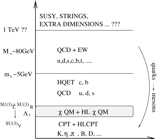
Figure 1: Energy hierarchy in interactions of elementary particles.

The ideas from the chiral quark model of the pure light sector chiqm ; pider ; epb ; BEF has been extended to the sector involving a heavy quark ($c$ or $b$) and thereby to heavy-light mesons HLchiqm . Such models we name heavy-light chiral quark models (HL$\chi$QM). Also in this case, one may integrate out the light and heavy quarks and obtain chiral Lagrangians involving light and heavy mesons wisitchpt . That is, we calculate the parameters of chiral Lagrangian terms, where the description of heavy mesons are in accordance with heavy quark effective field theory (HQEFT) neu . In our approach AHJOE we extended the formalism of HLchiqm to include gluon (vacuum) condensates.

One important motivation for the inclusion of gluon condensates is the possibillity to estimate non-factorizable (colour suppressed) contributions in non-leptonic decays. For instance, $K-\bar{K}$-mixing and the $\Delta I=1/2$ rule for $K\rightarrow 2\pi$ can be understood in a reasonable way within the $\chi$QM pider ; BEF including gluon condensates. Especially, the suppression of the $I=2$ amplitude found for $K\rightarrow 2\pi$ is also in agreement with generalized factorization cheng . Furthermore, it allows us for instance to consider decays where the gluonic aspect of $\eta^{\prime}$ is relevant EHP , and some aspects of $D$-meson decays EFZ . The most important application is to calculate non-factorizable contributions to $B-\bar{B}$-mixing ahjoeB , where our approach includes $1/m_{b}$ corrections and chiral corrections both from loops and counterterms. Also processes of the type $B\rightarrow D\bar{D}$ are calculable EFH . It should be emphasized that the HL$\chi$QM can not, -in its present form, be used for heavy to light transitions like $B\rightarrow\pi K$, where QCD factorization BBNS or soft collinear theory(SCET) SCET is often applied . Still, in the last section, we suggest how an extension to this case might be performed. We also suggest how the $\chi$QM might be extended to include light vectors ($\rho,\omega,K^{*}$).

II Chiral perturbation theory

II.1 The pure light sector

Quarks are the fundamental hadronic matter. However, the particles we observe are those built out of them: baryons and mesons. In the sector of the lowest mass pseudoscalar mesons (the would-be Goldstone bosons: $\pi$, $K$ and $\eta$) the interactions can be described in terms of an effective theory, the chiral Lagrangian, that includes only these states. The chiral Lagrangian and chiral perturbation theory ($\chi$PT) Weinb ; GassL provide a faithful representation of this sector of the Standard Model after the quark and gluon degrees of freedom have been integrated out. The form of this effective field theory and all its possible terms are determined by $SU_{L}(3)\times SU_{R}(3)$ chiral invariance and Lorentz invariance. Terms which explicitly break chiral invariance are introduced in terms of the quark mass matrix ${\cal M}_{q}$.

The strong chiral lagrangian is completely fixed to the leading order in momenta by symmetry requirements and the Goldstone boson’s decay amplitudes:

$${\cal L}_{\rm strong}^{(2)}=\frac{f^{2}}{4}Tr\left(D_{\mu}\Sigma D^{\mu}\Sigma^{{\dagger}}\right)+\frac{f^{2}}{2}B_{0}Tr\left({\cal M}_{q}\Sigma^{{\dagger}}+\Sigma{\cal M}_{q}^{{\dagger}}\right)\,,$$ (1)

where the covariant derivative $D^{\mu}$ contains the photon field, and ${\cal M}_{q}=\mbox{diag}[m_{u},m_{d},m_{s}]$. The quantity $B_{0}$ is defined by $\langle\bar{q}_{i}q_{j}\rangle=-f^{2}B_{0}\delta_{ij}$, where

$$(m_{s}+m_{d})\langle\bar{q}q\rangle=-f_{K}^{2}m_{K}^{2}\;,\quad(m_{u}+m_{d})\langle\bar{q}q\rangle=-f_{\pi}^{2}m_{\pi}^{2}\;,$$ (2)

in the PCAC limit. The quantity $\langle\bar{q}q\rangle$ is the quark condensate, being of order (-240 MeV$)^{3}$. The $SU_{L}(3)\times SU_{R}(3)$ field $\Sigma$ contains the pseudoscalar octet $\Pi$:

$$\Sigma\equiv\exp\left(\frac{2i}{f}\,\Pi\right)\;\,,\quad\Pi=\frac{\lambda^{a}}{2}\phi^{a}(x)=\frac{1}{\sqrt{2}}\left[\begin{array}[]{ccc}\frac{\pi^{0}}{\sqrt{2}}+\frac{\eta_{8}}{\sqrt{6}}&\pi^{+}&K^{+}\\ \pi^{-}&-\frac{\pi^{0}}{\sqrt{2}}+\frac{\eta_{8}}{\sqrt{6}}&K^{0}\\ K^{-}&\overline{K^{0}}&-\frac{2}{\sqrt{6}}\eta_{8}\end{array}\right]\;.$$ (6)

The quantity $f$ is, to lowest order, identified with the pion decay constant $f_{\pi}$ (and equal to $f_{K}$ before chiral loops are introduced).

When the matrix $\Sigma$ is expanded in powers of $f^{-1}$, the zeroth order term obtained from (1) is the free Klein-Gordon Lagrangian for the pseudoscalar particles. From this Lagrangian one might deduce the (left-handed) current

$$J^{n}_{\mu}=-i\frac{f^{2}}{2}Tr\left[\lambda^{n}\Sigma D^{\mu}\Sigma^{{\dagger}}\right]\;,$$ (7)

where $n$ is a flavour octet index and $\lambda_{n}$ a $SU(3)$ flavour matrix.

For the next-to-leading order Lagrangian ${\cal L}_{\rm strong}^{(4)}$ there are ten terms and thereby ten coefficients $L_{i}$ to be determined GassL either experimentally or by means of some model. Some of these play an important role in the physics of $\epsilon^{\prime}$ in $K\rightarrow 2\pi$ decaysepsK . As examples, we display the $L_{5}$ and $L_{8}$ terms in governing much of the penguin physics:

$$L_{5}\,B_{0}\,Tr\left[D_{\mu}\Sigma^{{\dagger}}D^{\mu}\Sigma\left({\cal M}_{q}^{{\dagger}}\Sigma+\Sigma^{{\dagger}}{\cal M}_{q}\right)\right]\;,$$ (8)

and

$$L_{8}\,B_{0}\,Tr\left[{\cal M}_{q}^{{\dagger}}\Sigma{\cal M}_{q}^{{\dagger}}\Sigma+{\cal M}_{q}\Sigma^{{\dagger}}{\cal M}_{q}\Sigma^{{\dagger}}\right]\,.$$ (9)

Under the action of the elements $V_{R}$ and $V_{L}$ of the chiral group $SU_{R}(3)\times SU_{L}(3)$, the field $\Sigma$ transforms as:

$$\Sigma\rightarrow V_{L}\Sigma V_{R}^{{\dagger}}\;,$$ (10)

and accordingly for the conjugated fields. Formally, ${\cal M}_{q}$ is given the same transformation properties as $\Sigma$, and ${\cal M}_{q}^{\dagger}$ as $\Sigma^{\dagger}$.

II.2 The heavy light sector

The strong chiral Lagrangian for the heavy light sector is wisitchpt ; HLchpt :

$${\cal L}_{Str}\, =\,\mp Tr\left[\overline{H^{(\pm)}_{vk}}(iv\cdot{\cal D}_{hk})H^{(\pm)}_{vh}\right]\,-\,g_{\cal A}Tr\left[\overline{H^{(\pm)}_{vk}}H^{(\pm)}_{vh}\gamma_{\mu}\gamma_{5}{\cal A}^{\mu}_{hk}\right]$$ (11)

$$+2\lambda_{1}Tr\left[\overline{H^{(\pm)}_{vk}}H^{(\pm)}_{vh}(\widetilde{M}_{q}^{V})_{hk}\right]+\frac{e\beta}{4}Tr[\overline{H^{(\pm)}_{vk}}H^{(\pm)}_{vh}\sigma\cdot F\,(Q_{q}^{\xi})_{hk}]\,+......$$

where $k,h$ are $SU(3)$ triplet indices, and $v$ is the velocity of the heavy meson. The ellipses indicate other terms (of higher order, say), and $i{\cal D}_{hk}^{\mu}=\delta_{hk}D^{\mu}+{\cal V}^{\mu}_{hk}$. Moreover, $Q^{\xi}_{q}=(\xi^{\dagger}Q_{q}\xi+\xi Q_{q}\xi^{\dagger})/2$, where $Q_{q}$ is the $SU(3)$ charge matrix for light quarks, $Q_{q}=diag(2/3,-1/3,-1/3)$, and $F$ is the electromagnetic field tensor. $H_{vk}^{(\pm)}$ is the heavy meson field containing a spin zero and spin one boson:

$$H_{vk}^{(\pm)} {\equiv}P_{\pm}(v)(P_{k}^{(\pm)\mu}\gamma_{\mu}-iP_{k}^{(\pm)5}\gamma_{5})\;,$$ (12)

$$\overline{H_{vk}^{(\pm)}} =\gamma^{0}(H_{vk}^{(\pm)})^{\dagger}\gamma^{0}=\left[(P_{k}^{(\pm)\mu})^{\dagger}\gamma_{\mu}-i(P_{k}^{(\pm)5})^{\dagger}\gamma_{5}\right]P_{\pm}\;,$$

where

$$P_{\pm}(v)=(1\pm\gamma\cdot v)/2$$ (13)

are projection operators. The fields $P^{(\pm)5}(P^{(\pm)\mu})$ represent heavy-light mesons, $0^{-}(1^{-})$, with velocity $v$. The signs $\pm$ refers to particles and anti-particles respectively, and will sometimes be omitted in the following when unnecessary.

The vector and axial vector fields ${\cal V}_{\mu}$ and ${\cal A}_{\mu}$ are given by:

$${\cal V}_{\mu}{\equiv}\frac{i}{2}(\xi^{\dagger}\partial_{\mu}\xi+\xi\partial_{\mu}\xi^{\dagger})\qquad;\qquad{\cal A}_{\mu}{\equiv}-\frac{i}{2}(\xi^{\dagger}\partial_{\mu}\xi-\xi\partial_{\mu}\xi^{\dagger})\;.$$ (14)

The fields $\xi$ and $H_{v}$ transform as

$$\xi\rightarrow U\,\xi\,V_{R}^{\dagger}\,=V_{L}\xi U^{\dagger}\quad,\qquad H_{v}\rightarrow H_{v}\,U^{\dagger}\;,$$ (15)

where $U\,\epsilon\;SU(3)_{V}$, the unbroken symmetry.

The vector and axial fields transform as

$${\cal V}_{\mu}\rightarrow U\,{\cal V}_{\mu}\,U^{\dagger}\;+\;iU\partial_{\mu}\,U^{\dagger}\quad,\qquad{\cal A}_{\mu}\rightarrow U{\cal A}_{\mu}\,U^{\dagger}\;.$$ (16)

The vector field ${\cal{V}}^{\mu}$ is seen to transform as a gauge field under local $SU(3)_{V}$, and can only appear in combination with a derivative as a covariant derivative $(i\partial^{\mu}+{\cal{V}}^{\mu})$. The quantity $\widetilde{M_{q}}^{V}$ (as well as the orthogonal combination $\widetilde{M_{q}}^{A}$) is related to the current mass term:

$$\widetilde{M}_{q}^{V}\,{\equiv}\,\frac{1}{2}(\xi^{\dagger}{\cal M}_{q}\xi^{\dagger}\,+\xi{\cal M}_{q}^{{\dagger}}\xi)\quad;\qquad\widetilde{M}_{q}^{A}{\equiv}-\frac{1}{2}(\xi^{\dagger}{\cal M}_{q}\xi^{\dagger}-\xi{\cal M}_{q}^{{\dagger}}\xi)\;.$$ (17)

The heavy-light weak current, to zeroth order in $1/m_{Q}$ and chiral counting, is represented by:

$$J_{k}^{\alpha}(0)=\frac{\alpha_{H}}{2}Tr\left[\xi^{\dagger}_{hk}\Gamma^{\alpha}H_{vh}\right]\;,$$ (18)

and under $SU(3)_{L}$ it transforms as

$$J_{k}^{\alpha}\rightarrow J_{h}^{\alpha}\left(V_{L}^{\dagger}\right)_{hk}\;.$$ (19)

This current has also (counter) terms, of higher order in the chiral counting, needed to make the chiral loops finite:

$$J^{\mu}_{k}({\cal M})=\frac{\omega_{1}}{2}Tr[\xi^{\dagger}_{hk}\,\Gamma^{\mu}{H_{v}}_{l}\,\widetilde{{\cal M}^{V}_{lh}}]+\frac{\omega_{1}^{\prime}}{2}Tr[\xi^{\dagger}_{kh}\,\Gamma^{\mu}{H_{v}}_{h}]\,\widetilde{{\cal M}^{V}_{ll}}\;,$$ (20)

where the parameters $\omega_{1}$ and $\omega_{1}^{\prime}$ are commented on in section IV-C. To leading order, $\Gamma^{\alpha}=\gamma^{\alpha}L$, where $L$ is the left - handed projector in Dirac space, $L=(1-\gamma_{5})/2$. However, this is slightly modified by perturbative QCD for $\mu$ below $m_{Q}$, which gives neu

$$\Gamma^{\alpha}\,{\equiv}\,C_{\gamma}(\mu)\,\gamma^{\alpha}\,L\,+\,C_{v}(\mu)\,v^{\alpha}\,R\;,$$ (21)

where $R$ is the right - handed projector, $R=(1+\gamma_{5})/2$ . The coefficients $C_{\gamma,v}(\mu)$ are determined by QCD renormalization for $\mu<m_{Q}$. They have been calculated to NLO and the result is the same in $MS$ and $\overline{MS}$ schemeCgamma . ($C_{\gamma}$ is close to one and $C_{v}$ is rather small). Corrections to the weak current of order $1/m_{Q}$ will be discussed in section V.

Before closing this section, we write down the bosonized $b\rightarrow c$ transition current in terms of the heavy fields

$$\overline{Q_{v_{b}}^{(+)}}\,\gamma^{\mu}LQ_{v_{c}}^{(+)}\;\longrightarrow\;-\zeta(\omega)Tr\left[\overline{H_{c}^{(+)}}\gamma^{\alpha}LH_{b}^{(+)}\right],$$ (22)

where $\zeta(\omega)$ is the Isgur-Wise function for the $\bar{B}\rightarrow D$ transition isgur . The indices on the heavy fields here refer to the the $b$- and $c$-quarks with velocities $v_{b}$ and $v_{c}$, with $\omega\equiv v_{b}\cdot v_{c}$. The current for $D\overline{D}$ production is :

$$\overline{Q_{v_{c}}^{(+)}}\,\gamma^{\mu}\,LQ_{\bar{v}}^{(-)}\;\longrightarrow\;-\zeta(-\lambda)Tr\left[\overline{H_{c}^{(+)}}\gamma^{\alpha}LH_{\bar{c}}^{(-)}\right]\;,$$ (23)

where the Isgur-Wise function $\zeta(-\lambda)$ is (in general) complex. We have $\lambda=v_{c}\cdot\bar{v}\,$, where $\bar{v}$ is the velocity of $\bar{c}$.

III The chiral quark model ($\chi$QM)

III.1 The Lagrangians for $\chi$QM

The light quark sector is described by the chiral quark model ($\chi$QM), having a standard QCD term and a term describing interactions between quarks and (Goldstone) mesons bijnes ; chiqm ; epb ; pider ; BEF :

$${\cal L}_{\chi QM}=\bar{q}_{L}i\gamma\cdot D\,q_{L}\,+\,\bar{q}_{R}i\gamma\cdot D\,q_{R}-\bar{q}_{L}{\cal M}_{q}\,q_{R}\,-\bar{q}_{R}{\cal M}_{q}^{\dagger}\,q_{L}-m(\bar{q}_{R}\Sigma^{\dagger}q_{L}+\bar{q}_{L}\Sigma q_{R})\;,$$ (24)

where $m$ is the ($SU(3)$ - invariant) constituent quark mass for light quarks $q^{T}=(u,d,s)$. The left- and right-handed projections $q_{L}$ and $q_{R}$ are transforming after $SU(3)_{L}$ and $SU(3)_{R}$ respectively:

$$q_{L}\rightarrow V_{L}\,q_{L}\qquad\mbox{and}\qquad q_{R}\rightarrow V_{R}\,q_{R}\;.$$ (25)

From (24) we deduce the Feynman rules. For instance, the $Pq\bar{q}$ coupling is $(m\gamma_{5}/f)$ times some $SU(3)$ factor ($P$ is a pseudoscalar meson $\pi,K,\eta$). From such Feynman rules, and including the quark propagator $S(p)=(\gamma\cdot p-M_{q})^{-1}$, we can calculate aplitudes for, say, $\pi-\pi$ scattering in the strong sector. Here $M_{q}=m+m_{q}$ is the total mass. Alternatively one might keep only the constituent mass $m$ in the propagator, and take the current mass $m_{q}$ as a coupling. Incuding also the Feynman rules for weak vertices, one might calculate BEF ; epb amplitudes for non-leptonic decays in terms of quark loops representing $f_{\pi}$ and the semileptonic form factors $f_{\pm}$, but also for more complicated cases.

Also, as a more exotic example, one may calculate the effect of the electroweak $s\rightarrow d$ self-energy transition contribution to $K\rightarrow 2\pi$ as shown in Fig. 2. This is an off-shell effect which vanish in the free quark case, but is non-zero for bound quarks and proportional to $m$ within our framework epb .

Figure 2: Contribution to the process $K\rightarrow 2\pi$ from the non-diagonal $s\rightarrow d$ transition.

Chiral Lagrangians, either in the pure strong sector or for non-leptonic decays, are however easier to obtain in a more transparent way within the “rotated version” of the $\chi$QM with flavour rotated quark fields $\chi$ given by:

$$\chi_{L}=\xi^{\dagger}q_{L}\quad;\qquad\chi_{R}=\xi q_{R}\quad;\qquad\xi\cdot\xi=\Sigma\;.$$ (26)

The constituent quark fields $\chi_{L}$ and $\chi_{R}$ transform in a simple way under $SU(3)_{V}$:

$$\chi_{L}\rightarrow U\,\chi_{L}\quad,\qquad\chi_{R}\rightarrow U\;\chi_{R}\;.$$ (27)

In the rotated version, the chiral interactions are rotated into the kinetic term while the interaction term proportional to $m$ in (24) become a pure (constituent) mass term chiqm ; BEF :

$${\cal L}_{\chi QM}=\overline{\chi}\left[\gamma^{\mu}(iD_{\mu}+{\cal V}_{\mu}+\gamma_{5}{\cal A}_{\mu})-m\right]\chi-\overline{\chi}\widetilde{M_{q}}\chi\;,$$ (28)

which is manifestly invariant under $SU(3)_{V}$. Moreover,

$$\widetilde{M_{q}}{\equiv}\widetilde{M}_{q}^{V}+\widetilde{M}_{q}^{A}\gamma_{5}\;,$$ (29)

where $\widetilde{M}_{q}^{V,A}$ are given in (17).

In the light sector, the various pieces of the strong Lagrangian in section II-A can now be obtained by integrating out the constituent quark fields $\chi$, and these pieces can be written in terms of the fields ${\cal A}_{\mu}\,,\,\widetilde{M}_{q}^{V}$ and $\widetilde{M}_{q}^{A}$ This can easily be seen by using the relation

$${\cal{A}}_{\mu}\;=\;-\frac{1}{2i}\xi\,(D_{\mu}\Sigma^{\dagger})\,\xi\;=+\;\frac{1}{2i}\xi^{\dagger}\,(D_{\mu}\Sigma)\,\xi^{\dagger}\;.$$ (30)

In our model, the hard gluons are integrated out and we are left with soft gluonic degrees of freedom. These gluons can be described using the external field technique, and their effect will be parameterized by vacuum expectation values, i.e. the gluon condensate ${\langle}\frac{\alpha_{s}}{\pi}G^{2}{\rangle}$. Gluon condensates with higher dimension could also be included, but we truncate the expansion by keeping only the condensate with lowest dimension.

When calculating the soft gluon effects in terms of the gluon condensate, we follow the prescription given in nov .

Figure 3: Feynmanrule for the light quark -soft gluon vertex.

The calculation is easily carried out in the Fock - Schwinger gauge. In this gauge one can expand the gluon field as :

$$A_{\mu}^{a}(k)=-\frac{i(2\pi)^{4}}{2}G^{a}_{\rho\mu}(0)\frac{\partial}{\partial k_{\rho}}\delta^{(4)}(k)+\cdots\,.$$ (31)

In some simple cases one may also use the light quark propagator in a gluonic background (to first order in the gluon field):

$$S_{1}(p,G)=-\frac{g_{s}}{4}G^{b}_{\alpha\beta}t^{b}\left[\sigma^{\alpha\beta}(\gamma\cdot p+m)\,+\,(\gamma\cdot p+m)\sigma^{\alpha\beta}\right](p^{2}-m^{2})^{-2}\;,$$ (32)

where $g_{s}$ is the strong coupling constant, $a$ and $b$ are colour octet indices, and $t^{a}$ are the colour matrices. In general one should stick to the prescription in nov in order to get correct results. Since each vertex in a Feynman diagram is accomplished with an integration we get the Feynman rule given in Fig. 3. The gluon condensate contributions are obtained by the replacement

$$g_{s}^{2}G_{\mu\nu}^{a}G_{\alpha\beta}^{b}\;\rightarrow\frac{4\pi^{2}}{(N_{c}^{2}-1)}\delta^{ab}{\langle}\frac{\alpha_{s}}{\pi}G^{2}{\rangle}\frac{1}{12}(g_{\mu\alpha}g_{\nu\beta}-g_{\mu\beta}g_{\nu\alpha})\,.$$ (33)

.

III.2 Bosonization of the $\chi$QM

The Lagrangians (24) or (28) from the previous section can now be used for bosonization, i.e. to integrate out the quark fields. This can be done in the path integral formalism, or as we do here, by expanding in terms of Feynman diagrams. Within the $\chi$QM, with Feynman rules obtained from (24) one may calculate the simple quark loop amplitude for $\pi\rightarrow W$ which defines $f$ (the bare $f_{\pi}$) in terms of a logarithmicly divergent integral $I_{2}$ times the coupling $\sim m/f$. Including also the gluon condensate contribution one obtains pider ; epb ; BEF :

$$f^{2}=-i4m^{2}N_{c}I_{2}+\frac{1}{24m^{2}}{\langle}\frac{\alpha_{s}}{\pi}G^{2}{\rangle}\;,$$ (34)

where $I_{2}$ is the following logarithmic divergent integral ($d$ is the dimension of space within dimensional regularization):

$$I_{2}\, {\equiv}\, \int\frac{d^{d}k}{(2\pi)^{d}}\frac{1}{(k^{2}-m^{2})^{2}}\,.$$ (35)

Equivalently, one may obtain the (kinetic part of the) strong Lagrangian in (1) by attaching two axial fields ${\cal A}_{\mu}$ to a vacuum polarization like quark loop diagram by using (28). Then one obtains:

$$i{\cal{L}}^{(2)}_{str}\,=-N_{c}\,\int\frac{d^{d}p}{(2\pi)^{d}}\,Tr\,\left[\left(\gamma_{\sigma}\gamma_{5}{\cal{A}}^{\sigma}\right)\,S(p)\,\left(\gamma_{\rho}\gamma_{5}{\cal{A}}^{\rho}\right)\,S(p)\right]\,=\,f^{2}Tr\,\left[{\cal{A}}_{\mu}{\cal{A}}^{\mu}\right]\;,$$ (36)

where the trace is both in flavor and Dirac spaces (a similar diagram with glouns should also be added). This is easily seen by using the relation (30), provided $f^{2}$ is given by (34). The eq. (36) give the Lagrangian (1) in the light sector by applying (30).

The quark condensate is:

$${\langle}\,\overline{q}q\,{\rangle}=-iN_{c}Tr\int\frac{d^{d}p}{(2\pi)^{d}}S(p)\,=\,-4imN_{c}I_{1}-\frac{1}{12m}{\langle}\frac{\alpha_{s}}{\pi}G^{2}{\rangle}\;,$$ (37)

where $I_{1}$ is the quadratically divergent integral

$$I_{1}\, {\equiv} \,\int\frac{d^{d}k}{(2\pi)^{d}}\frac{1}{k^{2}-m^{2}}\;.$$ (38)

Here the propagator $S$ has to be understood at the one in the gluon field up to second order and the a priori divergent integrals $I_{1,2}$ have to be interpreted as the regularized ones. The physical values of $I_{1,2}$ are determined by the physical values of $f$ and ${\langle}\,\overline{q}q\,{\rangle}$. In general, by coupling the fields ${\cal{A}}_{\mu}$ and $\widetilde{M}_{q}^{V,A}$ to quark loops, the chiral Lagrangian terms and their coefficients within the light sector can be obtained.

Similarly, we may bosonize the weak currents. The left handed current can be written

$$\bar{q}_{L}\gamma^{\mu}\lambda^{n}q_{L}\,=\,\,\bar{\chi}_{L}\gamma^{\mu}\Lambda^{n}\,\chi_{L}\;;\qquad\Lambda^{n}\,\equiv\,\xi^{\dagger}\lambda^{n}\,\xi\;.$$ (39)

The lowest order term ${\cal O}(p)$ is obtained when the vertex $\Lambda^{n}$ from (39) and axial vertex ($\sim{\cal A}_{\mu}$) from (28) are entering a quark loop (see Fig. 4):

$$j^{n}_{\mu}({\cal{A}})\,=-\,iN_{c}\int\frac{d^{d}p}{(2\pi)^{d}}\,Tr\,\left[\left(\gamma_{\mu}L\,\Lambda^{n}\right)S(p)\,\left(\gamma_{\sigma}\gamma_{5}{\cal{A}}^{\sigma}\right)\,S(p)\,\right]\;\sim\;Tr\,\left[\Lambda^{n}\,{\cal{A}}_{\mu}\right]\;,$$ (40)

which coincides with (7) when (30) is used.

Figure 4: Feynman diagram for bosonization of the left-handed current to order ${\cal O}(p)$.

As a more non-trivial example, to obtain a non-zero non-factorizable contribution to $D^{0}\rightarrow K^{0}\bar{K^{0}}$ at tree level, one has to consider the coloured current $j^{n,a}_{\mu}$ to ${\cal O}(p^{3})$, involving insertions of the “mass fields” $\widetilde{M}_{q}$ in (29) EFZ . (This coloured current is obtained by Fierz transformations of the relevant four quark operator). From Fig. 5, one obtains the contribution:

Figure 5: Diagram for bosonization of the colour current to ${\cal O}(p^{3})$.

$$j^{n,a}_{\mu}({\mbox{Fig. 5}})\,=i\,\int\frac{d^{d}p}{(2\pi)^{d}}\,Tr\,\left[\left(\gamma_{\mu}L\,\Lambda^{n}t^{a}\right)\,S(p)\,\left(\gamma_{\sigma}\gamma_{5}{\cal{A}}^{\sigma}\right)\,S(p)\,\widetilde{{M}_{q}}\,S_{1}(p,G)\right]\,,$$ (41)

Summing all six diagrams with permutated vertices compared to the one in Fig. 5 we obtain in total :

$$j^{n,a}_{\mu}(G,\xi,{\cal{A}},\widetilde{{\cal{M}}_{q}})\,=\,\frac{g_{s}}{12m}\frac{1}{16\pi^{2}}\,G^{a,\kappa\lambda}\left[i\varepsilon_{\mu\rho\kappa\lambda}\;T_{\varepsilon}^{n,\rho}\,+\,\left(g_{\mu\kappa}g_{\rho\lambda}\;-\;g_{\mu\lambda}g_{\rho\kappa}\right)T_{g}^{n,\rho}\right]\;,$$ (42)

where (we have used the analytical computer program FORM FORM )

$$T_{\varepsilon}^{n,\rho}\,=\,4\,S^{K}_{\rho}\,-3(S^{L}_{\rho}+S^{R}_{\rho})\;,\;\;T_{g}^{n,\rho}\,=S^{L}_{\rho}\,-\,S^{R}_{\rho}\;.$$ (43)

The $S^{\prime}s$ are chiral Lagrangian terms:

$$\begin{split}S^{L}_{\rho}\,&\equiv\,Tr\left[\Lambda^{n}{\cal{A}}_{\rho}\,\widetilde{M}_{q}^{L}\right]\,=\,\frac{1}{2i}Tr\left[\lambda^{n}(D_{\rho}\Sigma)\,{\cal{M}}_{q}^{\dagger}\right]\;,\\ S^{R}_{\rho}\,&\equiv\,Tr\left[\Lambda^{n}\,\widetilde{M}_{q}^{R}\,{\cal{A}}^{\rho}\,\right]\,=\,\frac{-1}{2i}Tr\left[\lambda^{n}\,{\cal{M}}_{q}\,(D_{\rho}\Sigma^{\dagger})\,\right]\;,\\ S^{K}_{\rho}\,&\equiv\,\frac{1}{2}Tr\left[\Lambda^{n}\left({\cal{A}}^{\rho}\,\widetilde{M}_{q}^{R}\,+\,\widetilde{M}_{q}^{L}\,{\cal{A}}^{\rho}\right)\,\right]\\ &=\,\frac{1}{4i}Tr\left[\lambda^{n}\left((D_{\rho}\Sigma)\,\Sigma^{\dagger}{\cal{M}}_{q}\Sigma^{\dagger}\,-\,\Sigma{\cal{M}}_{q}^{\dagger}\Sigma(D_{\rho}\Sigma^{\dagger})\right)\right]\;.\end{split}$$ (44)

The current (42) has to be be combined with the left-handed colour current for $D$-meson decay later given in (93) to obtain a contribution to $D^{0}\rightarrow K^{0}\bar{K^{0}}$ EFZ .

IV The Heavy - Light Chiral Quark Model (HL$\chi$QM)

IV.1 The Lagrangian for HL$\chi$QM

Our starting point is the following Lagrangian containing both quark and meson fields:

$${\cal L}={\cal L}_{HQEFT}+{\cal L}_{\chi QM}+{\cal L}_{Int}\;,$$ (45)

where neu

$${\cal L}_{HQEFT}=\,\pm\,\overline{Q_{v}^{(\pm)}}\,iv\cdot D\,Q_{v}^{(\pm)}+\frac{1}{2m_{Q}}\overline{Q_{v}^{(\pm)}}\,\left(-C_{M}\frac{g_{s}}{2}\sigma\cdot G\,+\,(iD_{\perp})_{\text{eff}}^{2}\right)\,Q_{v}^{(\pm)}+{\cal O}(m_{Q}^{-2})$$ (46)

is the Lagrangian for heavy quark effective field theory (HQEFT). The heavy quark field $Q_{v}^{(+)}$ annihilates a heavy quark with velocity $v$ and mass $m_{Q}$. Similarly, $Q_{v}^{(-)}$ annihilates a heavy anti-quark. Moreover, $D_{\mu}$ is the covariant derivative containing the gluon field (eventually also the photon field), and $\sigma\cdot G=\sigma^{\mu\nu}G^{a}_{\mu\nu}t^{a}$, where $\sigma^{\mu\nu}=i[\gamma^{\mu},\gamma^{\nu}]/2$, and $G^{a}_{\mu\nu}$ is the gluonic field tensor. This chromo-magnetic term has a factor $C_{M}$, being one at tree level, but slightly modified by perturbative QCD.(When the covariant derivative also contains the photon field, there is also a corresponding magnetic term $\sim\sigma\cdot F$, where $F^{\mu\nu}$ is the electromagnetic tensor). Furthermore, $(iD_{\perp})_{\text{eff}}^{2}=C_{D}(iD)^{2}-C_{K}(iv\cdot D)^{2}$. At tree level, $C_{D}=C_{K}=1$. Here, $C_{D}$ is not modified by perturbative QCD, while $C_{K}$ is different from one due to perturbative QCD corrections for $\mu<m_{Q}$ GriFa . We observe that soft gluons coupling to a heavy quark is suppressed by $1/m_{Q}$, since to leading order the vertex is proportional to $v_{\mu}v_{\nu}G^{a\mu\nu}=0$, $v_{\mu}$ being the heavy quark velocity.

In the heavy - light case, the generalization of the meson - quark interactions in the pure light sector $\chi$QM is given by the following $SU(3)$ invariant Lagrangian:

$${\cal L}_{Int}=-G_{H}\,\left[\overline{\chi}_{k}\,\overline{H_{vk}^{(\pm)}}\,Q_{v}^{(\pm)}\,+\overline{Q_{v}^{(\pm)}}\,H_{vk}^{(\pm)}\,\chi_{k}\right]\,,$$ (47)

where $k$ is a triplet $SU(3)$- index and $G_{H}$ is a coupling constant. Note that in HLchiqm , $G_{H}=1$ is used. However, in that case one used a renormalization factor for the heavy meson fields $H_{v}$, which is equivalent. The interaction Lagrangian (47) can, as for the $\chi$QM, be obtained from a NJL model. This has been done in HLchiqm (-as for the light sector bijnes ).

IV.2 Bosonization within the HL$\chi$QM

The interaction term ${\cal{L}}_{Int}$ in (47) can now be used to bosonize the model, i.e. integrate out the quark fields. This can be done in terms of Feynman diagrams as we do here, by attaching the external fields $H_{v}^{a},\overline{H_{v}^{a}},{\cal{V}}^{\mu},{\cal{A}}^{\mu}$ and $\widetilde{M}_{q}^{V,A}$ of section II-B to quark loops, and using (28) and (47). In this way one obtains the strong chiral Lagrangian (11) and terms of higher order in the heavy light sector . Some of the loop integrals will be divergent and have to be related to physical parameters, as for the pure light sector chiqm ; pider ; epb ; BEF . As the pure light sector is a part of our model, we have to keep the relations in (34) and (37) from the pure light sector within the heavy light case studied here. The $1/m_{Q}$ terms will not be discussed in this section, but will be considered later in section V.

From the diagrams in Fig. 6 we obtain the identification for the kinetic term , which by Ward identities is the same as for the term with the vector field ${\cal V}_{\mu}$ attached to the light quark:

$$-iG_{H}^{2}N_{c}\,(I_{3/2}+2mI_{2}+i\frac{(8-3\pi)}{384N_{c}m^{3}}{\langle}\frac{\alpha_{s}}{\pi}G^{2}{\rangle})=1\;,$$ (48)

where $I_{2}$ is given in (35) and

$$I_{3/2}\, {\equiv} \,\int\frac{d^{d}k}{(2\pi)^{d}}\frac{1}{(v\cdot k)(k^{2}-m^{2})}\;,$$ (49)

which formally depends on $v^{2}$ which is equal to one. From the same diagram, with the axial field ${\cal A}_{\mu}$ attached, we obtain the following identification for the axial vector coupling $g_{\cal A}$ :

Figure 6: Bosonization in the strong sector to obtain eq. (11).

$$g_{\cal A}{\equiv}iG_{H}^{2}N_{c}\left(\frac{1}{3}I_{3/2}-2mI_{2}-i\frac{m}{12\pi}-i\frac{(8-3\pi)}{384N_{c}m^{3}}{\langle}\frac{\alpha_{s}}{\pi}G^{2}{\rangle}\right)\;,$$ (50)

As $I_{1}$ and $I_{2}$ are related to the quark condensate and $f_{\pi}$ respectively, the (formally) linearly divergent integral $I_{3/2}$ is related to $\delta g_{\cal A}\equiv 1-g_{\cal A}$, which is found by eliminating $I_{2}$ from eqs. (48) and (50) :

$$\delta g_{\cal A}=-\frac{4}{3}iG_{H}^{2}N_{c}\,\left(I_{3/2}-i\frac{m}{16\pi}\right)\;.$$ (51)

Note that the gluon condensate drops out here. Within a primitive cut-off regularization, $I_{3/2}$ is (in the leading approximation) proportional to the cut-off in first power:

$$I_{3/2}=i\frac{\Lambda}{16\pi}\left(1+{\cal O}(\frac{m}{\Lambda})\right)\;\,,$$ (52)

where the cut-off $\Lambda$, is of the same order as the chiral symmetry breaking scale $\Lambda_{\chi}$. In contrast, $I_{3/2}$ is finite and proportional to $m$ in dimensional regularization. Note that the cut-off $\Lambda$ is only used in qualitative considerations here and in subsection IV-D. Anyway, $I_{3/2}$ is determined by the physical value og $g_{{\cal A}}$.

When attaching $\widetilde{M}_{q}^{V}$ like in Fig. 6 instead of vector or axial vector fields one finds for the mass correction term in (11):

$$2\lambda_{1}{\equiv}iG_{H}^{2}N_{c}(I_{3/2}-2mI_{2}-i\frac{m}{8\pi}-\frac{i(3\pi-4)}{192N_{c}m^{3}}{\langle}\frac{\alpha_{s}}{\pi}G^{2}{\rangle})\;.$$ (53)

The electromagnetic $\beta$ term in (11) is obtained by considering diagrams like those in figure 6, but with the vector and axial vector fields ${\cal V}_{\mu}$ or ${\cal A}_{\mu}$ replaced by a photon field tensor:

$$\beta=\frac{G_{H}^{2}}{2}\left\{-4iN_{c}I_{2}+\frac{N_{c}}{4\pi}-\left(\frac{32+3\pi}{576m^{4}}\right){\langle}\frac{\alpha_{s}}{\pi}G^{2}{\rangle}\right\}\,.$$ (54)

Within the full theory (SM) at quark level, the weak current is :

$$J_{k}^{\alpha}={\overline{q_{k}}_{L}}\,\gamma^{\alpha}\,Q$$ (55)

where $Q$ is the heavy quark field in the full theory. Within HQEFT this current will, below the renormalization scale $\mu=m_{Q}\,(=m_{b},m_{c})$, be modified in the following way:

$$J_{k}^{\alpha}={\overline{\chi}}_{h}\xi^{\dagger}_{hk}\Gamma^{\alpha}Q_{v}\,+{\cal O}(m_{Q}^{-1})\;,$$ (56)

The operator in equation (56) can be bosonized by calculating the Feynman diagrams shown in Fig. 7 which gives the bosonized current in (18) with:

$$\alpha_{H}{\equiv}-2iG_{H}N_{c}\left(-I_{1}+mI_{3/2}+\frac{i(3\pi-4)}{384N_{c}m^{2}}{\langle}\frac{\alpha_{s}}{\pi}G^{2}{\rangle}\right)\;.$$ (57)

Figure 7: Diagrams for bosonization of the left handed quark current.

To first order in the chiral expansion we obtain the bosonized current obtained by attaching one extra field ${\cal A_{\nu}}$ to the quark loops in Fig. 7:

$$J_{k}^{\alpha}(1)\,=\,\frac{1}{2}Tr\left[\xi^{\dagger}_{hk}\Gamma^{\alpha}H_{vh}(\alpha_{H\gamma}^{(1)}\gamma^{\nu}\gamma_{5}+\alpha_{Hv}^{(1)}v^{\nu}\gamma_{5}){\cal A_{\nu}}\right]\;,$$ (58)

where the quantities $\alpha_{H}^{(1)}$ are given by expressions similar to (57).

The coupling $\alpha_{H}$ in (18) is related to the physical decay constants $f_{H}$ and $f_{H^{*}},$ in the following way (for $H=B,D$):

$${\langle}0|\overline{u}\gamma^{\alpha}\gamma_{5}b|H{\rangle}=-2\,{\langle}0|J_{a}^{\alpha}|H{\rangle}\,=iM_{H}f_{H}v^{\alpha}\;,$$ (59)

Taking the trace over the gamma matrices in (18), we obtain a relation for $\alpha_{H}$ and the relations between the heavy meson decay constants $f_{H}$ and $f_{H^{*}}$ (for $H=B,D$) :

$$\alpha_{H}=\frac{f_{H}\sqrt{M_{H}}}{C_{\gamma}(\mu)+C_{v}(\mu)}=\frac{f_{H^{*}}\sqrt{M_{H^{*}}}}{C_{\gamma}(\mu)}\;\;,$$ (60)

where the model dictates us to put $\mu=\Lambda_{\chi}$. Later, in section V-B, we will see how chiral corrections and $1/m_{Q}$ corrections modify this relation.

IV.3 Constraining the parameters of the HL$\chi$QM

The gluon condensate can be related to the chromomagnetic interaction :

$$\mu_{G}^{2}(H)=\frac{1}{2M_{H}}C_{\text{M}}(\mu){\langle}H|\bar{Q_{v}}\frac{1}{2}\sigma\cdot GQ_{v}|H{\rangle}\,,$$ (61)

where the coefficient $C_{\text{M}}(\mu)$ contains the short distance effects down to the scale $\mu$ and has been calculated to next to leading order ($NLO$) neub . The chromomagnetic operator is responsible for the splitting between the $1^{-}$ and $0^{-}$ state, and is known from spectroscopy,

$$\mu_{G}^{2}(H)\,=\,\frac{3}{2}m_{Q}(M_{H^{*}}-M_{H})\;.$$ (62)

An explicit calculation of the matrix element in equation (61) gives

$$\mu_{G}^{2}=\eta_{2}\frac{G_{H}^{2}}{m}{\langle}\frac{\alpha_{s}}{\pi}G^{2}{\rangle}\;,\quad\text{where}\quad\,\eta_{2}\,{\equiv}\,\frac{(\pi+2)}{32}C_{M}(\Lambda_{\chi})\,.$$ (63)

Combining the eqs. (34), (37) and (63) we obtain the following relations :

$${\langle}\frac{\alpha_{s}}{\pi}G^{2}{\rangle}=\frac{\mu_{G}^{2}f^{2}}{2\eta_{2}}\,\frac{1}{\rho}\;\,,\qquad G_{H}^{2}=\frac{2m}{f^{2}}\,\rho\;\,,$$ (64)

where the quantity $\rho$ is of order one and given by

$$\rho\,{\equiv}\,\frac{(1+3g_{\cal A})+\frac{\eta_{1}\mu_{G}^{2}}{\eta_{2}m^{2}}}{4(1+\frac{N_{c}m^{2}}{8\pi f^{2}})}\;\,,$$ (65)

where $\eta_{1}{\equiv}\frac{\pi}{32}$. In the limit where only the leading logarithmic integral $I_{2}$ is kept in (48), we obtain:

$$g_{\cal A}\rightarrow\,1\;,\qquad\rho\rightarrow\,1\;,\qquad\beta\rightarrow\frac{1}{m}\qquad G_{H}\;\rightarrow\;G_{H}^{(0)}\,{\equiv}\,\frac{\sqrt{2m}}{f}\;\,,$$ (66)

which for $g_{\cal A}$ and $\beta$ correspond to the non-relativistic values.

From the eqs. (34), (53), and (63), we find

$$2\lambda_{1}=\frac{1}{2}(3g_{\cal A}-1)+\frac{(9\pi-16)\mu_{G}^{2}}{384\eta_{2}m^{2}}\,.$$ (67)

In the limit (66) we obtain $2\lambda_{1}\rightarrow 1$, as expected. The parameter $\lambda_{1}$ is related to the mass difference $M_{H_{s}}-M_{H_{d}}$. To leading order, we obtained the following expression for the $\beta$-term:

$$\beta=\frac{\rho}{m}\left\{1+\frac{N_{c}m^{2}}{4\pi f^{2}}-\left(\frac{56+3\pi}{576f^{2}m^{2}}\right){\langle}\frac{\alpha_{s}}{\pi}G^{2}{\rangle}\right\}\;,$$ (68)

which is rather sensitive to $m$. Choosing $m$ in the range 250-300 MeV we find Beta $\beta=(2.5\pm 0.6)$ GeV^-1 to be compared with $\beta=(2.7\pm 0.20)$ GeV^-1 extracted from experiment.

Using equation (48) and (37) we may write $\alpha_{H}$ as:

$$\alpha_{H}=\frac{G_{H}}{2}\left(-\frac{{\langle}\,\overline{q}q\,{\rangle}}{m}-2f_{\pi}^{2}(1-\frac{1}{\rho})+\frac{(\pi-2)}{16m^{2}}{\langle}\frac{\alpha_{s}}{\pi}G^{2}{\rangle}\right)\;,$$ (69)

Combining (60) with (69), we obtain EFZ in the leading limit (taking into account the logarithmic and quadratic divergent integrals only, and let $C_{\gamma}\rightarrow 1$, $C_{v}\rightarrow 0$ and $g_{\cal A}\rightarrow 1$ as in (66) ) we obtain the “Goldberger-Treiman like” relation:

$$f_{H}\sqrt{M_{H}}\;\rightarrow\,-\frac{{\langle}\,\overline{q}q\,{\rangle}}{f_{\pi}\sqrt{2m}}\;\;,$$ (70)

which gives the scale for $f_{H}$ (It is, however, numerically a factor 2 off for the $B$-meson).

Using the relations (48), (50) and (65) we obtain for $\alpha_{H\gamma}^{(1)}$ and $\alpha_{Hv}^{(1)}$ in (58):

$$\alpha_{H\gamma}^{(1)} =\frac{2g_{\cal A}}{G_{H}}\;,$$ (71)

$$\alpha_{Hv}^{(1)} =\frac{4}{3}G_{H}\left(\frac{f_{\pi}^{2}}{2m}\left(\frac{1}{\rho}-1\right)+\left[\frac{mN_{c}}{8\pi}+\frac{(\pi+8)}{256m^{3}}{\langle}\frac{\alpha_{s}}{\pi}G^{2}{\rangle}\right]\right)\;.$$ (72)

Moreover, for the mass correction to the weak current given in (20) we find that $\omega_{1}=-4\lambda_{1}/G_{H}$, where $\lambda_{1}$ is given in equation (53) or (67). The term $\omega_{1}^{\prime}$ is subleading in $1/N_{c}$.

The Isgur-Wise function $\zeta(\omega)$ in (22) relates all the form factors describing the processes $B(B^{*})\to D(D^{*})$ in the heavy quark limit. This function can be calculated from the diagrams shown in Fig. 8. The result before $1/m_{Q}$ and chiral corrections is:

$$\zeta(\omega)=\frac{2}{1+\omega}\left(1-\rho\right)+\rho\,r(\omega)\,,$$ (73)

Figure 8: Loop diagrams for bosonizing the $b\rightarrow c$ current, $V^{\mu}=\gamma^{\mu}$, $A^{\mu}=\gamma^{\mu}\gamma_{5}$.

where $\rho$ is given in (65) and $r(\omega)$ is the same function appearing in loop calculations of the anomalous dimension in HQEFT :

$$r(\omega)=\frac{1}{\sqrt{\omega^{2}-1}}\,\text{ln}\left(\omega+\sqrt{\omega^{2}-1}\right)\;.$$ (74)

Note that $\zeta(1)=1$ as it should.

IV.4 The formal limit $m\rightarrow 0$

In this subsection we will discuss the limit of restauration of chiral symmetry, i.e. the limit $m\rightarrow 0$ Beta . In order to do this, we have to consider the various constraints obtained when constructing the HL$\chi$QM AHJOE .

Looking at the equations (34) and (37), one may worry that ${\langle}\,\overline{q}q\,{\rangle}$ and $f$ behaves like $1/m$ in the limit $m\rightarrow 0$ unless one assumes that ${\langle}\frac{\alpha_{s}}{\pi}G^{2}{\rangle}$ also go to zero in this limit. We should stress that the exact limit $m=0$ cannot be taken because our loop integrals will then be meaningless. Still we may let $m$ approach zero without going to this exact limit. In the pure light sector (at least when vector mesons are not included) there are no restrictions on how ${\langle}\frac{\alpha_{s}}{\pi}G^{2}{\rangle}$ might go to zero. In the heavy light sector we have in addition to (34) and (37) also the relations (48) and (50), which put restrictions on the behavior of the gluon condensate ${\langle}\frac{\alpha_{s}}{\pi}G^{2}{\rangle}$ for small masses. As ${\langle}\frac{\alpha_{s}}{\pi}G^{2}{\rangle}$ has dimension mass to the fourth power, we find that ${\langle}\,\overline{q}q\,{\rangle}$ and $f^{2}$ may go to zero if ${\langle}\frac{\alpha_{s}}{\pi}G^{2}{\rangle}$ goes to zero as $m^{4}$ or $m^{3}\Lambda$ (eventually combined with $\ln(m/\Lambda)$). However, the behavior $m^{3}\Lambda$ is inconsistent with the additional equations (64) and (65). Still, from all equations (48), (64), (65), we find the possible solution

$${\langle}\frac{\alpha_{s}}{\pi}G^{2}{\rangle}=\hat{c}\,N_{c}m^{4}K(m)\;\;\text{, where}\quad K(m)\equiv(-4iI_{2}+\frac{1}{8\pi})\;,$$ (75)

and $\hat{c}$ is some constant. Then we must have the following behavior for $G_{H}^{2}$, $g_{{\cal A}}$ and $\mu_{G}^{2}$ when $m$ approaches zero:

$$G_{H}^{2}\sim\frac{1}{N_{c}\Lambda}\quad,\;(1+3g_{{\cal A}})\sim\frac{m}{\Lambda}K(m)\;\quad,\;\;\mu_{G}^{2}\sim\frac{m^{3}}{\Lambda}K(m)\;\,,$$ (76)

with some restrictions on the proportionality factors. Here, the regularized $I_{2}$ is such that for small $m$, $K(m)=(c_{1}+c_{2}\ln m/\Lambda)$, $c_{1}$ and $c_{2}$ being constants. The behavior of $G_{H}^{2}$ is in agreement with Nambu-Jona-Lasinio models bijnes . Note that in our model, $\delta g_{{\cal A}}\rightarrow 4/3$ (corresponding to $g_{{\cal A}}\rightarrow-1/3$) for $m\rightarrow 0$, in contrast to $\delta g_{{\cal A}}\rightarrow 2/3$ for a free Dirac particle with $m=0$. Note that in AHJOE we gave the variation of the gluon condensate with $m$ for a fixed value of $\mu_{G}^{2}$. For the considerations in this subsection, we have to let $\mu_{G}^{2}$ go to zero with $m$ in order to be consistent. When $m\rightarrow 0$, we also find that $\beta\rightarrow 1/\Lambda$, provided that the coefficient $\hat{c}$ in (75) is fixed to a specific value (which is $\hat{c}=576/(3\pi+32)\simeq(1.93)^{4}$).

V $1/m_{Q}$ corrections within the HL$\chi$QM

V.1 Bosonization of the strong sector

To order $1/m_{Q}$ one obtains further contributions to chiral Lagrangians (see ref. AHJOE and references therein):

Figure 9: Diagrams responsible for $1/m_{Q}$ terms in the chiral Lagrangian.

$${\cal L}_{Str}\, =\,-\frac{\varepsilon_{1}}{m_{Q}}Tr\left[\overline{H_{k}}(iv\cdot D)H_{k}\right]\,+\,\frac{\varepsilon_{1}}{m_{Q}}Tr\left[\overline{H_{k}}H_{h}v_{\mu}{\cal V}^{\mu}_{hk}\right]$$ (77)

$$+\,\frac{g_{1}}{m_{Q}}Tr\left[\overline{H_{k}}H_{h}\gamma_{\mu}\gamma_{5}{\cal A}^{\mu}_{hk}\right]+\frac{\varepsilon_{2}}{m_{Q}}Tr\left[\overline{H_{k}}\sigma^{\alpha\beta}iv\cdot DH_{k}\sigma_{\alpha\beta}\right]\,$$

$$-\,\frac{\varepsilon_{2}}{m_{Q}}Tr\left[\overline{H_{k}}\sigma^{\alpha\beta}v_{\mu}{\cal V}^{\mu}_{hk}\sigma_{\alpha\beta}H_{h}\right]+\,\frac{g_{2}}{m_{Q}}Tr\left[\overline{H_{k}}\gamma_{\mu}\gamma_{5}{\cal A}^{\mu}_{hk}H_{h}\right]\,+....$$

where the ellipses indicate other terms (of higher order, say), and $D_{\mu}$ contains the photon field. The new terms of order $1/m_{Q}$ in (77) are a consequence of the chromomagnetic interaction $O_{mag}$ (the second term in equation (46)), and the kinetic interaction $O_{kin}$ (the third term in (46)). Calculating the diagrams of Fig. 9 and eliminating the divergent integrals and using equations (35), (37) and (51), gives for example

$$g_{1} = \,m-G_{H}^{2}\left(\frac{{\langle}\,\overline{q}q\,{\rangle}}{12m}+\frac{f_{\pi}^{2}}{6}+\frac{N_{c}m^{2}(3\pi+4)}{48\pi}-\frac{C_{K}}{16}(\frac{{\langle}\,\overline{q}q\,{\rangle}}{m}+3f_{\pi}^{2})\right.$$ (78)

$$\left.\qquad\qquad\quad+\frac{(C_{K}-2\pi)}{64m^{2}}{\langle}\frac{\alpha_{s}}{\pi}G^{2}{\rangle}\right)\;,$$

$$g_{2} = \frac{(\pi+4)}{(\pi+2)}\frac{\mu_{G}^{2}}{6m}\;.$$ (79)

As the $1/m_{Q}$ terms break heavy quark spin symmetry, the chiral Lagrangian in (77) will split in $H(0^{-})$ and $H^{*}(1^{-})$ terms respectively.

V.2 The weak current to order $1/m_{Q}$

In HQEFT the weak vector current at order $1/m_{Q}$ is neu :

$$J^{\alpha}=\sum_{i=1,2}C_{i}(\mu)J_{i}^{\alpha}+\frac{1}{2m_{Q}}\sum_{j}B_{j}(\mu)O_{j}^{\alpha}+\frac{1}{2m_{Q}}\sum_{k}A_{k}(\mu)T_{k}^{\alpha}\;,$$ (80)

where the first terms are given in (21) and (56), the $B_{j}$’s and $A_{j}$’s are Wilson coefficients, and the $O_{j}^{\alpha}$’s are two quark operators

$$O_{1}^{\alpha}=\bar{q}_{L}\gamma^{\alpha}iD\hskip-5.0pt/Q_{v}\;,\quad O_{4}^{\alpha}=\bar{q}_{L}\gamma^{\alpha}(-iv\cdot\overleftarrow{D})Q_{v}\;,$$ (81)

$$O_{2}^{\alpha}=\bar{q}_{L}v^{\alpha}iD\hskip-5.0pt/Q_{v}\quad\;, O_{5}^{\alpha}=\bar{q}_{L}v^{\alpha}(-iv\cdot\overleftarrow{D})Q_{v}\;,$$

$$O_{3}^{\alpha}=\bar{q}_{L}iD^{\alpha}Q_{v}\;,\quad O_{6}^{\alpha}=\bar{q}_{L}(-i\overleftarrow{D}^{\alpha})Q_{v}\;,$$

The operators $T_{k}$ are nonlocal and is a combination of the leading order currents $J_{i}$ and a term of order $1/m_{Q}$ from the effective Lagrangian (46).

Combining (80) with (18), and adding chiral corrections and the $1/m_{Q}$ corrections indicated in (56), we obtain for $H=B,D$:

$$f_{H}=\frac{1}{\sqrt{M_{H}}}\left[\left(C_{\gamma}(\mu)+C_{v}(\mu)\right)\alpha_{H}+\frac{\eta_{Q}}{m_{Q}}+\frac{\eta_{\chi}}{32\pi^{2}f_{\pi}^{2}}\right]\;,$$ (82)

where $C_{\gamma,v}$ are defined in (21). Here the model dictates us to put $\mu=\Lambda_{\chi}$. The quantities $\eta_{Q}$ and $\eta_{\chi}$ are given in AHJOE . One should note that the quantities $\eta_{Q}$ for $Q=b,c$ depend on the Wilson coefficients $C_{i},B_{i},A_{i}$ in (80) and some hadronic parameters, for instance $\varepsilon_{1,2}$ from (77). The Wilson coefficients entering $f_{H}$ depends on $m_{Q}$ through $\ln(m_{Q}/\mu)$, and therefore $f_{H}$ is a complicated function of $m_{Q}$, ${\langle}\,\overline{q}q\,{\rangle}$, $g_{{\cal A}}$, $f_{\pi}$, and the constituent light quark mass $m$. Note that ${\langle}\frac{\alpha_{s}}{\pi}G^{2}{\rangle}^{1/4}$ is fixed to be around 320MeV. In Fig. 10, $f_{B}$ is plotted as function of $m$ for standard values of the other parameters. One should note that bigger values of $|{\langle}\,\overline{q}q\,{\rangle}|$ give higher values of $f_{B}$. For a discussion of the numerical values of our parameters, see AHJOE and Beta .

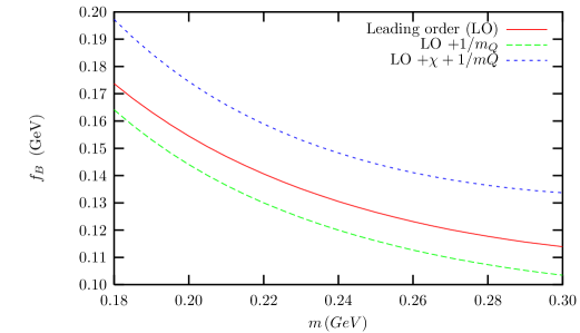
fig:Fb

Figure 10: $f_{B}$ as a function of $m$ for ${\langle}\,\overline{q}q\,{\rangle}^{1/3}$ = -240 MeV.

VI Applications

In this section we focus on the chiral quark model aspects, especially contributions proportional to the gluon condensate. There are always additional chiral loop corrections which can be found in BEF ; AHJOE ; ahjoeB ; EFH and references therein.

VI.1 $B\,-\,\overline{B}$ mixing and heavy quark effective theory

At quark level, the standard effective Lagrangian describing $B\,-\,\overline{B}$ mixing is EffHam

$${\cal L}_{eff}^{\Delta B=2}\,=\,-\,\frac{G_{F}^{2}}{4\pi^{2}}M_{W}^{2}\left(V_{tb}^{*}V_{tq}\right)^{2}\,S_{IL}\left(x_{t}\right)\,\eta_{B}\,b(\mu)\;Q_{B}\;,$$ (83)

where $G_{F}$ is Fermi’s coupling constant, the $V$’s are KM factors (for which $q=d$ or $s$ for $B_{d}$ and $B_{s}$ respectively) and $S_{IL}$ is the Inami-Lim function due to short distance electroweak loop effects for the box diagram. The quantity $Q_{B}\equiv Q(\Delta B=2)$ is a four quark operator

$$Q_{B}=\overline{q_{L}}\,\gamma^{\alpha}\,b_{L}\;\overline{q_{L}}\,\gamma_{\alpha}\,b_{L}\;,$$ (84)

where $q_{L}$ $(b_{L})$ is the left-handed projection of the $q$ $(b)$-quark field. The quantities $\eta_{B}=0.55\pm 0.01\,$ and $b(\mu)$ are calculated in perturbative quantum chromodynamics (QCD). At the renormalization scale $\mu~{}=~{}m_{b}$ $(\simeq 4.8~{}\text{GeV})$ one has $b(m_{b})\simeq 1.56$ in the naive dimension regularization scheme. The matrix element of the operator $Q_{B}$ between the meson states is parameterized by the bag parameter $B_{B_{q}}$ :

$${\langle}B|Q_{B}|\overline{B}{\rangle}{\equiv}\frac{2}{3}f_{B}^{2}M_{B}^{2}B_{B_{q}}(\mu)\;\,,$$ (85)

where by definition, $B_{B_{q}}=1$ within the factorized limit. In general, the matrix element of the operator $Q_{B}$ is dependent on $\mu$, and thereby $B_{B_{q}}$ also depends on $\mu$. As for $K-\overline{K}$ mixing, one defines a renormalization scale independent quantity

$$\hat{B}_{B_{q}}\equiv b(\mu)B_{B_{q}}(\mu)\;.$$ (86)

The $\Delta B=2$ operator in equation (84) can for $\Lambda_{\chi}<\mu<m_{b}$ be written gimenez ; mannel :

$$Q_{B}=\,C_{1}\,Q_{1}+C_{2}\,Q_{2}+\frac{1}{m_{b}}\sum_{i}\,h_{i}X_{i}\,+{\cal O}(1/m_{b}^{2})\;\,.$$ (87)

The operator $Q_{1}$ is $Q_{B}$ for $b$ replaced by $Q_{v}^{(\pm)}$, while $Q_{2}$ is generated within perturbative QCD for $\mu<m_{b}$. The operators $X_{i}$ are taking care of $1/m_{b}$ corrections. The quantities $C_{1},C_{2},h_{i}$ are Wilson coefficients. The operators are given by

$$Q_{1} =2\;\overline{q_{L}}\,\gamma^{\mu}\,Q^{(+)}_{v}\;\;\overline{q_{L}}\,\gamma_{\mu}\,Q^{(-)}_{v}\,\;,$$ (88)

$$Q_{2} =2\;\overline{q_{L}}\,v^{\mu}\,Q^{(+)}_{v}\;\;\overline{q_{L}}\,v_{\mu}\,Q^{(-)}_{v}\;\,,$$ (89)

$$X_{1} =2\;\overline{q_{L}}\,iD^{\mu}\,Q^{(+)}_{v}\;\overline{q_{L}}\,\gamma_{\mu}Q^{(-)}_{v}\ \;+......$$ (90)

The explicite expressions for the operators $X_{i}$ are given in ahjoeB . There are also non-local operators constructed as time-ordered products of $Q_{1,2}$ and the first order HQEFT Lagrangian in (46). The Wilson coefficients $C_{1}$ and $C_{2}$ have been calculated to NLO gimenez and for $\mu=\Lambda_{\chi}$ one has $C_{1}(\Lambda_{\chi})=1.22$ and $C_{2}(\Lambda_{\chi})=-0.15$. The coefficients $h_{i}$ have been calculated to leading order (LO) in mannel .

In order to find all the matrix element of $Q_{1,2}\,$, one uses the following relation between the generators of $SU(3)_{c}$ ($i,j,l,n$ are colour indices running from 1 to 3):

$$\delta_{ij}\delta_{ln}=\frac{1}{N_{c}}\delta_{in}\delta_{lj}\;+\;2\;t_{in}^{a}\;t_{lj}^{a}\;,$$ (91)

where $a$ is an index running over the eight gluon charges. This means that by means of a Fierz transformation, the operator $Q_{1}$ in (88) may also be written in the following way (there is a similar expression for $Q_{2}$):

$$Q_{1}^{F}\;=\;\frac{1}{N_{c}}Q_{1}\;+\;4\,\overline{q_{L}}\,t^{a}\,\gamma^{\mu}\,Q^{(+)}_{v}\,\overline{q_{L}}\,t^{a}\,\gamma_{\mu}\,Q^{(-)}_{v}\,.$$ (92)

The first (naive) step to calculate the matrix element of a four quark operator like $Q_{1}$ is to insert vacuum states between the two currents. This factorized limit means to bosonize the two currents in $Q_{1}$ and multiply them (see (56)). The second operator in (92) is genuinely non-factorizable. In the approximation where only the lowest gluon condensate is taken into account, the last term in (92) can be written in a quasi-factorizable way by bosonizating the heavy-light colour current with an extra colour matrix $t^{a}$ inserted and with an extra gluon emitted as shown in Fig. 11.

Figure 11: Non-factorizable soft gluonic contribution to the bag-parameter. (Here $\Gamma{\equiv}t^{a}\,\gamma^{\mu}\,L$.)

We find the bosonized colour current:

$$\left(\overline{q_{L}}t^{a}\,\gamma^{\alpha}Q_{v}^{(\pm)}\right)_{1G}\;\longrightarrow\;-\frac{G_{H}g_{s}}{8}\,G_{\mu\nu}^{a}\;Tr\left[\xi^{\dagger}\gamma^{\alpha}L\,H^{(\pm)}\left(\pm i\,I_{2}\left\{\sigma^{\mu\nu},\gamma\cdot v\right\}+\,\frac{1}{8\pi}\sigma^{\mu\nu}\right)\right]\;,$$ (93)

where $\{\,,\,\}$ symbolizes an anti-commutator. The result for the right part of the diagram with $\bar{B}$ replaced by $B$ is obtained by changing the sign of $v$ and letting ${P_{5}^{(+)}}\rightarrow{P_{5}^{(-)}}$. Multiplying the coloured currents, we obtain the non-factorizable parts of $Q_{1}$ and $Q_{2}$ to first order in the gluon condensate by using eq. (33).

Now the bag parameter can be extracted and may be written in the form:

$$\hat{B}_{B_{q}}=\frac{3}{4}\,\widetilde{b}\left[1+\frac{1}{N_{c}}(1-\delta_{G}^{B})+\frac{\tau_{b}}{m_{b}}+\frac{\tau_{\chi}}{32\pi^{2}f^{2}}\right]\;\,,$$ (94)

where the parameter $\widetilde{b}$ also involves the Wilson coefficients $C_{\gamma,v}$ defined in (21):

$$\widetilde{b}\;=\;b(m_{b})\,\left[\frac{C_{1}-C_{2}}{(C_{\gamma}+C_{v})^{2}}\right]_{\mu=\Lambda_{\chi}}\;.$$ (95)

The soft gluonic non-factorizable effects are given by

$$\delta_{G}^{B}\,=\,\frac{N_{c}{\langle}\frac{\alpha_{s}}{\pi}G^{2}{\rangle}}{32\pi^{2}f^{2}f_{B}^{2}}\,\frac{m}{M_{B}}\,\kappa_{B}\,\left[\frac{C_{1}}{C_{1}-C_{2}}\right]_{\mu=\Lambda_{\chi}}\;\ ,$$ (96)

where $\kappa_{B}$ is a dimensionless hadronic parameter which depends on $m,f,\mu_{G}^{2}$ and $g_{{\cal A}}$ and is of order 2. Note that we are qualitatively in agreement with Mel , where also a negative contribution to the bag factor from soft gluon effects is found. Numerically, $f$ and $f_{B}$ are of the same order of magnitude, and $\delta_{G}^{B}$ is therefore suppressed like $m/M_{B}$ compared to the corresponding quantity

$$\delta_{G}^{K}\,=\,N_{c}\frac{{\langle}\frac{\alpha_{s}}{\pi}G^{2}{\rangle}}{32\pi^{2}f^{4}}$$ (97)

found for $K-\overline{K}$ mixing BEF .

However, one should note that $f_{B}$ scales as $1/\sqrt{M_{B}}$ within HQEFT, and therefore $\delta_{G}^{B}$ is still formally of order $(m_{b})^{0}$. The quantity $\tau_{b}$ represents the $1/m_{b}$ corrections due to the operators $X_{i}$. Furthermore, the quantity $\tau_{\chi}$ represents the chiral corrections (including counterterms) to the bosonized versions of $Q_{1,2}$ ahjoeB . The bag parameter $\hat{B}$ is plotted as function of $m$ in Fig. 12 for the case $B_{s}$. Our results are numerically in agreement with lattice results latt .

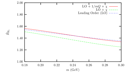
Figure 12: The bag parameter $\hat{B}$ for $B_{s}$ as a function of $m$.

VI.2 The processes $B\rightarrow D^{(*)}\overline{D^{(*)}}$

It has been observedEFH that the procseese $\bar{B}_{d,s}^{0}\to D_{s,d}\bar{D}_{s,d}$, $\bar{B}_{d,s}^{0}\to D^{*}_{s,d}\bar{D}_{s,d}$, $\bar{B}_{d,s}^{0}\to D_{s,d}\bar{D}_{s,d}^{*}$, and $\bar{B}_{d,s}^{0}\to D^{*}_{s,d}\bar{D}_{s,d}^{*}$, have no factorized contribution from the spectator mechanism. If one or two of the $D$-mesons in the final state are vectors, there are relatively small contributions from the annihilation mechanism. The effective non-leptonic Lagrangian at quark level has the usual form EffHam :

$${\mathcal{L}}_{W}=-4\frac{G_{F}}{\sqrt{2}}V_{cb}V_{cq}^{*}\sum_{i}a_{i}\;\hat{Q}_{i}(\mu)\;.$$ (98)

In our case there are only two numerically relevant operators (for $q=d,s$):

$$\hat{Q}_{1}=(\overline{q}_{L}\gamma^{\alpha}b_{L})\;(\overline{c}_{L}\gamma_{\alpha}c_{L})\;\;;\;\hat{Q}_{2}=(\overline{c}_{L}\gamma^{\alpha}b_{L})\;(\overline{q}_{L}\gamma_{\alpha}c_{L})\;.$$ (99)

At $\mu=m_{b}$, one has $a_{2}\sim 1$ and $a_{1}\sim 1/10$.

Using (91), we obtain the Fierzed version of the operators $\hat{Q}_{1,2}$:

$$\hat{Q}_{1}^{F}=\frac{1}{N_{c}}\hat{Q}_{2}+2(\overline{c}_{L}\gamma^{\alpha}t^{a}b_{L})\;(\overline{q}_{L}\gamma_{\alpha}t^{a}c_{L})$$

$$\hat{Q}_{2}^{F}=\frac{1}{N_{c}}\hat{Q}_{1}+2(\overline{q}_{L}\gamma^{\alpha}t^{a}b_{L})\;(\overline{c}_{L}\gamma_{\alpha}t^{a}c_{L})$$ (100)

The genuine non-factorizable $1/N_{c}$ chiral Lagrangian terms from “coloured quark operators” can be estimated within the $HL\chi QM$. However, in order to do this we have to treat the effective weak non-leptonic Lagrangian in (98) within heavy quark effective theory (HQEFT) neu . Then $b$, $c$, and $\overline{c}$ quarks are replaced by their corresponding operators in HQEFT:

$$b\rightarrow Q_{v_{b}}^{(+)}\quad,\;\,c\rightarrow Q_{v_{c}}^{(+)}\quad,\;\,\overline{c}\rightarrow Q_{\bar{v}}^{(-)}$$ (101)

up to $1/m_{b}$ and $1/m_{c}$ corrections. Then the effective weak non-leptonic Lagrangian (98) can be evolved down to the scale $\mu\sim\Lambda_{\chi}\sim$1 GeV GKMWF . At $\mu=1$ GeV we have $a_{2}\simeq 1.29+0.08i$, and $a_{1}\simeq-0.35-0.07i$. Note that $a_{1,2}$ are complex for $\Lambda_{\chi}<\mu<m_{c}$GKMWF .

Figure 13: Factorized contribution for $\overline{B^{0}}\rightarrow D^{+}D_{s}^{-}$ through the spectator mechanism, which does not exist for the decay mode $\overline{B^{0}}\rightarrow D_{s}^{+}D_{s}^{-}$. The double dashed lines represent heavy mesons, the double lines represent heavy quarks, and the single lines light quarks.

The bosonized factorized weak Lagrangian corresponding to Fig. 13 and the operator $\hat{Q}_{2}$ (with the dominating Wilson coefficient $a_{2}$) is obtained from (18), and (22), and (98):

$${\mathcal{L}}_{W-Fact}^{Bos}(Q_{2})=4\frac{G_{F}}{\sqrt{2}}V_{cb}V_{cq}^{*}(a_{2}+\frac{a_{1}}{N_{c}})\,\zeta(\omega)\frac{\alpha_{H}}{2}Tr\left[\overline{H_{c}^{(+)}}\gamma^{\alpha}LH_{b}^{(+)}\right]\cdot Tr\left[\xi^{\dagger}\gamma^{\alpha}LH_{\bar{c}}^{(-)}\right]\;,$$ (102)

where $\omega\equiv v_{b}\cdot v_{c}=v_{b}\cdot\bar{v}=M_{B}/(2M_{D})$. This Lagrangian (corresponding to the spectator mechanism) contributes to the factorized amplitude for the process $\overline{B^{0}}\rightarrow D^{+}D_{s}^{-}$, and is the starting point for chiral loop contributions of order $(m_{K}g_{{\cal A}}/4\pi f)^{2}$ (which are $1/N_{c}$ suppresed) to the processes $B\rightarrow D^{(*)}\overline{D^{(*)}}$.

Figure 14: Factorized contribution for $\overline{B^{0}}\rightarrow D_{s}^{+}D_{s}^{-}$ through the annihilation mechanism, which give zero contributions if both $D_{s}^{+}$ and $D_{s}^{-}$ are pseudo-scalars.

The bosonized factorized weak Lagrangian corresponding to Fig. 14 and the non-dominating Wilson coefficient $a_{1}$ is

$${\mathcal{L}}_{W-Fact}^{Bos}(Q_{1})=4\frac{G_{F}}{\sqrt{2}}V_{cb}V_{cq}^{*}(a_{1}+\frac{a_{2}}{N_{c}})\,\zeta(-\lambda)\frac{\alpha_{H}}{2}Tr\left[\xi^{\dagger}\gamma^{\mu}L\,H_{b}^{(+)}\right]\cdot Tr\left[\overline{H_{c}^{(+)}}\gamma^{\alpha}LH_{\bar{c}}^{(-)}\right]$$ (103)

where $\lambda\equiv\bar{v}\cdot v_{c}=(M_{B}^{2}/(2M_{D}^{2})-1)$. Unless one or both of the $D$-mesons in the final state are vector mesons, this matrix element is zero due to current conservation, which is analogous to the decay mode $\overline{D^{0}}\rightarrow K^{0}\overline{K^{0}}$ EFZ .

The genuine non-factorizable part for $\overline{B^{0}}\rightarrow D_{s}^{+}D_{s}^{-}$ at quark level can, by means of Fierz transformations and the identity (91), be written in terms of colour currents. The left part in Fig. 15 with gluon emission gives us the bosonized colour current which is the same as for $B-\overline{B}$ mixing in eq. (93).

Figure 15: Non-factorizable contribution for $\overline{B^{0}}\rightarrow D_{s}^{+}D_{s}^{-}$ through the annihilation mechanism with additional soft gluon emission. The wavy lines represent soft gluons ending in vacuum to make gluon condensates.

For the creation of a $D\bar{D}$ pair in the right part of Fig. 15, there is an analogue of (93), which can be written:

$$\left(\overline{Q_{v_{c}}^{(+)}}\,t^{a}\;\gamma^{\alpha}\,LQ_{\bar{v}}^{(-)}\right)_{1G}\;\;\longrightarrow\;\frac{G_{H}^{2}\,g_{s}}{32\pi m}\,G_{\mu\nu}^{a}\;Tr\left[\overline{H_{c}^{(+)}}\;\gamma^{\alpha}\,L\,H_{\bar{c}}^{(-)}X^{\mu\nu}\right]$$ (104)

where

$$X^{\mu\nu}\equiv\frac{r(-\lambda)}{\pi}\,\sigma^{\mu\nu}\,+\,\frac{1}{4(\lambda-1)}\left\{\sigma^{\mu\nu},\gamma\cdot t\right\}$$

and $\,t\equiv v_{c}-\bar{v}\,$ . Multiplying the currents and using (33) we obtain a bosonized effective Lagrangian as the product of two traces. Note that our non-factorizable amplitudes (proportional to the gluon condensate) are proportional to the numerically favourable Wilson coefficient $a_{2}$.

The gluon condensate contribution obtained from (93) and (104) is a linear combination of terms like:

$$Tr\left[\xi^{\dagger}\sigma^{\mu\alpha}L\,H_{b}^{(+)}\right]\cdot Tr\left[\overline{H_{c}^{(+)}}\gamma_{\alpha}LH_{\bar{c}}^{(-)}\gamma_{\mu}\right]\;,$$

$$Tr\left[\xi^{\dagger}\gamma^{\mu}L\,H_{b}^{(+)}\right]\cdot Tr\left[\overline{H_{c}^{(+)}}\gamma^{\alpha}LH_{\bar{c}}^{(-)}\sigma_{\mu\alpha}R\right]\;,$$

$$Tr\left[\xi^{\dagger}\gamma^{\mu}L\,H_{b}^{(+)}\right]\cdot Tr\left[\overline{H_{c}^{(+)}}\gamma_{5}LH_{\bar{c}}^{(-)}\gamma_{\mu}\right]\;,$$

$$Tr\left[\xi^{\dagger}L\,H_{b}^{(+)}\right]\cdot Tr\left[\overline{H_{c}^{(+)}}\gamma^{\alpha}LH_{\bar{c}}^{(-)}\gamma_{\alpha}\right]\;,$$

$$Tr\left[\xi^{\dagger}\sigma^{\mu\alpha}L\,H_{b}^{(+)}\right]\cdot Tr\left[\overline{H_{c}^{(+)}}\gamma_{\alpha}LH_{\bar{c}}^{(-)}\right](\bar{v}-v_{c})_{\mu}\;,$$

$$\varepsilon^{\mu\nu\alpha\lambda}(v_{c}+\bar{v})_{\nu}Tr\left[\xi^{\dagger}\gamma^{\mu}L\,H_{b}^{(+)}\right]\cdot Tr\left[\overline{H_{c}^{(+)}}\gamma^{\alpha}LH_{\bar{c}}^{(-)}\gamma_{\lambda}\right]\;.$$ (105)

These terms might have been written down based on the heavy quark symmetry, but the HL$\chi$QM selects a certain linear combination to be realized.

Our amplitudes for $B\to D\bar{D}$, in terms of chiral loop and gluon condensate contributions, are sensitive to $1/m_{c}$ corrections and counterterms which are not yet calculated EFH . Operators suppresssed by $1/m_{Q}$ are obtained by the replacements

$$Q_{v}^{(\pm)}\to\frac{1}{m_{Q}}i\gamma\cdot D_{\perp}Q_{v}^{(\pm)}\quad;\qquad D_{\perp}^{\nu}=D^{\nu}-v^{\nu}(v\cdot D)\;,$$ (106)

for one of the heavy quarks in (99) and (100). Some new quark operators of order $1/m_{Q}$ might also be generated by pQCD for $\mu<m_{Q}$. Counterterms correspond to mass insertion of $\widetilde{M}_{q}\,$, given by (17) and (29), at light quark lines in the diagrams for $B\to D\bar{D}$ this subsection.

VI.3 Other applications

Within the HL$\chi$QM, the process $B\rightarrow D\eta^{\prime}$ has been estimated EHP . This is done in two steps. First we calculate the subprocess $B\rightarrow Dgg^{*}$. Then the virtual gluon $g^{*}$ is attached to the $\eta^{\prime}gg^{*}$-vertex, and the other end in vacuum and make a gluon condensate together with one of the other soft gluons ($g$) from the $\eta^{\prime}gg^{*}$-vertex. Using Fierz transformations for the four quark operators for $b\rightarrow cd\bar{u}$, we obtain contributions corresponding to Fig. 16.

Figure 16: Gluon condensate contributions to $B\rightarrow D\eta^{\prime}$.

We have used existing parameterizations of the $\eta^{\prime}gg^{*}$-vertex form factor and assumed that the current for $B\rightarrow g^{*}$ is related to the better known case $B\rightarrow\rho$. It turns out that the “factorizable” diagram to the left in figure 16 can be neglected compared to the non-factorizable diagram to the right. For $m$ in the range 230-270 MeV, we obtained the result EHP $Br(B\rightarrow D\eta^{{}^{\prime}})\,=\,(2.2\,\pm\,0.4)\,\times\,10^{-4}\,$. Here $1/m_{Q}$ and chiral corrections are not included.

Heavy to light non-leptonic processes like $B,D\rightarrow K\pi$ cannot in general be treated within the HL$\chi$QM in its present form. (See, however, section VII-B). Still, semileptonic heavy to light processes might be treated at the “no recoil point” AHJOE . The form factors $f_{+}(q^{2})$ and $f_{-}(q^{2})$ are defined as:

$${\langle}\pi^{+}(p_{\pi})|\overline{u}\gamma^{\alpha}b|H{\rangle}\,=\,2\,{\langle}\pi^{+}(p_{\pi})|J_{f}^{\alpha}|H{\rangle}\,=\,f_{+}(q^{2})(p_{H}+p_{\pi})^{\alpha}\,+\,f_{-}(q^{2})(p_{H}-p_{\pi})^{\alpha}$$ (107)

where $p_{H}^{\alpha}=M_{H}v^{\alpha}$ and the index $a$ corresponds to quark flavour $u$ and $q^{\mu}=p_{H}^{\mu}-k_{\pi}^{\mu}$. The form factors get contributions from $J_{f}^{\alpha}(0)$ in (18) and $J_{f}^{\alpha}(1)$ in (58) close to the “no recoil point” where $v\cdot p_{\pi}$ is small:

$$f_{+}(q^{2})\,+\,f_{-}(q^{2}) = \frac{-1}{\sqrt{2M_{H}}f_{\pi}}\left(C_{\gamma}+C_{v}-g_{\cal A}C_{\gamma}\right)\alpha_{H}\;,$$ (108)

$$f_{+}(q^{2})\,-\,f_{-}(q^{2}) = -C_{\gamma}\frac{\sqrt{M_{H}}}{\sqrt{2}f_{\pi}}\left(\,\frac{g_{\cal A}\alpha_{H}}{v\cdot p_{\pi}}+\alpha_{H\gamma}^{(1)}\,\right)\;,$$ (109)

where we have neglected terms of first order in $v\cdot p_{\pi}$ (where $\alpha_{Hv}^{(1)}$ contributes). The $1/v\cdot p_{\pi}$ term in (109) is due to the $H^{*}$ pole. From equation (108) and (109) we see that

$$(f_{+}(q^{2})+f_{-}(q^{2}))/(f_{+}(q^{2})-f_{-}(q^{2}))\sim 1/M_{H}$$ (110)

which is the well known Isgur-Wise scaling law isgur2 . The equations for the two form factors $f_{+}$ and $f_{-}$ should be studied further, and chiral corrections and $1/m_{Q}$ corrections should be added.

VII Further possible extensions of chiral quark models

In this section we consider two possible extensions of chiral quark models which are not yet worked out in detail. The descriptions are therefore sketchy.

VII.1 Inclusion of light vectors

One might include vectors in the chiral perturbation theory EckDA and thus it should be possible to use the chiral quark model also in this case. We suggest a Lagrangian

$${\cal L}={\cal L}_{mass}+{\cal L}_{\chi QM}+{\cal L}_{IVA}\;,$$ (111)

where the interaction between quarks and the vectors and axial vectors is given by

$${\cal L}_{IVA}=\overline{\chi}\left[h_{V}\gamma^{\mu}V_{\mu}+h_{A}\gamma_{5}A_{\mu}\right]\chi\;.$$ (112)

Here $V$ are given as $\Pi$ in (6) with $\pi$ replaced by $\rho$ etc, and similarly for the axial vector $A$ where $\pi$ is replaced by $a_{1}$. The (bare) mass term is

$${\cal L}_{mass}=\bar{m}_{V}^{2}Tr\left[V_{\mu}V^{\mu}\right]+\bar{m}_{A}^{2}Tr\left[A_{\mu}A^{\mu}\right]\;.$$ (113)

After quarks are integrated out, the masses are modified and identified with the physical ones. Then a kinetic term is also generated:

$${\cal L}_{kin}=-\frac{1}{2}\left[V_{\mu\nu}V^{\mu\nu}\right]\,-\,\frac{1}{2}\left[A_{\mu\nu}A^{\mu\nu}\right]\;;$$ (114)

where for $X=V,A$:

$$X_{\mu\nu}\,=\,\nabla_{\mu}X_{\nu}\,-\,\nabla_{\nu}X_{\mu}\;,$$ (115)

and similar for the axial vector. Here $\nabla$ is a covariant derivative including the goldstones:

$$\nabla_{\mu}X_{\nu}\,\equiv\partial_{\mu}X_{\nu}\,+\,i\,[{\cal V}_{\mu},X_{\nu}]\;.$$ (116)

For the left-handed current for $vac\rightarrow X=V,A$ we find the $SU(3)$ octet current

$$J_{\mu}^{n}(vac\rightarrow X)=\frac{1}{2}k_{X}Tr\left[\Lambda^{n}X_{\mu}\right]\;,$$ (117)

where the quantity $\Lambda^{n}$ is given by (39).

As previuosly, bosonization gives constraints on the parameters of the vectorial sector. From normalization of the kinetic term(s) we obtain:

$$\frac{f^{2}h_{V}^{2}}{3m^{2}}\left[1\,-\,\frac{1}{15m^{2}f^{2}}{\langle}\frac{\alpha_{s}}{\pi}G^{2}{\rangle}\right]\,=\,1\;,$$ (118)

where $h_{A}=h_{V}$ before chiral corrections. For the currents we obtain

$$k_{V}\,=\,\frac{1}{2}h_{V}\left(-\frac{{\langle}\,\overline{q}q\,{\rangle}}{m}+f^{2}-\frac{1}{8m^{2}}{\langle}\frac{\alpha_{s}}{\pi}G^{2}{\rangle}\right]\;,$$ (119)

and similarly , for the axial case:

$$k_{A}\,=\,\frac{1}{2}h_{A}\left(-\frac{{\langle}\,\overline{q}q\,{\rangle}}{m}-3f^{2}+\frac{1}{8m^{2}}{\langle}\frac{\alpha_{s}}{\pi}G^{2}{\rangle}\right]\;.$$ (120)

The formalism suggested in this subsection might for instance, when combined with HL$\chi$QM, give a reasonable description of the weak current for $D$-meson decays $D\rightarrow V$ Svjet . This might also be the case for processes like $D\rightarrow VP$, where $V$ is a vector meson and $P$ is a pseudoscalar. In the last case, non-factorizable contributions can be calculated in terms of chiral loops and gluon condensates. However, one should keep in mind that a limitation in this case is that $V$ is (also formally) light compared to $D$.

VII.2 Heavy to light transitions

As emphasized in the introduction, the HL$\chi$QM is not suited to describe $B\rightarrow\pi$ transitions except for semileptonic transitions close to the no recoil point. It might therefore be surprising that we consider a formalism for chiral perturbation theory for $B\rightarrow\pi$ transitions (and more general $B\rightarrow P$ for $P=\pi,K,\eta$), because the involved pion is hard. However, in general, in a transition $B\rightarrow$ pions, we might have a configuration where one pion is hard and one (or more) is soft. For such cases we split the pseudoscalar sector in hard and soft pseudoscalars. The soft pseudoscalars are represented as before , while the hard pseudoscalars are represented by an octet 3$\times$3 matrix $M$ given as $\Pi$ in eq. (6), but transforming as $\Sigma$ under $SU(3)_{L}\times SU(3)_{R}$.

Starting with a $\gamma_{5}$ coupling for quarks coupling to pseudoscalars, we represent the hard light quark with a quark field $q_{n}$ LEET ; SCET and the soft light quarks by the flavour rotated fields $\chi$ in section III. Then we arrive at an interaction Lagrangian

$${\cal L}_{n}=G_{M}\bar{\chi}\left[\xi^{\dagger}MR-\xi M^{\dagger}L\right]q_{n}\;,$$ (121)

for a hard light quark $q_{n}$ entering a hard pion (kaon) with momentum $p_{M}=E\,n$ where $n$ is a lightlike vector and $E$ is the energy of the hard pion(kaon). The hard quark has then momentum $p_{q}=E\,n+k$, where $k$ is of order $\Lambda_{\chi}\sim$ 1 GeV or smaller. $G_{M}$ is a coupling which has to be determined by some physical requirements. For an outgoing hard quark we have

$${\cal L}_{\bar{n}}=G_{M}\bar{q_{n}}\left[M\xi^{\dagger}R-M^{\dagger}\xi L\right]\chi\;.$$ (122)

Now one might combine (121) and (122) with HL$\chi$QM and use some version of a large energy effective field theory (LEET) LEET to describe the light hard quarks. Using the LEET propagator

$$\frac{\gamma\cdot n}{2n\cdot k}$$ (123)

for the light hard quark, we can write down a quark loop diagram for $B\rightarrow P$ with a corresponding amplitude for the heavy-light weak current (to leading order)

$$J_{k}^{\alpha}(B\rightarrow P)\;=\;K\,Tr\left[\Gamma^{\alpha}H_{vh}\gamma\cdot n\,\xi M^{\dagger}\right]\;.$$ (124)

Given the transformation properties in (10), (15), and (27), the current (124) transforms as in (19).

The behaviour of the quantity (form factor) $K$ is known from theoretical considerations within LEETLEET and soft collinear effective theory (SCET)SCET :

$$K\;\sim\;E\,\zeta^{(v)}(M_{B},E)\;,$$ (125)

where $\zeta^{(v)}$ is expected to scale as

$$\zeta^{(v)}(M_{B},E)\;\sim\;\frac{\sqrt{M_{B}}}{E^{2}}\;.$$ (126)

Note that a factor $\sqrt{M_{B}}$ is associated with the heavy ($B$) meson wave function and similarly a factor $\sqrt{E}$ with the wave function of the hard pseudoscalar meson. Within our framework, $K$ will contain the product of the couplings $G_{H}$ and $G_{M}$, and some loop integrals involving the heavy quark propagator, the ordinary Dirac propagator for the soft quark, and the LEET propagator in (123). However, it has been pointed out that the LEET propagator is too singular to give meaningful loop integralsUglea , and that the LEET is incompleteSCET . Therefore the simple expression in (123) has to be modified in some way, by keeping $n^{\mu}n_{\mu}=\delta^{2}\neq 0$ with $\delta\sim 1/E$, by adding a small quantity in the LEET propagator denominator, or by modifying the formalism in other ways. And this modification has to be done such that one does not come in conflict with the known scaling properties of $\zeta^{(v)}$. Keeping $\delta\neq 0$ and $\delta\sim 1/E$, some of the involved loop integrals have the same mathematical form as those involved in the Isgur-Wise function in (73), but with $\omega\to 1/\delta$. The most plausible scenario is that $G_{M}\sim E^{-3/2}$. Anyway, knowledge of $\zeta^{(v)}$ will put restrictions on $G_{M}$.

The $W\rightarrow\pi$ transition is in BBNS ; SCET represented by an integral over a momentum distribution proportional to $x(1-x)$ dominated at $x\sim 1/2$. However, there are also suppressed contributions (for $E>>\Lambda_{\chi}$) from momentum configurations where one quark (anti-quark) is hard and the anti-quark (quark) is soft. The left-handed current is in this case given by

$$j^{l}_{\mu}\;=\bar{q}_{n}\,\gamma_{\mu}L\,(\lambda^{l}\xi)\,\chi\quad,\quad\text{or}\;\qquad j^{l}_{\mu}\;=\bar{\chi}\,(\xi^{\dagger}\lambda^{l})\,\gamma_{\mu}L\,q_{n}\;,$$ (127)

where $l$ is an $SU(3)$ octet index. These quark currents will, when combined with (121) and (122), generate a bosonized current

$$\Delta J^{l}_{\mu}\,=\;N\,\tilde{n}^{\mu}Tr\left[\lambda^{l}(\Sigma M^{\dagger}+M\Sigma^{\dagger})\right]\;,$$ (128)

where $\tilde{n}$ is another (almost) lightlike vector with opposite three momentum compared to $n$ such that $\tilde{n}^{2}=\delta^{2}$ and $\tilde{n}\cdot n=2-\delta^{2}$. In the most plausible scenario mentioned above $N$ scales as a constant ($E^{0}$), which is suppressed by $1/E$ compared with the leading order current $\sim E\,f^{(0)}_{P}\,\tilde{n}^{\mu}$. The physical decay constant $f_{P}$ (for $P=\pi,K,\eta$) is within this scheme given by $f^{(0)}_{P}$ plus the suppressed contribution $\sim N/E$ from (128).

Now, the product of the currents in (124) and (128) will give a factorized $1/E$ suppressed contribution to $B\rightarrow K\pi$ corresponding to the diagram in Fig. 13, with $\bar{c}$ and $c$ replaced by energetic (anti) quarks, $D$ by $\pi$ and $D_{s}$ by $K$. This contribution can of course not be distinguished from the standard factorized contribution. However, pulling out soft pseudoscalars from $\xi$ and $\Sigma$ in the currents (124) and (128), we obtain $1/E$ suppressed non-factorizable chiral loop contributions to $B\rightarrow K\pi$. Similarly there will be $1/E$ suppressed gluon condensate contributions. Such suppressed terms are not in conflict with QCD factorization BBNS .

VIII Conclusion

We have presented the main features of chiral quark models, both in the pure light and the heavy-light sector. Especially, the HL$\chi$QM seem to work well. In that case, it is possible to systematically calculate the $1/m_{Q}$ corrections as well as chiral corrections. The model may be used to give predictions for many quantities. Especially, it is suitable for calculation of the $B$-parameter for $B-\bar{B}$ mixing AHJOE , and for a study of processes of the type $B\rightarrow D\bar{D}$. For heavy to light transitions ($B\rightarrow K\pi$, say) the HL$\chi$QM cannot be used in its present form. It remains to be seen if the extension indicated in sect VII-B to incorporate light energetic quarks will lead to some understanding of such decays.

In our version of the chiral quark models(pure light and heavy light cases) soft gluon effects are truncated to include only the secord order gluon condensate. It has worked reasonably well up to now, but one may wonder if this is enogh to accomodate all effects, for instance when light vectors are included. Maybe for instance higher order gluon condensates could be included, but our simple model will of course then be much more complicated.