JLAB-THY-04-42

${\rm ECT}^{*}$-04-11

Direct $\boldsymbol{CP}$ Violation, Branching Ratios and Form Factors $\boldsymbol{B\rightarrow\pi}$, $\boldsymbol{B\rightarrow K}$ in $\boldsymbol{B}$ Decays

O. Leitner¹, X.-H. Guo², A.W. Thomas^3
1 ${\rm{ECT}}^{*}$, Strada delle Tabarelle, 286, 38050 Villazzano (Trento), Italy

² Key Laboratory of Radiation Beam Technology and Material Modification of National Ministry of Education, and Institute of Low Energy Nuclear Physics, Beijing Normal University, Beijing 100875, China

³ Jefferson Lab, 12000 Jefferson Avenue, Newport News, VA 23606, USA

The $B\to\pi$ and $B\to K$ transitions involved in hadronic $B$ decays are investigated in a phenomenological way through the framework of QCD factorization. By comparing our results with experimental branching ratios from the BELLE, BABAR and CLEO Collaborations for all the $B$ decays including either a pion or a kaon, we propose boundaries for the transition form factors $B\to\pi$ and $B\to K$ depending on the CKM matrix element parameters $\rho$ and $\eta$. From this analysis, the form factors required to reproduce the experimental data for branching ratios are $F^{B\to\pi}=0.31\pm 0.12$ and $F^{B\to K}=0.37\pm 0.13$. We calculate the direct $CP$ violating asymmetry parameter, $a_{CP}$, for $B\to\pi^{+}\pi^{-}\pi$ and $B\to\pi^{+}\pi^{-}K$ decays, in the case where $\rho-\omega$ mixing effects are taken into account. Based on these results, we find that the direct $CP$ asymmetry for $B^{-}\to\pi^{+}\pi^{-}\pi^{-}$, $\bar{B}^{0}\to\pi^{+}\pi^{-}\pi^{0}$, $B^{-}\to\pi^{+}\pi^{-}K^{-}$, and $\bar{B}^{0}\to\pi^{+}\pi^{-}\bar{K}^{0}$, reaches its maximum when the invariant mass $\pi^{+}\pi^{-}$ is in the vicinity of the $\omega$ meson mass. The inclusion of $\rho-\omega$ mixing provides an opportunity to erase, without ambiguity, the phase uncertainty mod$(\pi)$ in the determination of the CKM angles $\alpha$ in case of $b\to u$ and $\gamma$ in case of $b\to s$.

PACS Numbers: 11.30.Er, 12.39.-x, 13.25.Hw.
Keywords: CP violation, branching ratio, form factor

1 Introduction

The violation of $CP$ symmetry in the framework of the Standard Model is supposed to arise from the well-known Cabibbo-Kobayashi-Maskawa (CKM) [1, 2] matrix through a “weak” phase, $\phi$. This matrix is based on the quark flavors, charged currents and weak interaction properties within the Standard Model. In order to make that picture as accurate as possible and to look for complementary insight from New Physics (NP), $B$ meson decays [3, 4, 5] have been investigated extensively, for many years, in both experimental and theoretical ways.

On the experimental side, branching ratios (of order $O(10^{-6})$) for $B$ charmless or charm (exclusive non leptonic) decays have been measured more and more accurately thanks to three main $e^{+}e^{-}$ colliders (list non exhaustive) operating at the $\Upsilon(4S)$ resonance: CLEO (symmetric-energy $B$-factory), BELLE and BABAR (asymmetric-energy $B$-factories). Despite a small number of discrepancies in some of the measurements of branching ratios, these $B$-facilities provide direct and/or indirect constraints on the unitarity triangle (UT) parameters $\rho$ and $\eta$. The latter parameters (known at the level of accuracy of $10\%$) are the corner stone of the whole $CP$ violation theory. They are subject to tremendous efforts into their experimental determination since all of the $B$-branching ratios ($CP$ violating asymmetries as well) are directly related to them within the theoretical formalism. The experimental determination of $CP$ violation (direct or indirect) is not as easy as for branching ratios because of the competition (sum or difference) between different topologies suffering from large hadronic uncertainties. However, since its discovery in neutral kaon decay in 1964 [6] and in neutral $B$ decay in 2001 [7, 8], its measurement has been regularly improved. The main quantities which are directly measured are $\epsilon,\epsilon^{\prime}$ for kaon decays and $\sin 2\alpha,\sin 2\beta$ for $B$ decays. Altogether they mainly restrict the allowed range of values [9] for the parameters $\rho$ and $\eta$ [$0.077<\rho<0.266,\;\;0.298<\eta<0.406$ at 95% confidence level and $0.130<\rho<0.226,\;\;0.324<\eta<0.377$ at 68% confidence level].

On the theoretical side, direct $CP$ violating asymmetries in $B$ decays occur through the interference of, at least, two amplitudes with different weak phase, $\phi$, and strong phase, $\delta$. The extraction of the weak phase $\phi$ (which is determined by a combination of CKM matrix elements) is made through the measurement of a $CP$ violating asymmetry. However, one must know the strong phase $\delta$ which is not still well determined in any theoretical framework. $B$ non-leptonic decay amplitudes involve hadronic matrix elements, $\langle M_{1}M_{2}|O_{i}|B\rangle$, and their computation is not trivial since it requires that one factorizes hadronic matrix elements of four quark operators. Assuming that they are saturated by a vacuum intermediate state, it reduces to the product of two matrix elements of two quark currents, corresponding to the weak transition form factor for $B\rightarrow M_{1}$ ($M_{2}$) and the decay constant of $M_{2}$ ($M_{1}$). In addition to this “naive” image (naive factorization) [10, 11, 12] justified in the large $N_{c}$-limit, radiative non-factorizable corrections (at order $O(\alpha_{s})$) coming from the light quark spectator of the $B$ meson are included in the QCD factorization [13, 14, 15, 16, 17, 18, 19, 20, 21] framework, where the main uncertainty comes from the $O(\Lambda_{QCD}/m_{B})$ terms.

It is known that in order to have a large signal for $CP$ violation, we have to appeal to some phenomenological mechanism to obtain a large strong phase $\delta$. In this regard, the isospin symmetry violating mixing between $\rho^{0}$ and $\omega$ can be extremely important, since it can lead to a large $CP$ violation in $B$ decays such as $B\to\rho^{0}(\omega)Y\to\pi^{+}\pi^{-}Y$ ($Y$ defines a meson) because the strong phase passes through $90^{o}$ at the $\omega$ resonance [28, 29, 30, 31]. In addition, as the $\omega$ is very narrow, one is essentially guaranteed that the strong phase will pass through $\pi/2$ very close to the $\omega$-mass regardless of other background sources of strong phase.

In this paper, we first investigate in a phenomenological way, the dependence on the form factors $F^{B\to\pi}$ and $F^{B\to K}$ of all the branching ratios for $B$ decaying into $\pi X$ or $KX$, where $X$ is either a pseudo-scalar ($\pi,K,\eta^{(\prime)}$), or a vector ($\rho,\omega,K^{*},\phi$) meson. At the same time, we determine, by making comparison between experimental and theoretical results, a range of values for the hard-scattering (annihilation) phases, $\varphi_{H}(\varphi_{A})$ and parameters $\varrho_{H}(\varrho_{A})$, respectively. These phases, $\varphi_{H,A}$, and parameters, $\varrho_{H,A}$, arise in QCD factorization because of divergent endpoint integrals when the hard scattering and annihilation contributions are calculated. The analysis is performed using all the latest data for $b\to s$ and $b\to u$ transitions, concentrating on the CLEO, BABAR and BELLE branching ratio results. Based on this investigation, we study the sign of $\sin\delta$, the ratio between tree and penguin contributions and finally the direct $CP$ violating asymmetry in $B$ decays such as $B\to\pi^{+}\pi^{-}Y$, where $Y=\{\pi^{0,\pm},K^{0,\pm}\}$.

The reminder of this paper is organized as it follows. In section 2, we present the form of the low energy effective Hamiltonian based on the operator product expansion. In section 3 we recall the naive factorization procedure and give the QCD factorization formalism based on an expansion of naive factorization in term of $\Lambda_{QCD}/m_{B}$. Section 4 focuses on the $\rho^{0}-\omega$, $\eta-\eta^{\prime}$ mixing schemes as well as on the $CP$ violation formalism. In sections 5 and 6, the CKM matrix and all the necessary input parameters (form factor, decay constant, masses) are discussed in detail, respectively. The following section is devoted to results and discussions for $B$ branching ratios and direct $CP$ violating asymmetries. Finally, in the last section, we draw some conclusions.

2 Effective Hamiltonian

In any phenomenological treatment of the weak decays of hadrons, the starting point is the weak effective Hamiltonian at low energy [32, 33, 34, 35, 36]. It is obtained by integrating out the heavy fields (e.g. the top quark, $W^{\pm}$ and $Z$ bosons) from the Standard Model Lagrangian. It can be written as,

$${\cal H}_{eff}^{\bigtriangleup B=1}=\frac{G_{F}}{\sqrt{2}}\sum_{i}V_{CKM}C_{i}(\mu)O_{i}(\mu)\ ,$$ (1)

where $G_{F}$ is the Fermi constant, $V_{CKM}$ is the CKM matrix element, $C_{i}(\mu)$ are the Wilson coefficients, $O_{i}(\mu)$ are the operators entering the Operator Product Expansion (OPE) and $\mu$ represents the renormalization scale. In the present case, since we take into account both tree and penguin operators, the matrix elements of the effective weak Hamiltonian reads as,

$$\langle M_{1}M_{2}|{\cal H}_{eff}^{\bigtriangleup B=1}|B\rangle=\\ \frac{G_{F}}{\sqrt{2}}\Biggl{[}V_{ub}V_{uq}^{*}\sum_{i=1}^{2}C_{i}(\mu)\langle M_{1}M_{2}|O_{i}^{q}|B\rangle(\mu)-V_{tb}V_{tq}^{*}\sum_{i=3}^{10}C_{i}(\mu)\langle M_{1}M_{2}|O_{i}|B\rangle(\mu)\Biggr{]}+h.c.\ ,$$ (2)

where $q=d\;{\rm or}\;s$ according to the transition $b\to u$ or $b\to s$. $\langle M_{1}M_{2}|O_{i}|B\rangle$ are the hadronic matrix elements, and $M_{i}M_{j}$ indicates either a pseudo-scalar and a vector in the final state, or two pseudo-scalar mesons in the final state. The matrix elements describe the transition between initial and final states at scales lower than $\mu$ and include, up to now, the main uncertainties in the calculation because they involve non-perturbative physics. The Operator Product Expansion is used to separate the calculation of the amplitude, $A(M\rightarrow F)\propto C_{i}(\mu)\langle F|O_{i}|M\rangle(\mu)$, into two distinct physical regimes. One is called hard or short-distance physics, represented by $C_{i}(\mu)$ and calculated by a perturbative approach. The other is called soft or long-distance physics. This part is described by $O_{i}(\mu)$, and is derived by using a non-perturbative approach such as the $1/N_{c}$ expansion [37], QCD sum rules [38, 39] or hadronic sum rules.

The operators, $O_{i}(\mu)$, can be understood as local operators which govern effectively a given decay, reproducing the weak interaction of quarks in a point-like approximation. The definitions of the operators $O_{i}$ [32, 33, 34] are recalled for completeness,
- Current-current operators:

$$O_{1}^{p}= (\bar{p}_{\alpha}b_{\alpha})_{V-A}(\bar{q}_{\beta}p_{\beta})_{V-A}\ ,\hskip 46.94687pt O^{p}_{2}=(\bar{p}_{\alpha}b_{\beta})_{V-A}(\bar{q}_{\beta}p_{\alpha})_{V-A}\ ,$$ (3)

- QCD-penguin operators:

$$O_{3}= (\bar{q}_{\alpha}b_{\alpha})_{V-A}\sum{}_{\!q^{\prime}}\,(\bar{q}^{\prime}_{\beta}q_{\beta})_{V-A}\ ,\hskip 19.91684pt O_{4}=(\bar{q}_{\alpha}b_{\beta})_{V-A}\sum{}_{\!q^{\prime}}\,(\bar{q}^{\prime}_{\beta}q_{\alpha})_{V-A}\ ,$$

$$O_{5}= (\bar{q}_{\alpha}b_{\alpha})_{V-A}\sum{}_{\!q^{\prime}}\,(\bar{q}^{\prime}_{\beta}q_{\beta})_{V+A}\ ,\hskip 19.91684pt O_{6}=(\bar{q}_{\alpha}b_{\beta})_{V-A}\sum{}_{\!q^{\prime}}\,(\bar{q}^{\prime}_{\beta}q_{\alpha})_{V+A}\ ,$$ (4)

- Electroweak penguin operators:

$$O_{7}= (\bar{q}_{\alpha}b_{\alpha})_{V-A}\sum{}_{\!q^{\prime}}\,{\textstyle\frac{3}{2}}e_{q}^{\prime}(\bar{q}^{\prime}_{\beta}q_{\beta})_{V+A}\ ,\hskip 2.56064pt O_{8}=(\bar{q}_{\alpha}b_{\beta})_{V-A}\sum{}_{\!q^{\prime}}\,{\textstyle\frac{3}{2}}e_{q}^{\prime}(\bar{q}^{\prime}_{\beta}q_{\alpha})_{V+A}\ ,$$

$$O_{9}= (\bar{q}_{\alpha}b_{\alpha})_{V-A}\sum{}_{\!q^{\prime}}\,{\textstyle\frac{3}{2}}e_{q}^{\prime}(\bar{q}^{\prime}_{\beta}q_{\beta})_{V-A}\ ,\hskip 2.84544pt O_{10}=(\bar{q}_{\alpha}b_{\beta})_{V-A}\sum{}_{\!q^{\prime}}\,{\textstyle\frac{3}{2}}e_{q}^{\prime}(\bar{q}^{\prime}_{\beta}q_{\alpha})_{V-A}\ ,$$ (5)

where $(\bar{q}_{1}q_{2})_{V\pm A}=\bar{q}_{1}\gamma_{\mu}(1\pm\gamma_{5})q_{2}$, $\alpha,\beta$ are colour indices, $e_{q}^{\prime}$ are the electric charges of the quarks in units of $|e|$, and a summation over all the active quarks, $q^{\prime}=u,d,s,c$, is implied. In Eq. (3) $p$ denotes the quark $u$ or $c$ and $q$ denotes the quark $u$ or $s$, according to the given transition $b\to u$ or $b\to s$. Finally, expressions for the operators $O_{7\gamma}$ and $O_{8g}$ are,

$$O_{7\gamma} = \frac{-e}{8\pi^{2}}\,m_{b}\,\bar{s}\sigma_{\mu\nu}(1+\gamma_{5})F^{\mu\nu}b\ ,$$

$$O_{8g} = \frac{-g_{s}}{8\pi^{2}}\,m_{b}\,\bar{s}\sigma_{\mu\nu}(1+\gamma_{5})G^{\mu\nu}b\ .$$ (6)

In Eq. (6) the definition of the dipole operators $O_{7\gamma}$ and $O_{8g}$ corresponds to the sign convention applied for the gauge-covariant derivative, $iD^{\mu}=i\delta^{\mu}+g_{s}A^{\mu}_{a}t_{a}$.

The Wilson coefficients [33], $C_{i}(\mu)$, represent the physical contributions from scales higher than $\mu$ (through OPE one can separate short-distance and long-distance contributions). Since QCD has the property of asymptotic freedom, they can be calculated in perturbation theory. The Wilson coefficients include the contributions of all heavy particles, such as the top quark, the $W^{\pm}$ bosons, and the charged Higgs boson. Usually, the scale $\mu$ is chosen to be of order ${\cal O}(m_{b})$ for $B$ decays. Their calculation will be discussed in the following section.

3 Factorization

3.1 Naive factorization

The computation of the hadronic matrix elements, $\langle M_{1}M_{2}|O_{i}|B\rangle$, is not trivial and requires some assumptions. The first general method is the so-called “factorization” procedure [10, 11, 12], in which one approximates the matrix element as a product of a transition matrix element between a $B$ meson and one final state meson and a matrix element which describes the creation of the second meson from the vacuum. In other words, the hadronic matrix elements are expressed in terms of form factor, $F^{B\to M_{i}}$, times decay constant, $f_{M_{j}}$. This can be formulated as,

$$\langle M_{1}M_{2}|O_{i}|B\rangle= \langle M_{1}|J_{2i}^{\mu}|0\rangle\ \langle M_{2}|J_{\mu,1i}|B\rangle\propto f_{M_{1}}F^{B\to M_{2}}\ ,$$

$${\rm or}\;\;\langle M_{1}M_{2}|O_{i}|B\rangle= \langle M_{2}|J_{4i}^{\mu}|0\rangle\ \langle M_{1}|J_{\mu,3i}|B\rangle\propto f_{M_{2}}F^{B\to M_{1}}\ ,$$ (7)

where the $J_{\mu,ji}$ are the transition currents such as $\bar{q}_{j}\gamma_{\mu}(1-\gamma_{5})q_{i}$. This approach is known as naive factorization since it factorizes $\langle M_{1}M_{2}|O_{i}|B\rangle$ into a simple product of two quark matrix elements. Therefore, the amplitude for a given decay can be finally written as,

$$A(B\rightarrow M_{1}M_{2})\propto\frac{G_{F}}{\sqrt{2}}\Biggl{[}\sum_{i=1}^{10}V_{CKM}C_{i}(\mu)\langle M_{1}M_{2}|O_{i}|B\rangle(\mu)\Biggr{]}\\ \propto\frac{G_{F}}{\sqrt{2}}\Biggl{[}\sum_{i=1}^{10}V_{CKM}C_{i}(\mu)\langle M_{1}|J_{2i}^{\mu}|0\rangle\langle M_{2}|J_{\mu,1i}|B\rangle\Biggr{]}\ .$$ (8)

A possible justification for this approximation has been given by Bjorken [40]: the heavy quark decays are very energetic, so the quark-antiquark pair in a meson in the final state moves very fast away from the localized weak interaction. The hadronization of the quark-antiquark pair occurs far away from the remaining quarks. Then, the meson can be factorized out and the interaction between the quark pair in the meson and the remaining quark is tiny.

The main uncertainty in this approach is that the final state interactions (FSI) are neglected. Corrections associated with the factorization hypothesis are parameterized and hence there may be large uncertainties [41]. Moreover, the $\mu$-scale dependence of the amplitude does not match on the two sides of Eq. (8). Finally, the lack of a dynamical mechanism for creating a strong phase may lead to discrepancies in comparison with experimental data. In spite of this, there are indications that the approach should give, at least, a good estimate of the magnitude of the $B$ decay amplitude in many cases [42, 43].

Working in the Quark Model scheme, the matrix elements for $B\to M_{i}$ and $B\to M_{i}^{*}$ (where $M_{i}$ and $M_{i}^{*}$ denote pseudo-scalar and vector mesons, respectively) can be decomposed as follows for the pseudo-scalar-pseudo-scalar transition [44, 45]:

$${\langle M_{i}|J_{\mu}|B\rangle}=\left(p_{B}+p_{M_{i}}-\frac{m_{B}^{2}-m_{M_{i}}^{2}}{k^{2}}k\right)_{\mu}{F_{1}(k^{2})}+\frac{m_{B}^{2}-m_{M_{i}}^{2}}{k^{2}}k_{\mu}{F_{0}(k^{2})}\ ,$$ (9)

where $J_{\mu}$ is the weak current defined as $J_{\mu}=\bar{q}\gamma_{\mu}(1-\gamma_{5})b$ with $q={u,d,s}$ and $k=P_{B}-P_{M_{i}(M_{i}^{*})}$. $F_{0},F_{1}$ are the form factors related to the transition $0^{-}\to 0^{-}$. In the helicity basis, they represent, respectively, the transition amplitudes corresponding to the exchange of a vector and a scalar boson in the t-channel. For the vector transition, one has:

$${\langle M^{\star}_{i}|J_{\mu}|B\rangle}=\frac{2}{m_{B}+m_{M_{i}^{\star}}}\epsilon_{\mu\nu\rho\sigma}\epsilon^{\star\nu}p_{B}^{\rho}p_{M_{i}^{\star}}^{\sigma}{V(k^{2})}+i\Biggl{\{}\epsilon_{\mu}^{\star}(m_{B}+m_{M_{i}^{\star}}){A_{1}(k^{2})}\\ -\frac{\epsilon^{\star}\cdot k}{m_{B}+m_{M_{i}^{\star}}}(P_{B}+P_{M_{i}^{\star}})_{\mu}{A_{2}(k^{2})}-\frac{\epsilon^{\star}\cdot k}{k^{2}}2m_{M_{i}^{\star}}\cdot k_{\mu}{A_{3}(k^{2})}\Biggr{\}}\\ +i\frac{\epsilon^{\star}\cdot k}{k^{2}}2m_{M_{i}^{\star}}\cdot k_{\mu}{A_{0}(k^{2})}\ ,$$ (10)

where $\epsilon_{\mu}$ is the polarization of $M_{i}^{*}$ with the condition $\epsilon_{\mu}\cdot P_{M_{i}^{*}}^{\mu}=0$. $A_{0},A_{1},A_{2},A_{3}$ and $V$ are the form factors which describe the axial and vector transitions $0^{-}\to 1^{-}$, respectively. $A_{1}(k^{2})$ and $A_{2}(k^{2})$ are related to the $1^{+}$ intermediate states whereas $A_{0}(k^{2})$ refers to the $0^{+}$ state. As regards $V(k^{2})$, it can be understood as the $1^{-}$ intermediate state in the transition $0^{-}\to 1^{-}$. Finally, in order to cancel the poles at $k^{2}=0$, the form factors respect the conditions:

$$F_{1}(0)=F_{0}(0),\;\;A_{3}(0)=A_{0}(0)\ ,$$ (11)

as well as the following relation:

$$A_{3}(k^{2})=\frac{m_{B}+m_{M_{i}^{\star}}}{2m_{M_{i}^{\star}}}A_{1}(k^{2})-\frac{m_{B}-m_{M_{i}^{\star}}}{2m_{M_{i}^{\star}}}A_{2}(k^{2})\ .$$ (12)

Regarding the matrix element $\langle M_{i}(q)|\bar{q}_{1}\gamma_{\mu}(1-\gamma_{5})q_{2}|0\rangle$, it simplifies as follows:

$${\langle M_{i}(q)|\bar{q}_{1}\gamma_{\mu}\gamma_{5}q_{2}|0\rangle} =-if_{P}q_{\mu}\ ,\;\;{\rm for\;\;a\;pseudo\!\!-\!\!scalar\;\;meson}\ ,$$

$${\langle M_{i}(q)|\bar{q}_{1}\gamma_{\mu}q_{2}|0\rangle} =f_{V}m_{V}\epsilon_{\mu}\ ,\;\;{\rm for\;\;a\;vector\;\;meson}\ ,$$ (13)

where $f_{p}$ and $f_{v}$ define the decay constant for pseudo-scalar and vector mesons, respectively.

Next, the Wilson coefficients, $C_{i}(\mu)$, [32, 33, 34] are calculated to the next to leading order (NLO) and $C_{i}(\mu)$ is given by,

$$C_{i}(\mu)=U(\mu,M_{W})C_{i}(M_{W})\ ,$$ (14)

where $U(\mu,M_{W})$ describes the QCD evolution. The strong interaction being independent of quark flavour, the $C_{i}(\mu)$ are the same for all $B$ decays. The matrix elements of operators $O_{i}(\mu)$ are renormalized to the one loop order and calculated at the scale $\mu=m_{b}$. Then, by making a matching between the full and effective theories,

$$C_{i}(m_{b})O_{i}(m_{b})=C_{i}^{\prime}\langle O_{i}\rangle^{tree}\ ,$$ (15)

where $\langle O_{i}\rangle^{tree}$ are the matrix elements at the tree level, the “effective” Wilson coefficients are obtained. It is more convenient to redefine them (the values of $C_{i}$ are given in Table 1) such as:

$$a_{i} = \left(C_{i}+\frac{C_{i\pm 1}}{N_{c}^{eff}}\right)N_{i}+P_{i}\ ,$$ (16)

where the upper (lower) signs apply when $i$ is odd (even) and $N_{i}$ is equal to one for all the cases. $P_{i}$ involves the QCD penguin and electroweak penguin corrections for $i=3-6$ and $i=7-10$, respectively. $P_{i}$ takes the following form [35, 46, 47, 48],

$$P_{i}=\left\{\,\,\begin{array}[]{ll}{\displaystyle 0}\,;&\qquad i=1,2,\\[11.38092pt] {\displaystyle P_{s}\left(\frac{1}{N_{c}^{eff}}-\frac{1}{3}\right)}\,;&\qquad i=3,5,\\[11.38092pt] {\displaystyle P_{s}\left(1-\frac{1}{3N_{c}^{eff}}\right)}\,;&\qquad i=4,6,\\[11.38092pt] {\displaystyle P_{e}}\,;&\qquad i=7,9,\\[11.38092pt] {\displaystyle\frac{P_{e}}{N_{c}^{eff}}}\,;&\qquad i=8,10,\end{array}\right.$$ (17)

with the following explicit expressions for $P_{s}$ and $P_{e}$:

$$P_{s} =\frac{\alpha_{s}}{8\pi}C_{2}\biggl{(}\frac{10}{9}+G(m_{c},\mu,q^{2})\biggr{)}\ ,$$

$$P_{e} =\frac{\alpha_{em}}{9\pi}(3C_{1}+C_{2})\biggl{(}\frac{10}{9}+G(m_{c},\mu,q^{2})\biggr{)}\ .$$

The function, $G(m_{c},\mu,q^{2})$, models the one-gluon(photon) exchange and takes the form,

$$G(m_{c},\mu,q^{2})=4\int_{0}^{1}dx\;x(x-1){\rm ln}\frac{m_{c}^{2}-x(1-x)q^{2}}{\mu^{2}}\ .$$

Here $q^{2}$ is the typical momentum transfer of the gluon or photon in the penguin diagrams. The explicit expression for $G(m_{c},\mu,q^{2})$ is given in Ref. [49]. Based on simple arguments at the quark level, the value of $q^{2}$ is usually chosen in the range $0.3<q^{2}/m_{b}^{2}<0.5$ [28, 29]. We underline that the naive factorization approach does not take into account the final state flavour in the calculation of QCD or electroweak penguin corrections. Note as well that if $N_{c}^{eff}=N_{c}=3$, QCD penguin corrections go to zero for $i=3,5$.

3.2 QCD factorization

Factorization in charmless $B$ decays involves three fundamental scales: the weak interaction scale, $M_{W}$, the $b$ quark mass scale, $m_{b}$, and the strong interaction scale, $\Lambda_{QCD}$. The matrix elements $\langle M_{1}M_{2}|O_{i}|B\rangle(\mu)$ that depend on both $m_{b}$ and $\Lambda_{QCD}$, contain perturbative and non-perturbative effects which are not accurately estimated in naive factorization. The aim is therefore to obtain a good estimate of the matrix elements without using the latter formalism, where the matrix element of a four fermion operator is directly replaced by the product of the matrix elements of two currents, one semi-leptonic and the other purely leptonic. The QCD factorization (QCDF) approach, based on the concept of color transparency as well as on a soft collinear factorization where the particle energies are bigger than the scale $\Lambda_{QCD}$, allows us to write down the matrix elements $\langle M_{1}M_{2}|O_{i}|B\rangle(\mu)$ at the leading order in $\Lambda_{QCD}/m_{b}$. When a heavy quark expansion such as $m_{b}\gg\Lambda_{QCD}$ is assumed, it follows that:

$$\langle M_{1}M_{2}|O_{i}|B\rangle(\mu)={\langle M_{1}|j_{1}|B\rangle}{\langle M_{2}|j_{2}|0\rangle}\biggl{[}1+\sum_{n}r_{n}\alpha_{s}^{n}+{\mathcal{O}(\Lambda_{QCD}/m_{b})}\biggr{]}\ ,$$ (18)

where $r_{n}$ refers to the radiative corrections in $\alpha_{s}$ and $j_{i}$ are the quark currents defined as usual. It is straightforward to see that if we neglect the corrections at order $\alpha_{s}$ and work to the leading power in $\Lambda_{QCD}/m_{b}$, we recover the conventional naive factorization in the heavy quark limit. Despite the fact that most of the non-factorizable power-suppressed corrections are neglected, the hard-scattering spectator interactions and annihilation contributions cannot be ignored since they are chirally-enhanced.

We can write the matrix elements $\langle M_{1}M_{2}|O_{i}|B\rangle(\mu)$, at the leading order in $\Lambda_{QCD}/m_{b}$, in the QCDF approach by using a partonic language which gives [15, 16, 17, 18, 19, 20]:

$$\langle M_{1}M_{2}|O_{i}|B\rangle(\mu)=F_{j}^{B\rightarrow{M}_{1}}(0)\int_{0}^{1}dxT_{ij}^{I}(x)\phi_{{M}_{2}}(x)+A_{k}^{B\rightarrow{M}_{2}}(0)\int_{0}^{1}dyT_{ik}^{I}(y)\phi_{{M}_{1}}(y)\\ +\int_{0}^{1}d\xi\int_{0}^{1}dx\int_{0}^{1}dyT_{i}^{II}(\xi,x,y)\phi_{B}(\xi)\phi_{{M}_{2}}(x)\phi_{{M}_{1}}(y)\ ,$$ (19)

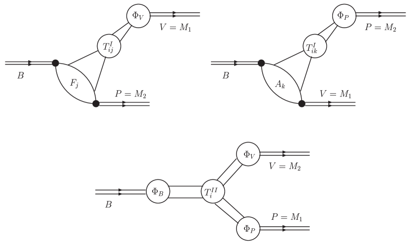
Figure 1: Graphical representation of the QCD factorization formula.

where $\phi_{M_{i}}$ with $M_{i}=V,P,B$ are the leading twist light cone distribution amplitudes (LCDA) of the valence quark Fock states. The light cone momentum fractions of the constituent quarks of the vector, pseudo-scalar and $B$ mesons are given respectively by $x,y,$ and $\xi$. The form factors for $B\to P$ and $B\to V$ semi-leptonic decays, evaluated at $k^{2}=0$, are denoted by $F_{j}^{B\rightarrow P}(0)$ and $A_{k}^{B\rightarrow V}(0)$. The hadronic decay amplitude involves both soft and hard contributions. At leading order, all the non-perturbative effects are assumed to be contained in the semi-leptonic form factors and the light cone distribution amplitudes. Then, non-factorizable interactions are dominated by hard gluon exchanges (in the case where the $O(\Lambda_{QCD}/m_{b}$) terms are neglected) and can be calculated perturbatively, in order to correct the naive factorization approximation. These hard scattering kernels, $T_{ik}^{I}$ and $T_{i}^{II}$, are calculable order by order in perturbation theory. The naive factorization terms are recovered by the leading terms of $T_{ik}^{I}$ and $T_{ij}^{I}$ coming from the tree level, whereas vertex and penguin corrections (Fig. 1) are included at the order of $\alpha_{s}$ in $T_{ik}^{I}$ and $T_{ij}^{I}$. The hard interactions (at order $O(\alpha_{s}$)) between the spectator quark and the emitted meson (Fig. 1), at large gluon momentum, are taken into account by $T_{i}^{II}$.

The coefficients, $a_{i}^{p}(M_{1}M_{2})$, written as a linear combination of Wilson coefficients, $C_{i}(\mu)$, (see Table 1) are calculated at next-to-leading order in $\alpha_{s}$ and contain all the non-factorizable effects. Their general form is [50],

$$a_{i}^{p}(M_{1}M_{2})=\left(C_{i}+\frac{C_{i\pm 1}}{N_{c}}\right)N_{i}(M_{2})\\ +\,\frac{C_{i\pm 1}}{N_{c}}\,\frac{C_{F}\alpha_{s}}{4\pi}\left[V_{i}(M_{2})+\frac{4\pi^{2}}{N_{c}}\,H_{i}(M_{1}M_{2})\right]+P_{i}^{p}(M_{2})\,,$$ (20)

where $p$ denotes the $u$ or $c$ quark. $N_{i}(M_{2})=0$ if $i=6,8$ with $M_{2}=V$, and $N_{i}(M_{2})=1$ for all other cases. The first terms in Eq. (20) include naive factorization followed by the vertex and the hard spectator interactions, whereas the last term describes the penguin corrections. Contrary to naive factorization, the QCDF approach takes into account the flavour of the final state through the coefficients, $a_{i}^{p}(M_{1}M_{2})$.

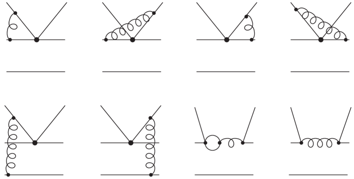
Figure 2: Vertex corrections, (first row) and hard spectator scattering and penguin corrections (second row) at the order $\alpha_{s}$.

The vertex corrections, $V_{i}(M_{2})$, (see Fig. 2) are given by [50],

$$V_{i}(M_{2})=\left\{\,\,\begin{array}[]{ll}{\displaystyle\int_{0}^{1}\!dx\,\Phi_{M_{2}}(x)\,\Big{[}12\ln\frac{m_{b}}{\mu}-18+g(x)\Big{]}}\,;&\qquad i=\mbox{1--4},9,10,\\[11.38092pt] {\displaystyle\int_{0}^{1}\!dx\,\Phi_{M_{2}}(x)\,\Big{[}-12\ln\frac{m_{b}}{\mu}+6-g(1-x)\Big{]}}\,;&\qquad i=5,7,\\[11.38092pt] {\displaystyle\int_{0}^{1}\!dx\,\Phi_{m_{2}}(x)\,\Big{[}-6+h(x)\Big{]}}\,;&\qquad i=6,8,\end{array}\right.$$ (21)

where, $\Phi_{M_{2}}(x)$, is the light-cone amplitude for a pseudo-scalar or vector meson and, $\Phi_{m_{2}}(x)$, is the twist-3 amplitude for the same mesons. The kernels $g(x)$ and $h(x)$ have the following form [50],

$$g(x) =3\left(\frac{1-2x}{1-x}\ln x-i\pi\right)$$ (22)

$$\quad\mbox{}+\left[2\,\mbox{Li}_{2}(x)-\ln^{2}\!x+\frac{2\ln x}{1-x}-(3+2i\pi)\ln x-(x\leftrightarrow 1-x)\right],$$

$$h(x) =2\,\mbox{Li}_{2}(x)-\ln^{2}\!x-(1+2\pi i)\,\ln x-(x\leftrightarrow 1-x)\,.$$

Next, $H_{i}(M_{1}M_{2})$ (see Fig. 2) describes the hard gluon exchanges between the spectator quark in the $B$ meson and the emitted meson, $M_{i}$ (pseudo-scalar or vector). These hard scattering corrections include chirally-enhanced contributions and take the form [50],

$$H_{i}(M_{1}M_{2})=\left\{\,\,\begin{array}[]{ll}{\displaystyle\frac{m_{B}}{\lambda_{B}}\int_{0}^{1}\!dx\int_{0}^{1}\!dy\left[\frac{\Phi_{M_{2}}(x)\Phi_{M_{1}}(y)}{\bar{x}\bar{y}}+r_{\chi}^{M_{1}}\,\frac{\Phi_{M_{2}}(x)\Phi_{m_{1}}(y)}{x\bar{y}}\right]}\,;&\\ {\displaystyle-\frac{m_{B}}{\lambda_{B}}\int_{0}^{1}\!dx\int_{0}^{1}\!dy\left[\frac{\Phi_{M_{2}}(x)\Phi_{M_{1}}(y)}{x\bar{y}}+r_{\chi}^{M_{1}}\,\frac{\Phi_{M_{2}}(x)\Phi_{m_{1}}(y)}{\bar{x}\bar{y}}\right]}\,;&\\ {\displaystyle\!\!0}\,;&\end{array}\right.$$

with $\frac{m_{B}}{\lambda_{B}}=\int_{0}^{1}d\xi\frac{\phi_{B}(\xi)}{\xi}$ and where the subscript $i$ goes as in Eq. (21). $H_{i}(M_{1}M_{2})$ is multiplied by $B_{M_{1}M_{2}}/A_{M_{1}M_{2}}$ given by:

$$\frac{B_{M_{1}M_{2}}}{A_{M_{1}M_{2}}}=\left\{\,\,\begin{array}[]{ll}{\displaystyle\frac{f_{B}f_{M_{1}}}{m_{B}^{2}F_{1}^{B\to M_{1}}(0)\,}}\,;&\qquad\mbox{if~{}}M_{1}=M_{2}=P,\\ {\displaystyle\frac{f_{B}f_{M_{1}}}{m_{B}^{2}A_{0}^{B\to M_{1}}(0)\,}}\,;&\qquad\mbox{if~{}}M_{1}=V,\,M_{2}=P,\\ {\displaystyle\frac{f_{B}f_{M_{1}}}{m_{B}^{2}F_{1}^{B\to M_{1}}(0)\,}}\,;&\qquad\mbox{if~{}}M_{1}=P,\,M_{2}=V,\end{array}\right.$$ (23)

with the usual definitions for $f_{B},f_{M_{i}},A_{0}^{B\rightarrow V}(0),F_{1}^{B\to P}(0)$ and $m_{B}$. The chiral enhancement factor is parameterized by the term $r_{\chi}^{M_{1}}=2m_{M_{1}}^{2}/m_{b}(\mu)(m_{1}+m_{2})(\mu)$, with $m_{1}$ and $m_{2}$ being the current quark masses of the valence quarks in the meson.

Finally, $P_{i}^{p}(M_{2})$ are the QCD penguin ($i=4,6$) and electroweak penguin ($i=8,10$) contributions. These quantities contain all of the non-perturbative dynamics and are the result of the convolution of hard scattering kernels, $G_{M_{2}}(s,x)$, with meson distribution amplitudes, $\Phi_{M_{i}}(x)$, such as,

$$G_{M_{2}}(s) =\int_{0}^{1}\!dx\,G(s-i\epsilon,1-x)\,\Phi_{M_{2}}(x)\ ,$$

$$\hat{G}_{M_{2}}(s) =\int_{0}^{1}\!dx\,G(s-i\epsilon,1-x)\,\Phi_{m_{2}}(x)\,.$$ (24)

The function $G(s,x)$ is given in Ref. [50]. The imaginary parts arising in the previous penguin functions, $g(x)$, $h(x)$, and $G(s,x)$, give us three sources of strong re-scattering phases. If $M_{2}$ is a pseudo-scalar, the penguin contributions, $P_{i}^{p}(M_{2})$, for $i=4,6,8,10$, are respectively [50]:

$$P_{i}^{p}(M_{2})=\left\{\,\,\begin{array}[]{l}\frac{C_{F}\alpha_{s}}{4\pi N_{c}}\,\Bigg{\{}C_{1}\!\left[\frac{4}{3}\ln\frac{m_{b}}{\mu}+\frac{2}{3}-G_{M_{2}}(s_{p})\right]\!+C_{3}\!\left[\frac{8}{3}\ln\frac{m_{b}}{\mu}+\frac{4}{3}-G_{M_{2}}(0)-G_{M_{2}}(1)\right]\\ +(C_{4}+C_{6})\!\left[\frac{4n_{f}}{3}\ln\frac{m_{b}}{\mu}-(n_{f}-2)\,G_{M_{2}}(0)-G_{M_{2}}(s_{c})-G_{M_{2}}(1)\right]\\ -2C_{8g}^{\rm eff}\int_{0}^{1}\frac{dx}{1-x}\,\Phi_{M_{2}}(x)\Bigg{\}}\,;\\[11.38092pt] \frac{C_{F}\alpha_{s}}{4\pi N_{c}}\,\Bigg{\{}C_{1}\!\left[\frac{4}{3}\ln\frac{m_{b}}{\mu}+\frac{2}{3}-\hat{G}_{M_{2}}(s_{p})\right]\!+C_{3}\!\left[\frac{8}{3}\ln\frac{m_{b}}{\mu}+\frac{4}{3}-\hat{G}_{M_{2}}(0)-\hat{G}_{M_{2}}(1)\right]\\ +(C_{4}+C_{6})\!\left[\frac{4n_{f}}{3}\ln\frac{m_{b}}{\mu}-(n_{f}-2)\,\hat{G}_{M_{2}}(0)-\hat{G}_{M_{2}}(s_{c})-\hat{G}_{M_{2}}(1)\right]\\ -2C_{8g}^{\rm eff}\Bigg{\}}\,;\\[11.38092pt] \frac{\alpha}{9\pi N_{c}}\,\Bigg{\{}(C_{1}+N_{c}C_{2})\left[\frac{4}{3}\ln\frac{m_{b}}{\mu}+\frac{2}{3}-\hat{G}_{M_{2}}(s_{p})\right]-3C_{7\gamma}^{\rm eff}\Bigg{\}}\,;\\[11.38092pt] \frac{\alpha}{9\pi N_{c}}\,\Bigg{\{}(C_{1}+N_{c}C_{2})\left[\frac{4}{3}\ln\frac{m_{b}}{\mu}+\frac{2}{3}-G_{M_{2}}(s_{p})\right]-3C_{7\gamma}^{\rm eff}\int_{0}^{1}\frac{dx}{1-x}\,\Phi_{M_{2}}(x)\Bigg{\}}\,;\end{array}\right.$$

$s_{q}=m_{q}^{2}/m_{b}^{2}$ is the mass ratio and can be equal to $s_{u}=s_{d}=0,s_{c}=m_{c}^{2}/m_{b}^{2}$ or $s_{b}=1$. All active quarks at the scale $\mu=O(m_{b})$ are represented by $q^{\prime}=u,d,s,c,b$. The other parameters are $C_{i}\equiv C_{i}(\mu)$ (in Naive Dimensional Regularization), $\alpha_{s}\equiv\alpha_{s}(\mu)$ (next to leading order), $C_{F}=(N_{c}^{2}-1)/2N_{c}$ with $N_{c}=3$. If $M_{2}$ is a vector meson, $P_{i}^{p}(M_{2})$ for $i=4,6,8,10$, respectively, take the form [50]:

$$P_{i}^{p}(M_{2})=\left\{\,\,\begin{array}[]{l}\frac{C_{F}\alpha_{s}}{4\pi N_{c}}\,\Bigg{\{}C_{1}\!\left[\frac{4}{3}\ln\frac{m_{b}}{\mu}+\frac{2}{3}-G_{M_{2}}(s_{p})\right]\!+C_{3}\!\left[\frac{8}{3}\ln\frac{m_{b}}{\mu}+\frac{4}{3}-G_{M_{2}}(0)-G_{M_{2}}(1)\right]\\ +(C_{4}+C_{6})\!\left[\frac{4n_{f}}{3}\ln\frac{m_{b}}{\mu}-(n_{f}-2)\,G_{M_{2}}(0)-G_{M_{2}}(s_{c})-G_{M_{2}}(1)\right]\\ -2C_{8g}^{\rm eff}\int_{0}^{1}\frac{dx}{1-x}\,\Phi_{M_{2}}(x)\Bigg{\}}\,;\\[11.38092pt] -\frac{C_{F}\alpha_{s}}{4\pi N_{c}}\,\Bigg{\{}C_{1}\,\hat{G}_{M_{2}}(s_{p})+C_{3}\,\Big{[}\hat{G}_{M_{2}}(0)+\hat{G}_{M_{2}}(1)\Big{]}\\ (C_{4}+C_{6})\left[(n_{f}-2)\,\hat{G}_{M_{2}}(0)+\hat{G}_{M_{2}}(s_{c})+\hat{G}_{M_{2}}(1)\right]\Bigg{\}}\,;\\[11.38092pt] -\frac{\alpha}{9\pi N_{c}}\,\Bigg{\{}(C_{1}+N_{c}C_{2})\,\hat{G}_{M_{2}}(s_{p})\Bigg{\}}\,;\\[11.38092pt] \frac{\alpha}{9\pi N_{c}}\,\Bigg{\{}(C_{1}+N_{c}C_{2})\left[\frac{4}{3}\ln\frac{m_{b}}{\mu}+\frac{2}{3}-G_{M_{2}}(s_{p})\right]-3C_{7\gamma}^{\rm eff}\int_{0}^{1}\frac{dx}{1-x}\,\Phi_{M_{2}}(x)\Bigg{\}}\,.\end{array}\right.$$

The vertex and penguin corrections to the hard-scattering kernels are evaluated at the scale $\mu\sim m_{b}$. Because the gluon is off-shell, the strong coupling constant, $\alpha_{s}(\mu)$, the Wilson coefficients, $C_{i}(\mu)$, and then the hard-scattering contributions, $P_{i}^{p}(M_{2})$, are evaluated at the scale $\mu_{h}=\sqrt{\Lambda_{h}\mu}$, with $\Lambda_{h}=0.5$ GeV, rather than the scale $\mu=m_{b}$.

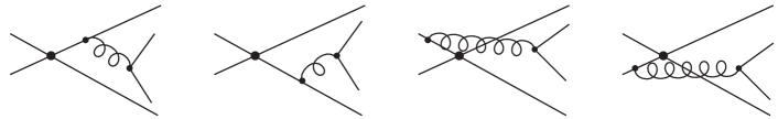
Figure 3: Order $\alpha_{s}$ corrections to the weak annihilation.

It has been shown in Ref. [24, 51] that the weak annihilation contributions cannot be neglected in $B$ meson decays even though they are power suppressed in heavy-quark limit ($\Lambda_{QCD}/m_{b}$). Moreover, their contributions could carry large strong phases with QCD corrections and hence, large $CP$ violation might be obtained in $B$ meson decays. The annihilation contributions, at leading order in $\alpha_{s}$, are given by the diagrams drawn in Fig. 3. They do not arise in the QCD factorization formulation because of their endpoint singularities. Nevertheless, their contributions denoted by $A_{k}^{i}(M_{1}M_{2})$ ($\equiv A_{k}^{i}$ for simplicity), are approximated in terms of convolutions of hard scattering kernels with light cone expansions for the final state mesons. If we define $x$ as the longitudinal momentum fraction of the quark contained in $M_{2}$ and ${\bar{y}}=1-y$, the momentum fraction of the antiquark contained in $M_{1}$, then the diagrams related to the annihilation contributions can be expressed as [50]:

$$A_{1}^{i}\!\! = \!\!\pi\alpha_{s}\int_{0}^{1}\!dxdy\,\left\{\Phi_{M_{2}}(x)\,\Phi_{M_{1}}(y)\left[\frac{1}{y(1-x\bar{y})}+\frac{1}{\bar{x}^{2}y}\right]+r_{\chi}^{M_{1}}r_{\chi}^{M_{2}}\,\Phi_{m_{2}}(x)\,\Phi_{m_{1}}(y)\,\frac{2}{\bar{x}y}\right\},$$

$$A_{2}^{i}\!\! = \!\!\pi\alpha_{s}\int_{0}^{1}\!dxdy\,\left\{\Phi_{M_{2}}(x)\,\Phi_{M_{1}}(y)\left[\frac{1}{\bar{x}(1-x\bar{y})}+\frac{1}{\bar{x}y^{2}}\right]+r_{\chi}^{M_{1}}r_{\chi}^{M_{2}}\,\Phi_{m_{2}}(x)\,\Phi_{m_{1}}(y)\,\frac{2}{\bar{x}y}\right\},$$

$$A_{3}^{i}\!\! = \!\!\pi\alpha_{s}\int_{0}^{1}\!dxdy\,\left\{r_{\chi}^{M_{1}}\,\Phi_{M_{2}}(x)\,\Phi_{m_{1}}(y)\,\frac{2\bar{y}}{\bar{x}y(1-x\bar{y})}-r_{\chi}^{M_{2}}\,\Phi_{M_{1}}(y)\,\Phi_{m_{2}}(x)\,\frac{2x}{\bar{x}y(1-x\bar{y})}\right\},$$

and,

$$A_{1}^{f}\!\! = \!\!A_{2}^{f}=0\,,$$

$$A_{3}^{f}\!\! = \!\!\pi\alpha_{s}\int_{0}^{1}\!dxdy\,\left\{r_{\chi}^{M_{1}}\,\Phi_{M_{2}}(x)\,\Phi_{m_{1}}(y)\,\frac{2(1+\bar{x})}{\bar{x}^{2}y}+r_{\chi}^{M_{2}}\,\Phi_{M_{1}}(y)\,\Phi_{m_{2}}(x)\,\frac{2(1+y)}{\bar{x}y^{2}}\right\},$$

where the superscripts ‘$i$’ and ‘$f$’ refer to gluon emission from the initial and final-state quarks, respectively. When $M_{1}$ is a vector meson and $M_{2}$ a pseudo-scalar, (i.e. in the case of decays such as $B\to M_{1}^{V}M_{2}^{PS}$) one has to change the sign of the second (twist-4) term in $A_{1}^{i}$, the first (twist-2) term in $A_{2}^{i}$, and the second term in $A_{3}^{i}$ and $A_{3}^{f}$. When $M_{2}$ is a vector meson and $M_{1}$ a pseudo-scalar (i.e. in the case of decays such as $B\to M_{1}^{PS}M_{2}^{V}$), one only has to change the overall sign of $A_{2}^{i}$.

Taking into account the flavour structure of the various operators involved in the weak annihilation topologies, the annihilation amplitude can be written as,

$$A^{a}(B\to M_{1}M_{2})\propto f_{B}f_{M_{1}}f_{M_{2}}\sum_{p=u,c}\sum_{i=1,4}V_{pb}V_{ps}^{*}b_{i}\ .$$ (25)

The coefficients $b_{i}$ in Eq. (25) are expressed in terms of linear combinations of $A_{i}(M_{1}M_{2})$ and they take the following form:

$$b_{1} =\frac{C_{F}}{N_{c}^{2}}C_{1}A_{1}^{i}\ ,$$

$$b_{2} =\frac{C_{F}}{N_{c}^{2}}C_{2}A_{1}^{i}\ ,$$

$$b_{3} =\frac{C_{F}}{N_{c}^{2}}\Biggl{\{}C_{3}A_{1}^{i}+C_{5}A_{3}^{i}+\Big{[}C_{5}+N_{c}C_{6}\Big{]}A_{3}^{f}\Biggr{\}}\ ,$$

$$b_{4} =\frac{C_{F}}{N_{c}^{2}}\Big{\{}C_{4}A_{1}^{i}+C_{6}A_{2}^{i}\Big{\}}\ ,$$

$$b_{3}^{ew} =\frac{C_{F}}{N_{c}^{2}}\Biggl{\{}C_{9}A_{1}^{i}+C_{7}A_{3}^{i}+\Big{[}C_{7}+N_{c}C_{8}\Big{]}A_{3}^{f}\Biggr{\}}\ ,$$

$$b_{4}^{ew} =\frac{C_{F}}{N_{c}^{2}}\Big{\{}C_{10}A_{1}^{i}+C_{8}A_{2}^{i}\Big{\}}\ ,$$ (26)

where $b_{i}(\equiv b_{i}(M_{1},M_{2}))$ are respectively the current-current annihilation parameters arising from the hadronic matrix elements of the effective operators for $i=1,2$, the QCD penguin annihilation parameters for $i=3,4$ and the electroweak penguin annihilation parameters for $i=3,4$ with the subscript $ew$ attached to $b_{i}$. The quantities $b_{i}$ depend on the final state mesons through the terms $A_{k}^{i}$ defined previously.

The calculation of the hard spectator as well as the annihilation contributions involves the twist-3 distribution amplitude, $\phi_{m_{i}}$. It happens that these power-suppressed contributions involve divergences because of the non-vanishing endpoint behaviour of $\phi_{m_{i}}$. This divergence, $X^{M_{i}}$, analyzed as (for example),

$$\int_{0}^{1}\frac{dy}{\bar{y}}\,\Phi_{m_{i}}(y) = \Phi_{m_{i}}(1)\,\int_{0}^{1}\frac{dy}{\bar{y}}+\int_{0}^{1}\frac{dy}{\bar{y}}\,\Big{[}\Phi_{m_{i}}(y)-\Phi_{m_{i}}(1)\Big{]}\ ,$$ (27)

$$\equiv \Phi_{m_{i}}(1)\,X^{M_{i}}+\int_{0}^{1}\frac{dy}{[\bar{y}]_{+}}\,\Phi_{m_{i}}(y)\,,$$

is applied in the following cases as well:

$$\int_{0}^{1}\frac{dy}{y}\to X^{M_{i}}\,,\qquad{\rm and}\;\;\int_{0}^{1}\!dy\,\frac{\ln y}{y}\to-\frac{1}{2}\,(X^{M_{i}})^{2}\,.$$ (28)

The perturbative calculation of the hard scattering spectator and annihilation contributions is regulated by a physical scale of order $\Lambda_{QCD}$. Therefore, treating the divergent endpoint parameterized by $X^{M_{i}}$ in a phenomenological way, one may take the following ansatz:

$$X^{M_{i}}=\left(1+\varrho^{M_{i}}\,e^{i\varphi^{M_{i}}}\right)\ln\frac{m_{B}}{\Lambda_{h}}\,,\qquad{\rm with}\;\;\qquad\Lambda_{h}=0.5\,\mbox{GeV}\,,$$ (29)

where the phase $\varphi^{M_{i}}$ and the coefficient $\varrho^{M_{i}}$ give rise to a dynamically generated strong interaction phase. This divergence, $X^{M_{i}}$, coming from the twist-3 contribution holds for both hard spectator scattering, $X_{H}^{M_{i}}$, and weak annihilation, $X_{A}^{M_{i}}$. It is expected to take the form given in Eq. (29) since the soft interaction is regulated by a physical scale $\Lambda_{QCD}/m_{b}$. Moreover a strong phase (complex part of Eq. (29)) can arise because of multiple soft scattering. In this model dependent way of dealing with the two latter corrections, we assume that $X_{H}^{M_{i}}$ and $X_{A}^{M_{i}}$ are not universal. In other words, they depend on the flavour of the meson, $M_{i}$, but they do not depend on the weak vertex. Moreover, in order to make this dependence more efficient, in all the calculations we use the full distribution amplitudes for $\phi_{M_{i}}$ and $\phi_{m_{i}}$ by taking into account the Gegenbauer expansion of the asymptotic distribution amplitude.

4 Mixing scheme

4.1 $\boldsymbol{\rho^{0}-\omega}$ mixing scheme

The direct $CP$ violating asymmetry parameter, $a_{CP}$, is found to be small for most of the non-leptonic exclusive $B$ decays when either the naive or QCD factorization framework is applied. However, in the case of $B$ decay channels involving the $\rho^{0}$ meson, it appears that the asymmetry may be large in the vicinity of $\omega$ meson mass. To obtain a large signal for direct $CP$ violation requires some mechanism to make both $\sin\delta$ and $r$ large (see Eq. (42) below). We stress that $\rho^{0}-\omega$ mixing has the dual advantages that the strong phase difference is large (passing rapidly through $90^{o}$ at the $\omega$ resonance) and well known [28, 29, 30, 31, 52, 53]. In the vector meson dominance model [54], the photon propagator is dressed by coupling to the vector mesons $\rho^{0}$ and $\omega$. In this regard, the $\rho^{0}-\omega$ mixing mechanism [55, 56, 57] has been developed. Let $A$ be the amplitude for the decay $B\rightarrow\rho^{0}(\omega)M_{1}\;\rightarrow\pi^{+}\pi^{-}\;M_{1}$, then one has,

$$A=\langle M_{1}\;\pi^{-}\pi^{+}|H^{T}|B\rangle+\langle M_{1}\;\pi^{-}\pi^{+}|H^{P}|B\rangle\ ,$$ (30)

with $H^{T}$ and $H^{P}$ being the Hamiltonians for the tree and penguin operators. Here $M_{1}$ denotes a pseudo-scalar meson. We can define the relative magnitude and phases between these two contributions as follows,

$$A =\langle M_{1}\;\pi^{-}\pi^{+}|H^{T}|B\rangle[1+re^{i\delta}e^{i\phi}]\ ,$$

$$\bar{A} =\langle\overline{M_{1}}\;\pi^{+}\pi^{-}|H^{T}|\bar{B}\rangle[1+re^{i\delta}e^{-i\phi}]\ ,$$ (31)

where $\delta$ and $\phi$ are strong and weak phases, respectively. The phase $\phi$ arises from the appropriate combination of CKM matrix elements. In case of $b\to d$ or $b\to s$ transitions, $\phi$ is given by $\phi={\rm arg}[(V_{tb}V_{td}^{\star})/(V_{ub}V_{ud}^{\star})]$ or ${\rm arg}[(V_{tb}V_{ts}^{\star})/(V_{ub}V_{us}^{\star})]$, respectively. As a result, $\sin\phi$ is equal to $\sin\alpha\;(\sin\gamma)$ for $b\to d\;(b\to s)$, with $\alpha\;(\gamma)$ defined in the standard way [59]. $\sin\phi\;(\cos\phi)$ therefore takes the following form in case of a $b\to d$ transition,

$$\sin\phi =\frac{\eta}{\sqrt{\left(\rho-(\rho^{2}+\eta^{2})(1-\frac{\lambda^{2}}{2})\right)^{2}+\eta^{2}}}\ ,$$

$$\cos\phi =\frac{\rho-(\rho^{2}+\eta^{2})(1-\frac{\lambda^{2}}{2})}{\sqrt{\left(\rho-(\rho^{2}+\eta^{2})(1-\frac{\lambda^{2}}{2})\right)^{2}+\eta^{2}}}\ ,$$ (32)

and in case of a $b\to s$ transition,

$$\sin\phi =\frac{-\eta(1-\frac{\lambda^{2}}{2})}{\sqrt{\left(-\lambda^{2}(\rho^{2}+\eta^{2})-\rho(1-\frac{\lambda^{2}}{2})\right)^{2}+\left(\eta^{2}(1-\frac{\lambda^{2}}{2})\right)^{2}}}\ ,$$

$$\cos\phi =\frac{-\lambda^{2}(\rho^{2}+\eta^{2})-\rho(1-\frac{\lambda^{2}}{2})}{\sqrt{\left(-\lambda^{2}(\rho^{2}+\eta^{2})-\rho(1-\frac{\lambda^{2}}{2})\right)^{2}+\left(\eta^{2}(1-\frac{\lambda^{2}}{2})\right)^{2}}}\ .$$ (33)

Regarding the parameter, $r$, it represents the absolute value of the ratio of tree and penguin amplitudes:

$$r\equiv\left|\frac{\langle\rho^{0}(\omega)M_{1}|H^{P}|B\rangle}{\langle\rho^{0}(\omega)M_{1}|H^{T}|B\rangle}\right|.$$ (34)

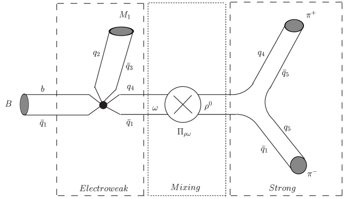
Figure 4: Inclusion of the $\rho-\omega$ mixing in $B\to\rho^{0}M_{1}$ decay.

With this mechanism (see Fig. 4), to first order in isospin violation, we have the following results when the invariant mass of $\pi^{+}\pi^{-}$ is near the $\omega$ resonance mass,

$$\langle M_{1}\pi^{-}\pi^{+}|H^{T}|B\rangle =\frac{g_{\rho}}{s_{\rho}s_{\omega}}\tilde{\Pi}_{\rho\omega}(t_{\omega}+t_{\omega}^{a})+\frac{g_{\rho}}{s_{\rho}}(t_{\rho}+t_{\rho}^{a})\ ,$$

$$\langle M_{1}\pi^{-}\pi^{+}|H^{P}|B\rangle =\frac{g_{\rho}}{s_{\rho}s_{\omega}}\tilde{\Pi}_{\rho\omega}(p_{\omega}+p_{\omega}^{a})+\frac{g_{\rho}}{s_{\rho}}(p_{\rho}+p_{\rho}^{a})\ .$$ (35)

Here $t_{V}^{(a)}\;(V=\rho\;{\rm or}\;\omega)$ is the tree (tree annihilation) amplitude and $p_{V}^{(a)}$ the penguin (penguin annihilation) amplitude for producing a vector meson, $V$, $g_{\rho}$ is the coupling for $\rho^{0}\rightarrow\pi^{+}\pi^{-}$, $\tilde{\Pi}_{\rho\omega}$ is the effective $\rho-\omega$ mixing amplitude, and $s_{V}$ is from the inverse propagator of the vector meson $V$, $s_{V}=s-m_{V}^{2}+im_{V}\Gamma_{V}$ (with $\sqrt{s}$ the invariant mass of the $\pi^{+}\pi^{-}$ pair). We stress that the direct coupling $\omega\rightarrow\pi^{+}\pi^{-}$ is effectively absorbed into $\tilde{\Pi}_{\rho\omega}$ [60, 61, 62, 63, 64], leading to the explicit $s$ dependence of $\tilde{\Pi}_{\rho\omega}$. Making the expansion $\tilde{\Pi}_{\rho\omega}(s)=\tilde{\Pi}_{\rho\omega}(m_{\omega}^{2})+(s-m_{w}^{2})\tilde{\Pi}_{\rho\omega}^{\prime}(m_{\omega}^{2})$, the $\rho^{0}-\omega$ mixing parameters were determined in the fit of Gardner and O’Connell [65]: $\Re e\;\tilde{\Pi}_{\rho\omega}(m_{\omega}^{2})=-3500\pm 300\;{\rm MeV}^{2},\;\;\;\Im m\;\tilde{\Pi}_{\rho\omega}(m_{\omega}^{2})=-300\pm 300\;{\rm MeV}^{2}$, and $\tilde{\Pi}_{\rho\omega}^{\prime}(m_{\omega}^{2})=0.03\pm 0.04$. In practice, the effect of the derivative term is negligible. From Eqs. (4.1, 4.1) one has,

$$re^{i\delta}e^{i\phi}=\frac{\tilde{\Pi}_{\rho\omega}(p_{\omega}+p_{\omega}^{a})+s_{\omega}(p_{\rho}+p_{\rho}^{a})}{\tilde{\Pi}_{\rho\omega}(t_{\omega}+t_{\omega}^{a})+s_{\omega}(t_{\rho}+t_{\rho}^{a})}\ .$$ (36)

Defining

$$\frac{p_{\omega}+p_{\omega}^{a}}{t_{\rho}+t_{\rho}^{a}}\equiv r^{\prime}e^{i(\delta_{q}+\phi)}\ ,\;\;\;\;\frac{t_{\omega}+t_{\omega}^{a}}{t_{\rho}+t_{\rho}^{a}}\equiv\alpha e^{i\delta_{\alpha}}\ ,\;\;\;\;\frac{p_{\rho}+p_{\rho}^{a}}{p_{\omega}+p_{\omega}^{a}}\equiv\beta e^{i\delta_{\beta}}\ ,$$ (37)

where $\delta_{\alpha},\delta_{\beta}$ and $\delta_{q}$ are strong relative phases (absorptive part). Substituting Eq. (37) into Eq. (36) one finds:

$$re^{i\delta}=r^{\prime}e^{i\delta_{q}}\frac{\tilde{\Pi}_{\rho\omega}+\beta e^{i\delta_{\beta}}s_{\omega}}{s_{\omega}+\tilde{\Pi}_{\rho\omega}\alpha e^{i\delta_{\alpha}}}\ .$$ (38)

Defining $\alpha e^{i\delta_{\alpha}}=f+gi,\;\;\;\beta e^{i\delta_{\beta}}=b+ci$ and $r^{\prime}e^{i\delta_{q}}=d+ei$, Eq. (38) becomes,

$$re^{i\delta}=\frac{C+iD}{(s-m_{\omega}^{2}+f\Re e\;\tilde{\Pi}_{\rho\omega}-g\Im m\;\tilde{\Pi}_{\rho\omega})^{2}+(f\Im m\;\tilde{\Pi}_{\rho\omega}+g\Re e\;\tilde{\Pi}_{\rho\omega}m_{\omega}\Gamma_{\omega})^{2}}\ ,$$ (39)

where $C$ and $D$ are given by:

$$C=\bigl{(}s-m_{\omega}^{2}+f\Re e\;\tilde{\Pi}_{\rho\omega}-g\Im m\;\tilde{\Pi}_{\rho\omega}\bigr{)}\Biggl{\{}d\biggl{[}\Re e\;\tilde{\Pi}_{\rho\omega}+b(s-m_{\omega}^{2})-cm_{\omega}\Gamma_{\omega}\biggr{]}\\ -e\biggl{[}\Im m\;\tilde{\Pi}_{\rho\omega}+bm_{\omega}\Gamma_{\omega}+c(s-m_{\omega}^{2})\biggr{]}\Biggr{\}}\\ +\bigl{(}f\Im m\;\tilde{\Pi}_{\rho\omega}+m_{\omega}\Gamma_{\omega}+g\Re e\;\tilde{\Pi}_{\rho\omega}\bigr{)}\Biggl{\{}e\biggl{[}\Re e\;\tilde{\Pi}_{\rho\omega}+b(s-m_{\omega}^{2})-cm_{\omega}\Gamma_{\omega}\biggr{]}\\ +d\biggl{[}\Im m\;\tilde{\Pi}_{\rho\omega}+bm_{\omega}\Gamma_{\omega}+c(s-m_{\omega}^{2})\biggr{]}\Biggr{\}}\ ,$$ (40)

and

$$D=\bigl{(}s-m_{\omega}^{2}+f\Re e\;\tilde{\Pi}_{\rho\omega}-g\Im m\;\tilde{\Pi}_{\rho\omega}\bigr{)}\Biggl{\{}e\biggl{[}\Re e\;\tilde{\Pi}_{\rho\omega}+d(s-m_{\omega}^{2})-cm_{\omega}\Gamma_{\omega}\biggr{]}\\ +d\biggl{[}\Im m\;\tilde{\Pi}_{\rho\omega}+bm_{\omega}\Gamma_{\omega}+c(s-m_{\omega}^{2})\biggr{]}\Biggr{\}}\\ -\bigl{(}f\Im m\;\tilde{\Pi}_{\rho\omega}+m_{\omega}\Gamma_{\omega}+g\Re e\;\tilde{\Pi}_{\rho\omega}\bigr{)}\Biggl{\{}d\biggl{[}\Re e\;\tilde{\Pi}_{\rho\omega}+b(s-m_{\omega}^{2})-cm_{\omega}\Gamma_{\omega}\biggr{]}\\ -e\biggl{[}\Im m\;\tilde{\Pi}_{\rho\omega}+bm_{\omega}\Gamma_{\omega}+c(s-m_{\omega}^{2})\biggr{]}\Biggr{\}}\ .$$ (41)

Knowing the ratio, $r$, and the strong phase, $\delta$, from Eq. (38) as well as the weak phase, $\phi$, from the CKM matrix, it is therefore possible to calculate the $CP$ violating asymmetry, $a_{CP}$, including the $\rho^{0}-\omega$ mixing mechanism:

$$a_{CP}\equiv\frac{|A|^{2}-|\bar{A}|^{2}}{|A|^{2}+|\bar{A}|^{2}}=\frac{-2r\sin\delta\sin\phi}{1+2r\cos\delta\cos\phi+r^{2}}\ .$$ (42)

4.2 $\boldsymbol{\eta-\eta^{\prime}}$ mixing scheme

The evaluation of the decay constants for the pseudo-scalar mesons $\eta$ and $\eta^{\prime}$ is not trivial. In this section, we recall briefly how the mixing $\eta-\eta^{\prime}$ is taken into account, see Ref. [66] for more details. The $\eta-\eta^{\prime}$ mixing scheme requires the assumption that their decay constants follow the pattern of particle state mixing. That is known as the Feldmann-Kroll-Stech (FKS) mixing scheme [67, 68], where the axial $U(1)$ anomaly is assumed to be the only effect that mixes the two flavor states $|\eta_{q}\rangle$ and $|\eta_{s}\rangle$. It is therefore possible to relate the two flavor states to the physical state by the following transformation,

$$\left(\begin{array}[]{c}|\eta\rangle\\ |\eta^{\prime}\rangle\end{array}\right)=\left(\begin{array}[]{cc}\cos\alpha&-\sin\alpha\\ \sin\alpha&\cos\alpha\\ \end{array}\right)\left(\begin{array}[]{c}|\eta_{q}\rangle\\ |\eta_{s}\rangle\\ \end{array}\right)\ ,$$ (43)

where $|\eta\rangle$ and $|\eta^{\prime}\rangle$ are the physical states and $\alpha$ the mixing angle in the flavor basis. Let us now define the matrix elements of the flavor diagonal axial-vector and pseudo-scalar densities in terms of decay constants, $f_{P}^{i}$ and $h_{P}^{i}$, where $i$ follows $q$ or $s$:

$$\langle P(q)|\bar{q}\gamma^{\mu}\gamma_{5}q|0\rangle=-\frac{i}{\sqrt{2}}f_{P}^{q}q^{\mu}\ ,$$

$$\langle P(q)|\bar{s}\gamma^{\mu}\gamma_{5}s|0\rangle=-if_{P}^{s}q^{\mu}\ ,$$

$$2m_{q}\langle P(q)|\bar{s}\gamma_{5}s|0\rangle=-\frac{i}{\sqrt{2}}h_{P}^{q}\ ,$$

$$2m_{s}\langle P(q)|\bar{s}\gamma_{5}s|0\rangle=-ih_{P}^{s}\ ,$$ (44)

where $q$ is $u$ or $d$. Assuming that the same angle, $\alpha$, applies to the decay constants defined previously, $f_{P}^{i}$ and $h_{P}^{i}$, this yields:

$$\left(\begin{array}[]{cc}f_{\eta}^{q}(h_{\eta}^{q})&f_{\eta}^{s}(h_{\eta}^{s})\\ f_{\eta^{\prime}}^{q}(h_{\eta^{\prime}}^{q})&f_{\eta^{\prime}}^{s}(h_{\eta^{\prime}}^{s})\\ \end{array}\right)=\left(\begin{array}[]{cc}\cos\alpha&-\sin\alpha\\ \sin\alpha&\cos\alpha\\ \end{array}\right)\left(\begin{array}[]{cc}f_{q}(h_{q})&0\\ 0&f_{s}(h_{s})\\ \end{array}\right)\ .$$ (45)

The anomaly matrix element, $a_{P}$, which is defined as

$$\langle P(q)|\frac{\alpha_{s}}{4\pi}G_{\mu\nu}^{A}\tilde{G}^{A,\mu\nu}|0\rangle=a_{P}\ ,$$ (46)

where $G_{\mu\nu}^{A}$ is the dual field strength tensor, can be related to the parameters, $f_{P}^{i}$ and $h_{i}^{q}$, through the following relation,

$$a_{P}=\frac{h_{P}^{q}-f^{q}_{P}m^{2}_{P}}{\sqrt{2}}=h_{P}^{s}-f_{P}^{s}m_{P}^{s}\ ,$$ (47)

by taking the divergence of the axial vector current $\bar{q}\gamma^{\mu}\gamma_{5}q$. Therefore, the parameters involved in the FKS scheme can be expressed in terms of three independent parameters, $f_{q}$, $f_{s}$ and the mixing angle $\alpha$. They have been determined from a fit to experimental data and their values are:

$$f_{q}=(1.07\pm 0.02)f_{\pi}\ ,\;\;f_{s}=(1.34\pm 0.06)f_{\pi}\ ,\;\;\;\alpha=39.3^{o}\pm 1.0^{o}\ .$$

5 CKM matrix

In most phenomenological applications, the widely used CKM matrix parametrization is the Wolfenstein parametrization [69, 70]. This has three main advantages in comparison with the standard parametrization [71, 72]: it allows us to make an explicit hierarchy, in terms of strength couplings, between quarks; it allows us easier analytical derivation and finally the four independent parameters, $\lambda,A,\rho$ and $\eta$, can be (in)directly measured experimentally. This parametrization can also be described in a geometrical representation, the so-called the unitarity triangle (UT), which offers another way to check effects of New Physics.

By expanding each element of the CKM matrix as a power series in the parameter $\lambda=\sin\theta_{c}=0.2224$ ($\theta_{c}$ is the Gell-Mann-Levy-Cabibbo angle), one gets (if $O(\lambda^{4})$ is neglected)

$${\hat{V}}_{CKM}=\left(\begin{array}[]{ccc}1-\frac{1}{2}\lambda^{2}&\lambda&A\lambda^{3}(\rho-i\eta)\\ -\lambda&1-\frac{1}{2}\lambda^{2}&A\lambda^{2}\\ A\lambda^{3}(1-\rho-i\eta)&-A\lambda^{2}&1\\ \end{array}\right)\ ,$$ (48)

where $\eta$ plays the well-known role of the $CP$-violating phase in the Standard Model framework. However, it may be more accurate to go beyond the leading order in terms of $\lambda$ in a perturbative expansion of the CKM matrix. It was found that the CKM matrix takes the following form (up to corrections of $O(\lambda^{7})$):

$${\hat{V}}_{CKM}=\left(\begin{array}[]{ccc}1-\frac{1}{2}\lambda^{2}-\frac{1}{8}\lambda^{4}&\lambda&A\lambda^{3}(\rho-i\eta)\\ -\lambda+\frac{1}{2}A^{2}\lambda^{5}(1-2(\rho+i\eta))&1-\frac{1}{2}\lambda^{2}-\frac{1}{8}\lambda^{4}(1+4A^{2})&A\lambda^{2}\\ A\lambda^{3}(1-\bar{\rho}-i\bar{\eta})&-A\lambda^{2}+\frac{1}{2}A\lambda^{4}(1-2(\rho+i\eta))&1-\frac{1}{2}A^{2}\lambda^{4}\\ \end{array}\right)\ ,$$ (49)

where

$$\bar{\rho}=\rho\biggl{(}1-\frac{\lambda^{2}}{2}\biggr{)}\;\;{\rm and}\;\;\bar{\eta}=\eta\biggl{(}1-\frac{\lambda^{2}}{2}\biggr{)}\ .$$ (50)

The corrections to the real and imaginary parts for the other terms can be safely neglected. In our phenomenological application, we will take into account the above corrections to $V_{ij}$ because some of them appear significant. Finally, due to the unitarity condition of the CKM matrix,

$${\hat{V}}_{CKM}^{\dagger}\cdot{\hat{V}}_{CKM}={\hat{I}}={\hat{V}}_{CKM}\cdot{\hat{V}}_{CKM}^{\dagger}\ ,$$ (51)

which ensures the absence of flavour-changing neutral-current (FCNC) processes at the tree level in the Standard Model, the most useful orthogonality relation in charmless $B$ decays is given by

$$V_{ud}V_{ub}^{*}+V_{cd}V_{cb}^{*}+V_{td}V_{tb}^{*}=0\ .$$ (52)

The CKM matrix, expressed in terms of the Wolfenstein parameters, is constrained with several experimental data. The main ones are the $b\to ul\bar{\nu}$ and $b\to cl\bar{\nu}$ decay processes, $s$ and $d$ mass oscillations, $\Delta m_{s},\Delta m_{d}$, and $CP$ violation in the kaon system ($\epsilon_{K}$). In our numerical applications we will take, in case of $68\%$ confidence level [9],

$$0.122<\rho<0.232\;\;{\rm and}\;\;0.334<\eta<0.414\ ,$$ (53)

and in case of $95\%$ confidence level [9],

$$0.076<\rho<0.380\;\;{\rm and}\;\;0.280<\eta<0.455\ .$$ (54)

The values for $A$ and $\lambda$ are assumed to be well determined experimentally [9]:

$$\lambda=0.2265\;\;{\rm and}\;\;A=0.801\ .$$ (55)

The angles $\alpha,\beta$ and $\gamma$ (to the Unitarity Triangle) corresponding to the values mentioned previously for $A,\lambda,\rho$ and $\eta$ are within the following limits (at $95\%$ confidence level):

$$70<\alpha<130\ ,\;\;20<\beta<30\ ,\;\;50<\gamma<70\ .$$ (56)

6 Input physical parameters

6.1 Quark masses

The running quark masses are used in order to calculate the matrix elements of penguin operators as well as the chiral enhancement factors. The quark mass is taken at the scale $\mu\simeq m_{b}$ in $B$ decays. Therefore one has [73] (in MeV),

$$m_{u}=m_{d}=3.7\ ,\;m_{s}=90\ ,\;m_{b}=4200\ ,\;m_{c}=1300\ ,$$ (57)

which corresponds to $m_{s}(\mu=1\;{\rm GeV})=140\;{\rm MeV}$. For meson masses, we shall use the following values [59] (in GeV):

$$m_{B^{\pm}} =5.279\ , m_{B^{0}} =5.279\ , m_{\eta} =0.515\ ,$$

$$m_{K^{\pm}} =0.493\ , m_{K^{0}} =0.497\ , m_{\eta^{{}^{\prime}}} =0.983\ ,$$

$$m_{\pi^{\pm}} =0.139\ , m_{\pi^{0}} =0.135\ , m_{\phi} =1.019\ ,$$

$$m_{\rho^{0}} =0.769\ , m_{\omega} =0.782\ , m_{K^{*}} =0.894\ .$$

6.2 Form factors and decay constants

The heavy(light)-to-light form factors, $F_{i}(k^{2})$ and $A_{j}(k^{2})$, depend on the inner structure of the hadrons. Here we shall primarily adopt the values of form factors for the pseudo-scalar to pseudo-scalar and pseudo-scalar to vector transitions obtained from QCD sum rule calculations. Moreover, we will keep the form factors $F_{i}^{B\to\pi}$ and $F_{i}^{B\to K}$ unconstrained, because of the large uncertainties entering into their calculation. In this way, the strong dependence of the branching ratios, for the decays $B\to X\pi$ and $B\to XK$, on the form factors $F_{i}^{B\to\pi}$ and $F_{i}^{B\to K}$ will be analyzed. For the others, their values are the following [66, 74, 75, 76]:

$$A_{j}^{B\to\rho} =0.37\ , A_{j}^{B\to\omega} =0.33\ ,$$

$$A_{j}^{B\to\phi} =0.0\ , A_{j}^{B\to K^{*}} =0.45\ .$$

For the special case of $F_{i}^{B\to\eta^{(^{\prime})}}$, the form factor is parameterized as follows [66]:

$$F_{i}^{B\to\eta^{(\prime)}}(0)=F_{1}\frac{f_{P}^{q}}{f_{\pi}}+F_{2}\frac{\sqrt{2}f_{P}^{q}+f_{P}^{s}}{\sqrt{3}f_{\pi}}\ ,$$ (58)

where $F_{1}$ behaves like $F_{i}^{B\to\pi}(0)$ in the FKS scheme and $F_{2}$ is taken to be around 0.1 [66].

The decay constants for pseudo-scalar, $f_{P}$, and vector, $f_{V}$, mesons do not suffer from uncertainties as large as those for form factors since they are well determined experimentally from leptonic and semi-leptonic decays. Let us first recall the usual definition for a pseudo-scalar,

$$\langle P(q)|\bar{q}_{1}\gamma_{\mu}\gamma_{5}q_{2}|0\rangle =if_{P}q_{\mu}\ ,$$

with $q_{\mu}$ being the momentum of the pseudo-scalar meson. For a vector meson,

$$c\langle V(q)|\bar{q}_{1}\gamma_{\mu}q_{2}|0\rangle =f_{V}m_{V}\epsilon_{V}\ ,$$ (60)

where $m_{V}$ and $\epsilon_{V}$ are respectively the mass and polarization vector of the vector meson, and $c$ is a constant depending on the given meson: $c=\sqrt{2}$ for the $\rho$ and $\omega$ and $c=1$ otherwise. Finally, the transverse decay constant, appearing in the chiral-enhanced factor, is given by,

$$\langle V(q)|\bar{q}_{1}\sigma_{\mu\nu}q_{2}|0\rangle =f_{V}^{\perp}(q_{\mu}\epsilon^{*}_{\nu}-q_{\nu}\epsilon^{*}_{\mu})\ .$$

Numerically, in our calculations, for the decay constants we take (in MeV) [59, 66],

$$f_{\pi}=131\ ,\;\;f_{B}=200\ ,\;\;f_{\rho}=209\ ,\;\;f_{K}=160\ ,\;\;f_{\phi}=221\ ,\;\;f_{\omega}=187\ ,\;\;f_{K}^{*}=218\ ,$$ (62)

and for the transverse vector decay constants (in MeV) [66],

$$f_{\rho}^{\perp}=150\ ,\;\;f_{K^{*}}^{\perp}=175\ ,\;\;f_{\omega}^{\perp}=150\ ,\;\;f_{\phi}^{\perp}=175\ .$$ (63)

Finally, for the total $B$ decay width, $\Gamma_{B}(=1/\tau_{B})$, we use the world average $B$ life-time values (combined results from ALEPH, CDF, DELPHI, L3, OPAL and SLD) [77, 78, 79]:

$$\tau_{B^{0}} =1.546\pm 0.021\;{\rm ps}\ ,$$

$$\tau_{B^{+}} =1.647\pm 0.021\;{\rm ps}\ .$$ (64)

6.3 Light cone distribution amplitude

QCD factorization involves the light cone distribution amplitude (LCDA) of the mesons where the leading twist (twist-2) and sub-leading twist (twist-3) distribution amplitudes are taken into account. For a light pseudo-scalar meson the LCDA is defined as,

$$\langle P(k)|\bar{q}(z_{2})q(z_{1})|0\rangle=\\ \frac{if_{P}}{4}{\int}_{0}^{1}dx\ e^{i(xk{\cdot}z_{2}+\bar{x}k{\cdot}z_{1})}\Biggl{\{}k\!\!\!/{\gamma}_{5}{\Phi}_{P}(x)-{\mu}_{P}{\gamma}_{5}\biggr{[}{\Phi}_{P}^{p}(x)-{\sigma}_{{\mu}{\nu}}k^{\mu}z^{\nu}\frac{{\Phi}_{P}^{\sigma}(x)}{6}\biggr{]}\Biggr{\}}\ ,$$ (65)

where $f_{P}$ is a decay constant, ${\mu}_{P}$ is the chiral enhancement factor and $z=z_{2}-z_{1}$. ${\Phi}_{P}(x),{\Phi}_{P}^{p}(x)$ and ${\Phi}_{P}^{\sigma}(x)$ are the leading twist and sub-leading twist LCDA’s of the mesons, respectively. All distributions are normalized to one. Neglecting three-particle distributions, such as quark-antiquark-gluon, it follows from the equations of motion that the asymptotic forms of the LCDA’s must be used for twist-three two particle distribution amplitudes. They take the forms:

$${\Phi}_{P}^{p}(x)=1,\;\;\;\;{\Phi}_{P}^{\sigma}(x)=6x(1-x)\ .$$ (66)

However, by taking into account the higher order terms in the expansion involving Gegenbauer polynomials, the leading-twist light cone amplitude, $\Phi_{P}(x)$, becomes:

$$\Phi_{P}(x)=6x(1-x)\biggl{[}1+\sum_{n=1}^{\infty}\alpha_{n}^{P}(\mu)C_{n}^{3/2}(2x-1)\biggr{]}\ ,$$ (67)

where $\alpha_{n}^{P}(\mu)$ are the Gegenbauer moments that depend on the scale $\mu$. $C_{n}^{3/2}(u)$ are coefficients given by $C_{1}^{3/2}(u)=3u$ for $n=1$ and $C_{2}^{3/2}(u)=(3/2)(5u^{2}-1)$ for $n=2$. Regarding the LCDAs of the vector mesons, the usual definitions applied here are,

$$\langle 0|\bar{q}(0){\sigma}_{{\mu}{\nu}}q(z)|V(k,{\lambda}){\rangle} =i({\epsilon}_{\mu}^{\lambda}k_{\nu}-{\epsilon}_{\nu}^{\lambda}k_{\mu})f_{V}^{\bot}{\int}_{0}^{1}dx\ e^{-ixk{\cdot}z}{\Phi}_{V}^{\bot}(x)\ ,$$ (68)

$$\langle 0|\bar{q}(0){\gamma}_{\mu}q(z)|V(k,{\lambda})\rangle =k_{\mu}\frac{{\epsilon}^{\lambda}{\cdot}z}{k{\cdot}z}f_{V}m_{V}{\int}_{0}^{1}dx\ e^{-ixk{\cdot}z}{\Phi}_{V}^{\|}(x)\ ,$$ (69)

where $\epsilon$ is the polarization vector. ${\Phi}_{V}^{\bot}(x)$ and ${\Phi}_{V}^{\|}(x)$ are the transverse and longitudinal quark distributions of the polarized mesons. Assuming that the contributions from ${\Phi}_{V}^{\bot}(x)$ are power suppressed, ${\Phi}_{V}(x)$ takes the following form,

$${\Phi}_{V}(x)={\Phi}_{V}^{\|}(x)=6x(1-x)\ .$$ (70)

Similarly to the LCDA for a light pseudo-scalar meson, the leading twist distribution amplitude for a light vector meson is expanded in terms of Gegenbauer polynomials, where $\alpha_{n}^{V}(\mu)$ replaces $\alpha_{n}^{P}(\mu)$. The sub-leading twist distribution amplitude, $\Phi_{v}(x)$, can be written as follows when the three particle distribution is neglected:

$$\Phi_{v}(x)=3\sum_{n=1}^{\infty}\alpha_{n,\perp}^{v}(\mu)P_{n+1}(2x-1)\ ,$$ (71)

where $P_{n+1}(x)$ are the Legendre polynomials defined such as $P_{1}(u)=u$ for $n=0$, $P_{2}(u)=(1/2)(3u^{2}-1)$ for $n=1$ and $P_{3}(u)=(1/2)u(5u^{2}-3)$ for $n=2$. Concerning the parameters, $\alpha_{n,\perp}^{v}(\mu)$ and $\alpha_{n}^{M}(\mu)$, appearing in the expansion of meson distribution amplitudes in Gegenbauer polynomial forms, the values used for pseudo-scalar mesons are [66],

$$\alpha_{1}^{\pi} =0.0\ , \alpha_{1}^{K} =0.2\ , \alpha_{1}^{\eta} =0.0\ , \alpha_{1}^{\eta^{\prime}} =0.0\ ,$$

$$\alpha_{2}^{\pi} =0.1\ , \alpha_{2}^{K} =0.1\ , \alpha_{2}^{\eta} =0.0\ , \alpha_{2}^{\eta^{\prime}} =0.0\ ,$$ (72)

and for vector mesons [66],

$$\alpha_{1}^{\rho} =0.0\ , \alpha_{1}^{\omega} =0.0\ , \alpha_{1}^{K^{*}} =0.2\ , \alpha_{1}^{\phi} =0.0\ ,$$

$$\alpha_{2}^{\rho} =0.1\ , \alpha_{2}^{\omega} =0.0\ , \alpha_{2}^{K^{*}} =0.1\ , \alpha_{2}^{\phi} =0.0\ ,$$

$$\alpha_{0,\perp}^{\rho} =1.0\ , \alpha_{0,\perp}^{\omega} =1.0\ , \alpha_{0,\perp}^{K^{*}} =1.0\ , \alpha_{0,\perp}^{\phi} =1.0\ ,$$

$$\alpha_{1,\perp}^{\rho} =0.0\ , \alpha_{1,\perp}^{\omega} =0.0\ , \alpha_{1,\perp}^{K^{*}} =0.2\ , \alpha_{1,\perp}^{\phi} =0.0\ ,$$

$$\alpha_{2,\perp}^{\rho} =0.1\ , \alpha_{2,\perp}^{\omega} =0.0\ , \alpha_{2,\perp}^{K^{*}} =0.1\ , \alpha_{2,\perp}^{\phi} =0.0\ .$$ (73)

It has to be emphasized that the effects of the above parameters, $\alpha_{n}^{M}$, are small enough to support large uncertainties on their given values. Finally, $\Phi_{v}(x)$ and $\Phi_{p}(x)=(\Phi_{P}^{p}(x))$ exhibit unlikely endpoint divergences (for $x=0,1$) which enter into the calculation of the hard spectator scattering kernels and weak annihilation contributions. These divergences have been discussed in section 3.

7 Results and discussions

Assuming that the parameters such as decay constants, Gegenbauer parameters, quark and meson masses, decay widths, involved in QCD factorization have been constrained by independent studies, we concentrate our efforts on the analysis of the form factors, $F^{B\to\pi}_{i}$ and $F^{B\to K}_{i}$, the CKM matrix parameters, $\rho$ and $\eta$, as well as the hard-scattering (annihilation) phases, $\varphi_{H}^{M_{i}}(\varphi_{A}^{M_{i}})$, and parameters, $\varrho_{H}^{M_{i}}(\varrho_{A}^{M_{i}})$, respectively. These phases, $\varphi_{H,A}^{M_{i}}$, and parameters, $\varrho_{H,A}^{M_{i}}$, arise in QCD factorization because of divergences coming from the endpoint integrals when the hard scattering and annihilation contributions are calculated. We recall that these divergences are parameterized by,

$$X^{M_{i}}_{H,A}=\left(1+\varrho^{M_{i}}_{H,A}\,e^{i\varphi^{M_{i}}_{H,A}}\right)\ln\frac{m_{B}}{\Lambda_{h}}\,,\qquad{\rm with}\;\;\qquad\Lambda_{h}=0.5\,\mbox{GeV}\,,$$ (74)

where we allow $\varrho^{M_{i}}_{H,A}$ and $\varphi^{M_{i}}_{H,A}$ to vary in the range of values $[-3,+3]$ and $[-180^{0},+180^{0}]$, respectively. The values of $\varrho^{M_{i}}_{H,A}$ and $\varphi^{M_{i}}_{H,A}$ are not universal, since the hard scattering and annihilation contributions depend, for a given process, on the flavour of particles in the final state. Therefore, each of the pseudo-scalar mesons, $M_{i}$, $(\pi,K,\eta^{(^{\prime})})$, and vector mesons, $M_{i}^{*}$, $(\rho,\omega,K^{*},\phi)$, will have its own set of values for $\varrho^{M_{i}}_{H,A}$ and $\varphi^{M_{i}}_{H,A}$.

We have calculated the branching ratios (listed below) for $B$ decays into two mesons in the final state. We have focused on the branching ratios of $B$ decays including a kaon(or a pion) and another meson. We also cross checked our results by analyzing the branching ratios including a pion and a kaon in the final state. The determination of our parameters is performed by making comparison with experimental and theoretical results in order to obtain the best fit. We take into account all the latest data for $b\to s$ and $b\to u$ transitions concentrating on the CLEO [80, 81, 82, 83, 84, 85, 86], BABAR [86, 87, 88, 89, 90, 91, 92, 93, 94, 95] and BELLE [96, 97, 98, 99, 100, 101] branching ratio results. The experimental $CP$ violating measurements are not taken into account in our analysis. We will first discuss the branching ratio results for the following $B$ decay channels without a pion in the final state:

$$B^{-} \to\eta K^{-}\ , \bar{B}^{0} \to\bar{K}^{0}K^{0}\ , \bar{B}^{0} \to\eta\bar{K}^{0}\ , \bar{B}^{0} \to K^{-}K^{+}\ ,$$

$$B^{-} \to\eta^{\prime}K^{-}\ , B^{-} \to\bar{K}^{0}\rho^{-}\ , \bar{B}^{0} \to\eta^{\prime}\bar{K}^{0}\ , B^{-} \to K^{-}\rho^{0}\ ,$$

$$B^{-} \to K^{-}\phi\ , \bar{B}^{0} \to K^{-}\rho^{+}\ , \bar{B}^{0} \to\bar{K}^{0}\phi\ , \bar{B}^{0} \to\bar{K}^{0}\rho^{0}\ ,$$

$$B^{-} \to K^{-}K^{*0}\ , B^{-} \to K^{-}\omega\ , B^{-} \to K^{-}K^{0}\ , \bar{B}^{0} \to\bar{K}^{0}\omega\ ,$$

$$\bar{B}^{0} \to K^{-}K^{*+}\ , \bar{B}^{0} \to\bar{K}^{0}\bar{K}^{*0}\ , B^{-} \to K^{*-}K^{0}\ , \bar{B}^{0} \to K^{*-}K^{+}\ ,$$

$$\bar{B}^{0} \to\bar{K}^{*0}K^{0}\ ,$$ (75)

then the $B$ decay channels without a kaon in the final state:

$$B^{-} \to\pi^{-}\rho^{0}\ , \bar{B}^{0} \to\pi^{0}\phi\ , B^{-} \to\pi^{0}\rho^{-}\ , B^{-} \to\pi^{-}\bar{K}^{*0}\ ,$$

$$\bar{B}^{0} \to\pi^{+}\rho^{-}\ , B^{-} \to\pi^{0}K^{*-}\ , \bar{B}^{0} \to\pi^{-}\rho^{+}\ , \bar{B}^{0} \to\pi^{+}K^{*-}\ ,$$

$$\bar{B}^{0} \to\pi^{\pm}\rho^{\mp}\ , \bar{B}^{0} \to\pi^{0}\bar{K}^{*0}\ , \bar{B}^{0} \to\pi^{0}\rho^{0}\ , B^{-} \to\pi^{-}\pi^{0}\ ,$$

$$B^{-} \to\pi^{-}\omega\ , \bar{B}^{0} \to\pi^{+}\pi^{-}\ , \bar{B}^{0} \to\pi^{0}\omega\ , \bar{B}^{0} \to\pi^{0}\pi^{0}\ ,$$

$$B^{-} \to\pi^{-}\phi\ , B^{-} \to\pi^{-}\eta\ , \bar{B}^{0} \to\pi^{0}\eta\ , B^{-} \to\pi^{-}\eta^{\prime}\ ,$$

$$\bar{B}^{0} \to\pi^{0}\eta^{\prime}\ ,$$ (76)

then the $B$ decay channels with a kaon and a pion in the final state:

$$B^{-} \to\pi^{0}K^{-}\ , \bar{B}^{0} \to\pi^{0}\bar{K}^{0}\ , \bar{B}^{0} \to\pi^{+}K^{-}\ , B^{-} \to\pi^{-}\bar{K}^{0}\ ,$$ (77)

then ratios of the $B$ branching ratios including either a pion or a kaon in the final state:

$$\frac{\tau^{B^{+}}}{2\tau^{B^{0}}}\Bigl{[}\frac{\bar{B}^{0}\to\pi^{+}\pi^{-}}{B^{+}\to\pi^{+}\pi^{0}}\Bigr{]}\ , \hskip 42.67912pt\frac{\tau^{B^{0}}}{\tau^{B^{+}}}\Bigl{[}\frac{B^{-}\to\pi^{-}\pi^{0}}{\bar{B}^{0}\to\pi^{0}\pi^{0}}\Bigr{]}\ , \Bigl{[}\frac{2B^{\pm}\to\pi^{0}K^{\pm}}{B^{\pm}\to\pi^{\pm}\bar{K}^{0}}\Bigr{]}\ ,$$

$$\frac{\tau^{B^{+}}}{\tau^{B^{0}}}\Bigl{[}\frac{\bar{B}^{0}\to\pi^{\pm}K^{\mp}}{B^{\pm}\to\pi^{\pm}\bar{K}^{0}}\Bigr{]}\ , \hskip 42.67912pt\Bigl{[}\frac{\bar{B}^{0}\to\pi^{\mp}K^{\pm}}{\bar{B}^{0}\to\pi^{0}\bar{K}^{0}}\Bigr{]}\ , \frac{\tau^{B^{0}}}{\tau^{B^{+}}}\Bigl{[}\frac{B^{-}\to\pi^{-}\bar{K}^{\ast 0}}{\bar{B}^{0}\to\pi^{+}K^{\ast-}}\Bigr{]}\ ,$$

$$\frac{\tau^{B^{0}}}{\tau^{B^{+}}}\Bigl{[}\frac{B^{-}\to K^{-}\phi}{\bar{B}^{0}\to\bar{K}^{0}\phi}\Bigr{]}\ , \hskip 42.67912pt\frac{\tau^{B^{0}}}{\tau^{B^{+}}}\Bigl{[}\frac{B^{-}\to K^{-}\eta^{\prime}}{\bar{B}^{0}\to\bar{K}^{0}\eta^{\prime}}\Bigr{]}\ , \frac{\tau^{B^{0}}}{\tau^{B^{+}}}\Bigl{[}\frac{B^{-}\to K^{-}\omega}{\bar{B}^{0}\to\bar{K}^{0}\omega}\Bigr{]}\ ,$$

$$\frac{\tau^{B^{+}}}{\tau^{B^{0}}}\Bigl{[}\frac{\bar{B}^{0}\to\pi^{\pm}\rho^{\mp}}{B^{-}\to\pi^{-}\rho^{0}}\Bigr{]}\ .$$ (78)

Finally, based on this previous analysis, we will investigate the $CP$ violating asymmetries for the $B$ decay channels including $\rho-\omega$ mixing effects:

$$\bar{B}^{0} \to\rho^{0}(\omega)\pi^{0}\to\pi^{+}\pi^{-}\pi^{0}\ ,$$

$$\bar{B}^{0} \to\rho^{0}(\omega)\bar{K}^{0}\to\pi^{+}\pi^{-}\bar{K}^{0}\ ,$$

$$B^{-} \to\rho^{0}(\omega)\pi^{-}\to\pi^{+}\pi^{-}\pi^{-}\ ,$$

$$B^{-} \to\rho^{0}(\omega)K^{-}\to\pi^{+}\pi^{-}K^{-}\ .$$ (79)

7.1 Branching ratios

The first step of our analysis is to fit the hard-scattering (annihilation) phases, $\varphi_{H}^{M_{i}}(\varphi_{A}^{M_{i}})$, and parameters, $\varrho_{H}^{M_{i}}(\varrho_{A}^{M_{i}})$, in order to reproduce branching ratios for the decay channels $B\to X\pi$ and $B\to XK$. We keep unconstrained the heavy to light transition form factors, $F^{B\to\pi}$ and $F^{B\to K}$, and we use for the other transition form factors, the numerical values given in section 6. The latter form factors are usually given by the QCD sum rule calculations. The second step uses our former results in order to show the dependence of the branching ratios (for the $B$ decay channels mentioned previously) on the CKM matrix parameters, $\rho$ and $\eta$, as well as on the form factors, $F^{B\to\pi}$ and $F^{B\to K}$. A comparison analysis is also made between the naive and QCD factorization approaches. In the case of naive factorization, we will not include annihilation contributions. As a reminder, the branching ratio definition is usually given by:

$$\mathcal{BR}(B\rightarrow M_{1}M_{2})=\frac{\tau_{B}}{2\pi\alpha_{k}m_{B}}\Bigg{|}V^{T}A^{T}_{M_{1},M_{2}}(a_{1},a_{2})-V^{P}A^{P}_{M_{1},M_{2}}(a_{3},\cdots,a_{10})\Bigg{|}^{2}\ ,$$ (80)

where the quadratic term in the light meson mass is neglected. Regarding the branching ratio of $B\to M_{1}M_{2}$ decays with $M_{1}\equiv\rho^{0}$, to the first order of isospin violation, it takes the form:

$$\mathcal{BR}(B\rightarrow\rho^{0}M_{2})=\frac{\tau_{B}}{2\pi\alpha_{k}m_{B}}\Bigg{|}\bigg{[}V^{T}A^{T}_{\rho^{0},M_{2}}(a_{1},a_{2})-V^{P}A^{P}_{\rho^{0},M_{2}}(a_{3},\cdots,a_{10})\bigg{]}\\ +\bigg{[}V^{T}A^{T}_{\omega,M_{2}}(a_{1},a_{2})-V^{P}A^{P}_{\omega,M_{2}}(a_{3},\cdots,a_{10})\bigg{]}\frac{\tilde{\Pi}_{\rho\omega}}{(s_{\rho}-m_{\omega}^{2})+im_{\omega}\Gamma_{\omega}}\Bigg{|}^{2}\ ,$$ (81)

with all usual definitions. $\alpha_{k}$ holds for 8 or 16 according to the given decay.

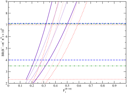
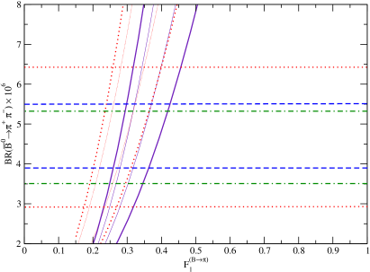
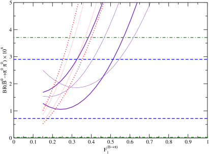
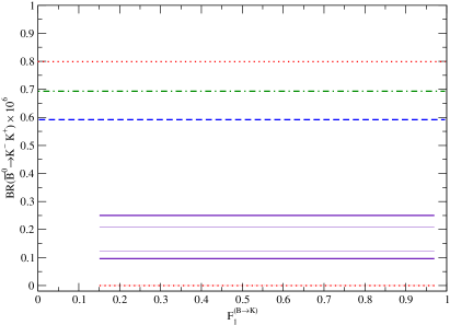
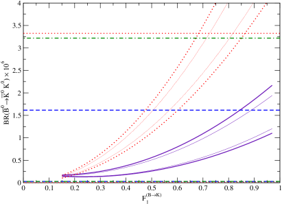
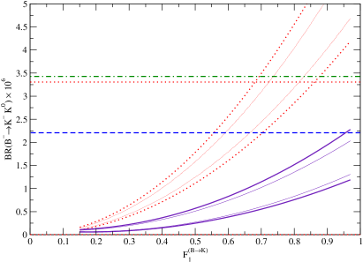
Figure 5: From top left-handed to bottom right-handed, branching ratios $\mathcal{BR}(B^{-}\to\pi^{-}\pi^{0}),\mathcal{BR}(\bar{B}^{0}\to\pi^{+}\pi^{-}),\mathcal{BR}(\bar{B}^{0}\to\pi^{0}\pi^{0}),\mathcal{BR}(\bar{B}^{0}\to K^{-}K^{+}),\mathcal{BR}(\bar{B}^{0}\to\bar{K}^{0}K^{0}),$ $\mathcal{BR}(B^{-}\to K^{-}K^{0})$, as a function of CKM matrix elements and form factors $F^{B\to\pi}$ or $F^{B\to K}$. Solid line(dotted line) for QCDF(NF) factorization and for limiting values of the CKM matrix element parameters shown respectively at 68% (thin line) and 95% (thick line) of confidence level. Notation: horizontal dotted lines: CLEO data; horizontal dashed lines: BABAR data; horizontal dot-dashed lines: BELLE data.

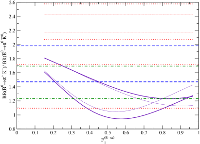
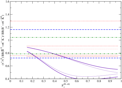
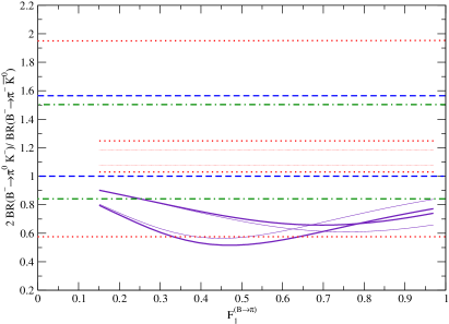
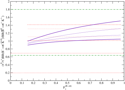
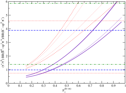
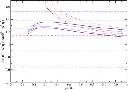
Figure 13: From top left-handed to bottom right-handed, branching ratios for $\mathcal{BR}(\bar{B}^{0}\to\pi^{+}K^{-})/\mathcal{BR}(\bar{B}^{0}\to\pi^{0}\bar{K}^{0}),\mathcal{BR}(\bar{B}^{0}\to\pi^{+}K^{-})/\mathcal{BR}(B^{-}\to\pi^{-}\bar{K}^{0}),2\mathcal{BR}(B^{-}\to\pi^{0}K^{-})/\mathcal{BR}(B^{-}\to\pi^{-}\bar{K}^{0}),\mathcal{BR}(B^{-}\to\pi^{-}\bar{K}^{\ast 0})/\mathcal{BR}(\bar{B}^{0}\to\pi^{+}K^{\ast-}),\mathcal{BR}(\bar{B}^{0}\to\rho^{\pm}\pi^{\mp})/$ $\mathcal{BR}(B^{-}\to\rho^{0}\pi^{-}),\mathcal{BR}(B^{-}\to K^{-}\eta^{\prime})/\mathcal{BR}(\bar{B}^{0}\to\bar{K}^{0}\eta^{\prime}),$ as a function of CKM matrix elements and form factors $F^{B\to\pi}$ or $F^{B\to K}$. Solid line(dotted line) for QCDF(NF) factorization and for limiting values of the CKM matrix element parameters shown respectively at 68% (thin line) and 95% (thick line) of confidence level. Notation: horizontal dotted lines: CLEO data; horizontal dashed lines: BABAR data; horizontal dot-dashed lines: BELLE data.

All the experimental branching ratios for $B$ decays are given in Tables 2, 3, 4 and 5 for $B\to XK$, $B\to X\pi$, $B\to\pi K$ and the ratios of $\mathcal{BR}(B\to XK)$/$\mathcal{BR}(B\to X\pi)$, respectively. All the theoretical branching ratios are plotted from Fig. 5 to Fig. 13 as a function of the form factors, $F^{B\to\pi}$ or $F^{B\to K}$. The variations of the branching ratios with the CKM matrix parameters, $\rho$ and $\eta$, are taken into account in our graphs. Finally, in the case of the naive factorization, we use $N_{c}^{eff}=3$ for the effective parameter. The reason is to clearly show the differences (the hard scattering spectator and annihilations contributions) arising between the two factorization approaches, NF and QCDF.

7.1.1 $\boldsymbol{B\to X\pi}$ with $\boldsymbol{X=\{\rho,\omega,\eta^{(^{\prime})},\pi,K^{*},\phi\}}$

Let us start by analyzing the branching ratios of $B$ decay channels $B\to X\pi$ where $X$ holds for the particles $\rho,\omega,\eta^{(^{\prime})},\pi,K^{*}$ or $\phi$. In Table 6, are listed the different values for the hard-scattering (annihilation) phases, $\varphi_{H}^{M_{i}}(\varphi_{A}^{M_{i}})$, and parameters, $\varrho_{H}^{M_{i}}(\varrho_{A}^{M_{i}})$. The values are given for each of the following particles $(M_{i})$, $\rho,\omega,\eta^{(^{\prime})},\pi,K^{*}$ and $\phi$, and for the minimal (set 2) and maximal (set 1) sets of CKM parameters $\rho$ and $\eta$. All the experimental results from the BELLE, BABAR and CLEO factories for $B\to X\pi$ decays are listed in Tables 3 and 5. The theoretical branching ratios calculated with the NF and QCDF factorizations are shown in Tables 7 and 8. The annihilation and hard scattering spectator contributions are explicitly given in these tables.

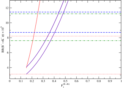
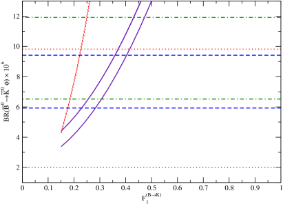
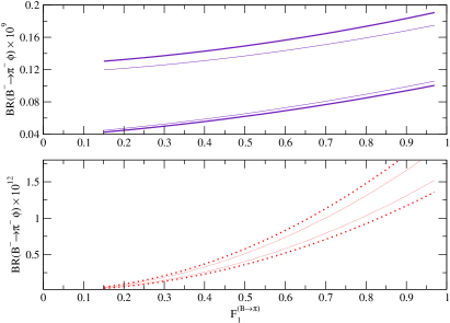
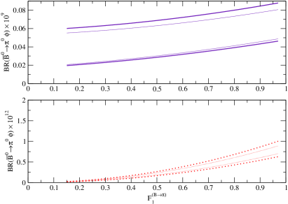
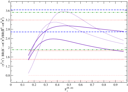
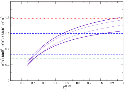
Figure 12: From top left-handed to bottom right-handed, branching ratios $\mathcal{BR}(B^{-}\to K^{-}\phi),\mathcal{BR}(\bar{B}^{0}\to\bar{K}^{0}\phi),\mathcal{BR}(B^{-}\to\pi^{-}\phi),\mathcal{BR}(\bar{B}^{0}\to\pi^{0}\phi),\mathcal{BR}(B^{-}\to\pi^{-}\pi^{0})/\mathcal{BR}(\bar{B}^{0}\to\pi^{0}\pi^{0}),\mathcal{BR}(\bar{B}^{0}\to\pi^{+}\pi^{-})/2\mathcal{BR}(B^{-}\to\pi^{-}\pi^{0})$, as a function of CKM matrix elements and form factors $F^{B\to\pi}$ or $F^{B\to K}$. Solid line(dotted line) for QCDF(NF) factorization and for limiting values of the CKM matrix element parameters shown respectively at 68% (thin line) and 95% (thick line) of confidence level. Notation: horizontal dotted lines: CLEO data; horizontal dashed lines: BABAR data; horizontal dot-dashed lines: BELLE data.

For the decay channel $B\to\pi\pi$, our results are shown in Figs. 5 and 12. It appears that there are no large discrepancies between the NF and QCDF approaches when the form factor, $F^{B\to\pi}$, is within the range 0.24-0.35. Both frameworks yield agreement with the experimental results given by the BELLE, BABAR and CLEO (BBC) measurements as well as with the different experimental constraints for the CKM matrix parameters, $\rho$ and $\eta$ when the form factor, $F^{B\to\pi}$, takes values within 0.24-0.34. We underline that the strong dependence of the branching ratios for $B\to\pi\pi$ on the form factor, $F^{B\to\pi}$, provides an excellent test for the QCDF framework if we assume correct the value obtained for the form factor, $F^{B\to\pi}$. The weak contribution of the annihilation terms does not increase the dependence of these branching ratios on the CKM matrix parameters $\rho$ and $\eta$. The annihilation contribution is even equal to zero in the case of $B^{-}\to\pi^{-}\pi^{0}$. Regarding the ratios of $\mathcal{BR}(B^{-}\to\pi^{-}\pi^{0})/\mathcal{BR}(\bar{B}^{0}\to\pi^{0}\pi^{0})$ and $\mathcal{BR}(\bar{B}^{0}\to\pi^{+}\pi^{-})/\linebreak\mathcal{BR}(B^{-}\to\pi^{-}\pi^{0})$, plotted in Fig. 12, NF and QCDF do not show any agreement. The experimental and NF results only agree for a very limited set of values of the CKM matrix parameters, $\rho$ and $\eta$. A full agreement with the BBC results is found when the QCDF approach is applied. Note as well that the dependence of these ratios on the form factor, $F^{B\to\pi}$, vanishes with the NF approach but remains when QCDF is used because of the inclusion of the annihilation terms.

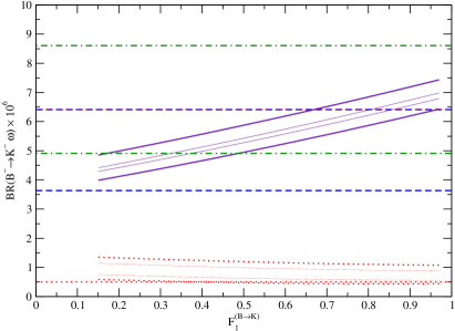
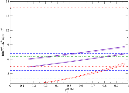
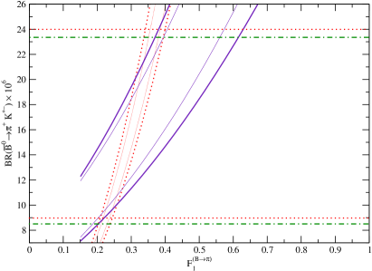
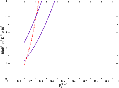
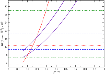
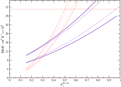
Figure 10: From top left-handed to bottom right-handed, branching ratios $\mathcal{BR}(B^{-}\to K^{-}\omega),\mathcal{BR}(\bar{B}^{0}\to\bar{K}^{0}\omega),\mathcal{BR}(\bar{B}^{0}\to\pi^{+}K^{\ast-}),\mathcal{BR}(\bar{B}^{0}\to\pi^{0}\bar{K}^{\ast 0}),\mathcal{BR}(B^{-}\to\pi^{-}\bar{K}^{\ast 0}),$ $\mathcal{BR}(B^{-}\to\pi^{0}K^{\ast-})$, as a function of CKM matrix elements and form factors $F^{B\to\pi}$ or $F^{B\to K}$. Solid line(dotted line) for QCDF(NF) factorization and for limiting values of the CKM matrix element parameters shown respectively at 68% (thin line) and 95% (thick line) of confidence level. Notation: horizontal dotted lines: CLEO data; horizontal dashed lines: BABAR data; horizontal dot-dashed lines: BELLE data.

For the $B\to\pi K^{*}$ decay channel, our results are shown in Figs. 10 and 13. The agreement between NF and QCDF appears only at values of the form factor, $F^{B\to\pi}\approx 0.2-0.3$, whereas for higher values of $F^{B\to\pi}$, NF predicts larger branching ratios than QCDF. All the BBC experimental results coincide with the theoretical one coming from QCDF when the values of $F^{B\to\pi}$ are about 0.3. The sensitivity of the branching ratios for the $B\to\pi K^{*}$ decays to the CKM matrix parameters, $\rho$ and $\eta$, is much stronger in the case of QCDF than NF, because of the insertion of the annihilation term contribution in the first approach. The strong dependence of the branching ratios on the form factor, $F^{B\to\pi}$, arises either from the only presence of $F^{B\to\pi}$ in the amplitude or from the term $\alpha_{1}F^{B\to\pi}$ (color tree amplitude) when the form factor, $A_{0}^{B\to K^{\ast}}$ is involved. Regarding $\mathcal{BR}(\bar{B}^{0}\to\pi^{0}\bar{K}^{*0})$ and $\mathcal{BR}(B^{-}\to\pi^{0}\bar{K}^{*-})$, we estimate their magnitudes at $3.8\times 10^{-6}$ and $12\times 10^{-6}$, respectively. These last values remain below the branching ratio upper limits only given by the CLEO factory. For the ratio $\mathcal{BR}(B^{-}\to\pi^{-}\bar{K}^{*0})/\mathcal{BR}(\bar{B}^{0}\to\pi^{+}K^{*-})$, an agreement is found between NF and QCDF for all values of $F^{B\to\pi}$ but with the BELLE data only. Our results do not agree with the CLEO ones. The NF approach (in contrast with QCDF) provides a ratio which is independent of the form factor, $F^{B\to\pi}$, because of the annihilation terms.

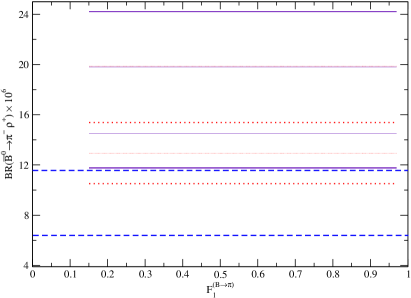
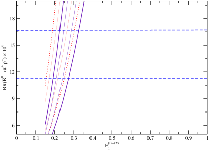
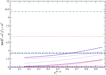
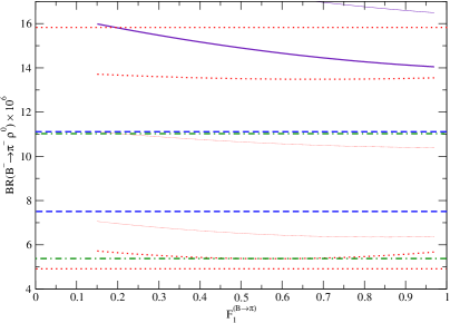
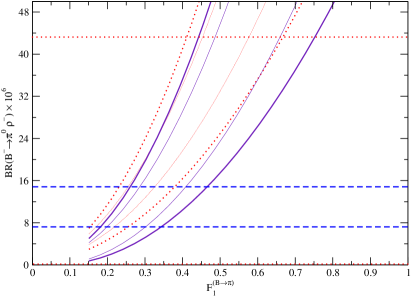
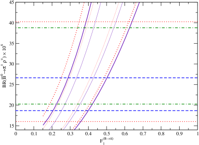
Figure 8: From top left-handed to bottom right-handed, branching ratios $\mathcal{BR}(\bar{B}^{0}\to\pi^{-}\rho^{+}),\mathcal{BR}(\bar{B}^{0}\to\pi^{+}\rho^{-}),\mathcal{BR}(\bar{B}^{0}\to\pi^{0}\rho^{0}),\mathcal{BR}(B^{-}\to\pi^{-}\rho^{0}),\mathcal{BR}(B^{-}\to\pi^{0}\rho^{-}),$ $\mathcal{BR}(\bar{B}^{0}\to\rho^{\pm}\pi^{\mp})$, as a function of CKM matrix elements and form factors $F^{B\to\pi}$ or $F^{B\to K}$. Solid line(dotted line) for QCDF(NF) factorization and for limiting values of the CKM matrix element parameters shown respectively at 68% (thin line) and 95% (thick line) of confidence level. Notation: horizontal dotted lines: CLEO data; horizontal dashed lines: BABAR data; horizontal dot-dashed lines: BELLE data.

Next, we turn to the decay channel $B\to\pi\rho$, for which the results are shown in Figs. 8 and 13. First, let us recall that $B\to\pi\rho$ is governed by the tree topology. Therefore it provides a direct access to the $|V_{ub}|$ and $|V_{ud}|$ CKM matrix elements. The QCDF and NF frameworks do agree with each other for the branching ratios of $B^{-}\to\pi^{0}\rho^{-},\bar{B}^{0}\to\pi^{+}\rho^{-},\bar{B}^{0}\to\pi^{\pm}\rho^{\mp}$ and $\bar{B}^{0}\to\pi^{-}\rho^{+}$, whereas no agreement is observed for $\bar{B}^{0}\to\pi^{0}\rho^{0},B^{-}\to\rho^{0}\pi^{-}$. as well as for the ratio $\mathcal{BR}(\bar{B}^{0}\to\rho^{\pm}\pi^{\mp})/\mathcal{BR}(B^{-}\to\rho^{0}\pi^{-})$. Experimental results provided by BBC coincide with the theoretical results if the form factor, $F^{B\to\pi}$, takes values from 0.2 to 0.4, for $B$ decaying into $\pi^{0}\rho^{-},\pi^{+}\rho^{-},\pi^{\mp}\rho^{\pm}$. For the remaining decays, i.e. for $\pi^{0}\rho^{0},\pi^{-}\rho^{+}$ and $\rho^{0}\pi^{-}$, the agreement between the BBC results and our results are not so clear. Moreover, these branching ratios are weakly (or even not at all) sensitive to the form factor, $F^{B\to\pi}$: this is either because of the form factor, $A_{0}^{B\to\rho}$, in the amplitude or because the main contribution comes from the color power suppressed tree diagram. We note as well a strong dependence of some branching ratios (i.e. $\pi^{-}\rho^{+},\rho^{0}\pi^{-}$) on the CKM matrix parameters, $\rho$ and $\eta$. Such $B$ decay channels are usually required for constraining the CKM matrix because of their high sensitivity to the parameters $\rho$ and $\eta$. Finally, the theoretical ratio $\mathcal{BR}(\bar{B}^{0}\to\rho^{\pm}\pi^{\mp})/\mathcal{BR}(B^{-}\to\rho^{0}\pi^{-})$ agrees with the BBC data for values of the form factor, $F^{B\to\pi}$, larger than 0.2.

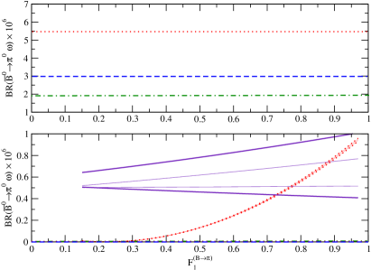
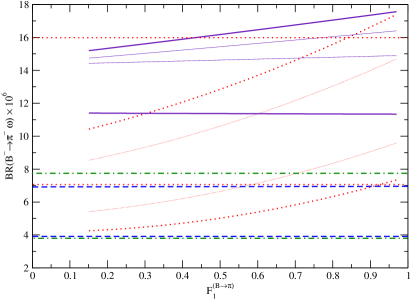
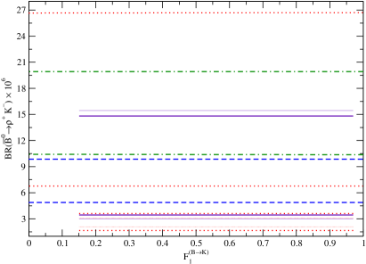
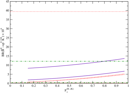
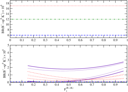
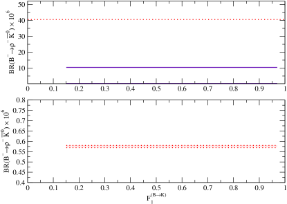
Figure 9: From top left-handed to bottom right-handed, branching ratios $\mathcal{BR}(\bar{B}^{0}\to\pi^{0}\omega),\mathcal{BR}(B^{-}\to\pi^{-}\omega),\mathcal{BR}(\bar{B}^{0}\to\rho^{+}K^{-}),\mathcal{BR}(\bar{B}^{0}\to\rho^{0}\bar{K}^{0}),\mathcal{BR}(B^{-}\to\rho^{0}K^{-}),$ $\mathcal{BR}(B^{-}\to\rho^{-}\bar{K}^{0})$, as a function of CKM matrix elements and form factors $F^{B\to\pi}$ or $F^{B\to K}$. Solid line(dotted line) for QCDF(NF) factorization and for limiting values of the CKM matrix element parameters shown respectively at 68% (thin line) and 95% (thick line) of confidence level. Notation: horizontal dotted lines: CLEO data; horizontal dashed lines: BABAR data; horizontal dot-dashed lines: BELLE data.

In Fig. 9, is plotted the decay channel $B\to\pi\omega$. The NF and QCDF frameworks present similar results only for values of $F^{B\to\pi}$ larger than 0.35 and 0.7 for the decays $\pi^{-}\omega$ and $\pi^{0}\omega$, respectively. Our results for $\pi^{0}\omega$ are below the upper experimental limits given by BBC. For $\pi^{-}\omega$, our results agree with the CLEO data in the case of QCDF and with BELLE and BABAR if NF is used. The similar sensitivity of the branching ratio for $B\to\pi^{-}\omega$ to the CKM parameters, $\rho$ and $\eta$, when NF or QCDF are applied, comes from the small effect of the annihilation contribution. However, this does not hold for the $\pi^{0}\omega$ decay. Our prediction for the branching ratio of $\pi^{0}\omega$ is around $0.6\;10^{-6}$.

Regarding the decay channel $B\to\pi\phi$, our results are shown in Fig. 12. First, let us note that this channel gives one of the smallest branching ratio in $B$ decays because of the penguin dominant contribution. In fact, only the element, $\alpha_{3}$, (from QCD and electroweak QCD penguin diagrams) contributes to the amplitude. Moreover, the NF and QCDF approaches provide very different results for such decay channel since that difference, in terms of magnitude, is of the order $10^{3}$. This difference cannot result from the annihilation term (they do not take part of the amplitude) but from the way of computing the Wilson coefficients. Our theoretical predictions are $1.0\;10^{-9}$ and $0.5\;10^{-9}$ for $B^{-}\to\pi^{-}\phi$ and $\bar{B}^{0}\to\pi^{0}\phi$.

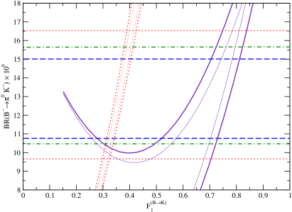
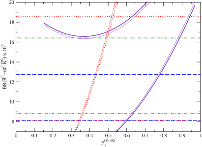
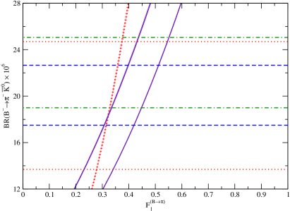
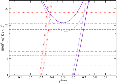
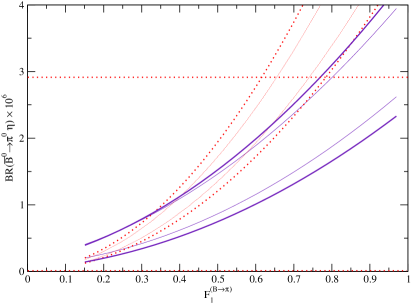
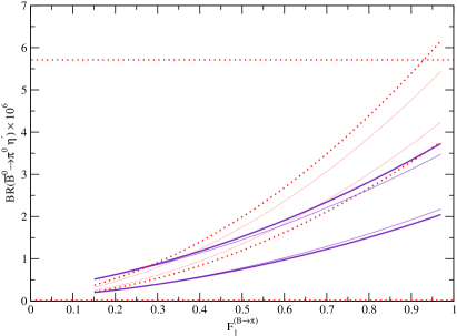
Figure 6: From top left-handed to bottom right-handed, branching ratios $\mathcal{BR}(B^{-}\to\pi^{0}K^{-}),\mathcal{BR}(\bar{B}^{0}\to\pi^{0}\bar{K}^{0}),\mathcal{BR}(B^{-}\to\pi^{-}\bar{K}^{0}),\mathcal{BR}(\bar{B}^{0}\to\pi^{+}K^{-}),\mathcal{BR}(\bar{B}^{0}\to\pi^{0}\eta),$ $\mathcal{BR}(\bar{B}^{0}\to\pi^{0}\eta^{\prime})$, as a function of CKM matrix elements and form factors $F^{B\to\pi}$ or $F^{B\to K}$. Solid line(dotted line) for QCDF(NF) factorization and for limiting values of the CKM matrix element parameters shown respectively at 68% (thin line) and 95% (thick line) of confidence level. Notation: horizontal dotted lines: CLEO data; horizontal dashed lines: BABAR data; horizontal dot-dashed lines: BELLE data.

The last decay channel analyzed in this section is $B\to\pi\eta^{(^{\prime})}$. Our results have been plotted in Figs. 6 and 7. We observe a global agreement between the NF and QCDF factorizations for the four decays, $\pi^{0}\eta^{(\prime)}$ and $\pi^{-}\eta^{(\prime)}$. However, this agreement holds for values of $F^{B\to\pi}$ about 0.2-0.4 if $\pi^{0}\eta^{(\prime)}$ whereas it holds for all possible values of $F^{B\to\pi}$ if $\pi^{-}\eta^{(\prime)}$. In both cases, we have a good agreement between the experimental data given by BBC and our results. For the branching ratios $\bar{B}^{0}\to\pi^{0}\eta$ and $\bar{B}^{0}\to\pi^{0}\eta^{\prime}$, our predictions are $0.45\;10^{-6}$ and $0.5\;10^{-6}$, respectively. In regards to the branching ratio $B^{0}\to\pi^{-}\eta^{\prime}$, we obtained $8.1\;10^{-6}$. Finally, we note that the decay channel $B^{-}\to\pi^{-}\eta^{(\prime)}$ is a good candidate for constraining and checking the CKM parameters, $\rho$ and $\eta$, and the form factor $F^{B\to\pi}$, respectively, because of its strong sensitivity to these parameters.

7.1.2 $\boldsymbol{B\to XK}$ with $\boldsymbol{X=\{\rho,\omega,\eta^{(^{\prime})},K,K^{*},\phi\}}$

Now, let us focus on the branching ratios for $B$ decay channels $B\to XK$ where $X$ stands for $\rho,\omega,\eta^{(^{\prime})},K,K^{*}$ or $\phi$. In Table 6, are listed the different values for the hard-scattering (annihilation) phases, $\varphi_{H}^{M_{i}}(\varphi_{A}^{M_{i}})$ and parameters, $\varrho_{H}^{M_{i}}(\varrho_{A}^{M_{i}})$. The values are given for each of the following particles ($M_{i}$), $\rho,\omega,\eta^{(^{\prime})},K,K^{*},\phi$ and for the minimal (set 2) and maximal (set 1) sets of values of the CKM parameters, $\rho$ and $\eta$. All the experimental results from the BBC factories for the $B\to XK$ decays are listed in Tables 2 and 5. The theoretical branching ratios calculated with the NF and QCDF factorizations are shown for comparison in Tables 7 and 8 where the annihilation and hard scattering spectator contributions are given explicitly.

For the decay channel $B\to KK$, our results are shown in Fig. 5. We found no agreement between the QCDF and NF approaches for all the branching ratios $\bar{K}^{0}K^{0}$, $K^{-}K^{+}$ and $K^{-}K^{0}$. All of our results do agree with the upper experimental limits given by the BBC results. Our predictions for the branching ratios, $K^{-}K^{0},K^{-}K^{+}$ and $\bar{K}^{0}K^{0}$ are respectively $0.31\;10^{-6},0.2\;10^{-6}$ and $0.27\;10^{-6}$. It appears that these branching ratios calculated with QCDF are smaller than those with NF because of the sizable contribution of the annihilation terms. Moreover, in the case of $B$ decaying into $K^{-}K^{+}$, the annihilation contribution is the only one which participates in the amplitude. As a result, NF gives a branching ratio equal to zero in the latter case. The same reason explains the independence of this branching ratio on the form factor, $F^{B\to K}$. The dependence of these branching ratios on the CKM parameters, $\rho$ and $\eta$, as well as on the form factor, $F^{B\to K}$, is quite similar in both approaches, i.e. NF and QCDF.

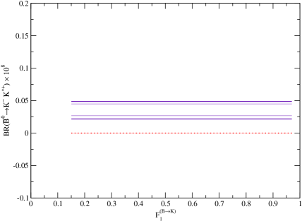
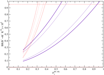
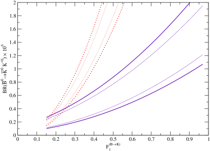
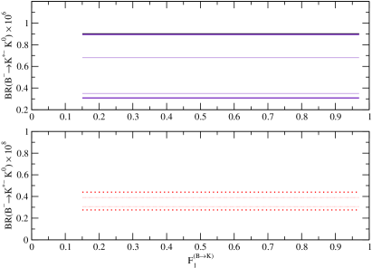
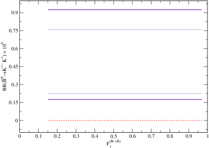
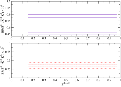
Figure 11: From top left-handed to bottom right-handed, branching ratios $\mathcal{BR}(\bar{B}^{0}\to K^{-}K^{\ast+}),\mathcal{BR}(B^{-}\to K^{-}K^{\ast 0}),\mathcal{BR}(\bar{B}^{0}\to\bar{K}^{0}K^{\ast 0}),\mathcal{BR}(B^{-}\to K^{\ast-}K^{0}),\mathcal{BR}(\bar{B}^{0}\to K^{\ast-}K^{+}),\mathcal{BR}(\bar{B}^{0}\to\bar{K}^{\ast 0}K^{0})$, as a function of CKM matrix elements and form factors $F^{B\to\pi}$ or $F^{B\to K}$. Solid line(dotted line) for QCDF(NF) factorization and for limiting values of the CKM matrix element parameters shown respectively at 68% (thin line) and 95% (thick line) of confidence level. Notation: horizontal dotted lines: CLEO data; horizontal dashed lines: BABAR data; horizontal dot-dashed lines: BELLE data.

Our results for the decay channel $B\to KK^{\ast}$ are shown in Fig. 11. Unfortunately, there are no available experimental results for these decays. Only one upper limit is given by CLEO for the decay $K^{-}K^{\ast 0}$. Of the six ways for a $B$ to decay into $KK^{\ast}$, only two branching ratios, $K^{-}K^{\ast 0}$ and $\bar{K}^{0}K^{\ast 0}$, allow one for an agreement between NF and QCDF. However, this agreement holds only at low values of the form factor, $F^{B\to K}$, i.e. about 0.2-0.25. For all the other cases, the NF and QCDF factorization give different branching ratio results. We recall that $B\to KK^{\ast}$ is only governed by the penguin topology. In the case of the $K^{-}K^{\ast+}$ and $K^{\ast-}K^{+}$ decays, the magnitude of their branching ratios comes from the annihilation contribution alone. That explains the independence of these branching ratios on the form factor, $F^{B\to K}$, as well as the fact that NF gives magnitudes equal to zero. Regarding the decays $K^{\ast-}K^{0}$ and $K^{-}K^{\ast 0}$, there is a factor $10^{2}$ and $10^{1}$, respectively, between the results obtained with NF and QCDF. The non sensitivity of these branching ratios to the form factor, $F^{B\to K}$, arises from the only contribution of the form factor $F^{B\to K^{\ast}}$ in the amplitude. Because of the annihilation terms, a stronger dependence of the branching ratios on the CKM parameters, $\rho$ and $\eta$, is observed when QCDF is applied. Finally, we predict the branching ratios for $\bar{K}^{0}K^{\ast 0},\bar{K}^{\ast 0}K^{0},K^{-}K^{\ast+},K^{\ast-}K^{+},K^{-}K^{\ast 0}$ and $K^{\ast-}K^{0}$ to be of the order $0.4\;10^{-6},0.75\;10^{-6},3.0\;10^{-6},0.6\;10^{-6},0.4\;10^{-6}$ and $0.68\;10^{-6}$, respectively.

We have plotted in Fig. 9 the decay channel $B\to K\rho$. Experimental results provided by BBC are well reproduced and all of our results are below the upper limits given for the branching ratio data. No strong agreement between NF and QCDF can be confirmed. A weak (or even no) dependence of these branching ratios on the form factor, $F^{B\to K}$, is observed. This is either due to the interference of the form factor, $F^{B\to K}$, with the form factor $A_{0}^{B\to\rho}$ (enhanced by a color-allowed tree diagram, $\alpha_{1}$) or the absence of the $B\to K$ transition in the amplitude. We also note a stronger sensitivity of the branching ratios to the CKM parameters, $\rho$ and $\eta$, in the case where the annihilation terms are taken into account. We conclude by giving our results regarding this channel: $5.8\;10^{-6},5.0\;10^{-6}$ and $1.7\;10^{-6}$ are respectively our predicted branching ratios for $\rho^{0}\bar{K}^{0},\rho^{-}\bar{K}^{0}$ and $\rho^{0}K^{-}$.

Next, we consider the decay channel, $B\to K\omega$, for which the results are shown in Fig. 10. As already the case for $B\to K\rho$, no agreement between the NF and QCDF frameworks is observed. However, the accurate experimental results given by the BBC factories coincide with the branching ratios obtained with QCDF when the form factor, $F^{B\to K}$, is in the range of values 0.2-0.45. The differences between the two frameworks come from the contribution of the annihilation terms which strongly enhance the magnitude of these branching ratios. The sensitivity to the CKM parameters, $\rho$ and $\eta$, arises from the annihilation contribution as well.

For the decay channel, $B\to K\phi$, our results are shown in Fig. 12. The QCDF factorization agrees with the overlap of experimental data for values of the form factor, $F^{B\to K}$, equal to 0.2-0.5. We observe a very similar behaviour between the two decays, $K^{-}\phi$ and $\bar{K}^{0}\phi$. The small difference only comes from the annihilation contribution. We underline as well a better sensitivity to the CKM parameters, $\rho$ and $\eta$, in the case where QCDF is applied. The latter behaviour is still due to the annihilation term. Finally, we note a strong dependence of the branching ratios on the form factor, $F^{B\to K}$. It may be a good channel for checking the form factor, $F^{B\to K}$, if we assume correct the factorization procedure or vice-versa. However, the magnitude of this decay channel remains very small because it is dominated by penguin diagram.

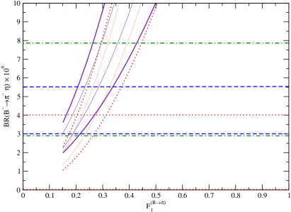
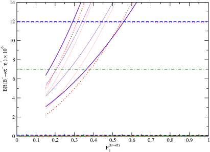
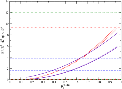
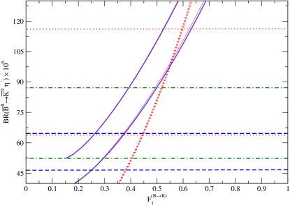
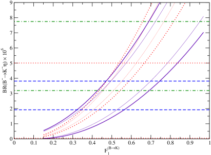
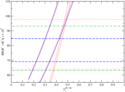
Figure 7: From top left-handed to bottom right-handed, branching ratios $\mathcal{BR}(B^{-}\to\pi^{-}\eta),\mathcal{BR}(B^{-}\to\pi^{-}\eta^{\prime}),\mathcal{BR}(\bar{B}^{0}\to\bar{K}^{0}\eta),\mathcal{BR}(\bar{B}^{0}\to\bar{K}^{0}\eta^{\prime}),\mathcal{BR}(B^{-}\to K^{-}\eta),\mathcal{BR}(B^{-}\to K^{-}\eta^{\prime})$, as a function of CKM matrix elements and form factors $F^{B\to\pi}$ or $F^{B\to K}$. Solid line(dotted line) for QCDF(NF) factorization and for limiting values of the CKM matrix element parameters shown respectively at 68% (thin line) and 95% (thick line) of confidence level. Notation: horizontal dotted lines: CLEO data; horizontal dashed lines: BABAR data; horizontal dot-dashed lines: BELLE data.

The last decay channel which we investigate is $B\to K\eta^{(^{\prime})}$, for which our results are shown in Figs. 7 and 13 . The decays $K^{-}\eta$ and $\bar{K}^{0}\eta$ show good agreement between the NF and QCDF approaches for almost all values of the form factor, $F^{B\to K}$, whereas the decays $K^{-}\eta^{\prime}$ and $\bar{K}^{0}\eta^{\prime}$ do not. The experimental branching ratios and theoretical results agree with each other when the form factor, $F^{B\to K}$, is about 0.35 for $K\eta^{\prime}$ decays and about 0.55 for $K\eta$ decays. We observe a stronger sensitivity of the branching ratios to the CKM parameters when the QCDF factorization is used. It has to be noticed that the decay channel $K\eta^{\prime}$ is an excellent candidate for the determination of both of the CKM parameters, $\rho$ and $\eta$, and the form factor, $F^{B\to K}$. This statement holds if the procedure of factorization and the evaluation of the annihilation contribution are assumed to be correct. Moreover, the last decay channel is one order of magnitude bigger than those usually observed in $B$ decays. That makes its determination easier and accurate results are expected, thanks to the BBC factories. We also predict a branching ratio for the decay $\bar{K}^{0}\eta$ to be of the order $0.9\;10^{-6}$. Finally, the ratio $\mathcal{BR}(B^{-}\to K^{-}\eta^{\prime})/\mathcal{BR}(\bar{B}^{0}\to\bar{K}^{0}\eta^{\prime})$ shows an agreement between NF and QCDF at large values of the form factor, $F^{B\to K}$, only. However, QCDF agrees with the BELLE and BABAR data at values of $F^{B\to K}$ about 0.35. No agreement is found with CLEO.

7.1.3 $\boldsymbol{B\to\pi K}$

We conclude our analysis of branching ratios for $B$ decay channels including a pion (or a kaon) and another meson in the final state by turning to those where both the kaon and pion are in the final state. The experimental results corresponding to the $B\to\pi K$ decays are given in Tables 4 and 5. The theoretical branching ratios including the annihilation and hard scattering spectator contributions are given for comparison in Table 8.

In Figs. 6 and 13 we show the results for the decay channel $\pi K$. We first observe a different behaviour between the NF and QCDF approaches. This is due to the annihilation contribution which strongly enhances these branching ratios. As a result, NF and QCDF only coincide to each other for a small set of values of the form factors, $F^{B\to K}$, and $F^{B\to\pi}$, which are of the order 0.3-0.4. We note as well an excellent agreement between our results and the branching ratio data provided by the BBC factories. The strong dependence of the branching ratios for the decays $\pi K$ on the CKM parameters, $\rho$ and $\eta$, when QCDF is applied, gives one the opportunity to efficiently constrain these latter parameters. At the same time, it allows us to accurately model the annihilation contribution, since it arises in the amplitude times a CKM matrix element $V_{pb}V_{pD}^{\ast}$ (in the case of $b\to d$ transition). We finally underline that the sensitivity of this decay channel to the forms factors, $F^{B\to K}$, and $F^{B\to\pi}$, contributes effectively to the tests of the procedure of factorization of $B$ decaying into two light mesons.

Regarding the ratios $\mathcal{BR}(\bar{B}^{0}\to\pi^{+}K^{-})/\mathcal{BR}(\bar{B}^{0}\to\pi^{0}\bar{K}^{0}),\mathcal{BR}(B^{-}\to\pi^{0}K^{-})/\mathcal{BR}(B^{-}\linebreak\to\pi^{-}\bar{K}^{0})$ and $\mathcal{BR}(\bar{B}^{0}\to\pi^{+}K^{-})/\mathcal{BR}(B^{-}\to\pi^{-}\bar{K}^{0})$, no agreement between NF and QCDF is found. This is not true for the latter ratio if the values of the form factor, $F^{B\to\pi}$, are about 0.15-0.45. Our predictions for these ratios and those given by BBC do reasonably agree. Finally, the ratios calculated within the NF framework do not depend on form factor because of the omission of the annihilation terms, whereas they do when QCDF is used.

Before going further in our analysis, let us draw the main conclusions of this analysis of the branching ratios for $B$ decay channels $B\to\pi X$ and $B\to KX$ where $X=\rho,\omega,\eta^{(^{\prime})},\pi,K,K^{*}$ and $\phi$. We have calculated the branching ratios for $B$ decays into two mesons in the final state where we have made comparison with the NF and QCDF frameworks. The results show that the form factors, $F^{B\to\pi}$ and $F^{B\to K}$, are equal to $0.31\pm 0.12$ and $0.37\pm 0.13$, respectively. At the same time, we have determined the four unknown parameters used in QCDF by performing a fit to all of the branching ratio data provided by the BBC facilities. We note that we did not take into account any $CP$ violating asymmetry experimental values, $a_{CP}^{exp}$, in our fit. These phases, $\varphi_{H,A}^{M_{i}}$, and parameters, $\varrho_{H,A}^{M_{i}}$ are assumed, in our analysis, to be non universal regarding the mesons. It appears that their determination is very sensitive to the values of the CKM parameters, $\rho$ and $\eta$, and unfortunately, at the present time, it is not possible to draw any firm conclusions concerning this point. Let us note that the NF factorization gives, in first approximation, the right order of magnitude of branching ratios in most of the cases. We have used $N_{c}^{eff}=3$ for the effective parameter. This emphasizes the differences between NF and QCDF since, in that case, the differences mainly come from the hard scattering spectator as well as the annihilation terms. In most of the investigated cases, we observed a quite good agreement between NF and QCDF if we restrict the transition form factors, $F^{B\to\pi}$ or $F^{B\to K}$, to the range of values 0.2-0.4. This common behaviour was expected because the non factorizable terms are usually power suppressed corrections (see Eq. (19)). If we use $N_{c}^{eff}=2$ for the effective parameter in NF, our results remain coherent with the previous observation. However, the theoretical branching ratio results obtained by applying the QCDF framework do provide better agreement with the BBC data. This is also due to the annihilation term effects included only in the QCDF approach. It has to be emphasized as well that the latter contribution takes importance if we analyze the dependence of branching ratios on the CKM parameters $\rho$ and $\eta$. Finally, over all the analyzed branching ratios, some of them are more suitable for the analysis of the CKM matrix elements and others for checking the factorization procedure if we assume correct the transition form factors. Let us mention, $\bar{B}^{0}\to\pi^{\pm}\rho^{\mp},B^{-}\to\pi^{0}\rho^{-}$, and $B^{-}\to\pi^{-}\pi^{0},\bar{B}^{0}\to\pi^{+}\pi^{-},\bar{K}^{0}\to\bar{K}^{0}\eta^{\prime}$, respectively. Regarding the effect of the annihilation contribution, the following $B$ decay channels are the most interesting since the amplitude of their branching ratios is only proportional to the annihilation term: $\bar{B}^{0}\to K^{-}K^{+},\bar{B}^{0}\to K^{-}K^{\ast+}$ and $\bar{B}^{0}\to K^{\ast-}K^{+}$.

7.2 $\boldsymbol{CP}$ violating asymmetry

Now, let us focus on the violation of $CP$ symmetry. We concentrate our analysis on $B$ decays such as $B\to\rho^{0}(\omega)M_{2}\to\pi^{+}\pi^{-}M_{2}$, where $M_{2}$ is either a pion or a kaon. It has been shown in previous studies that the CP-violating asymmetry parameter, $a_{CP}$, may be large when the invariant mass $\pi^{+}\pi^{-}$ is in the vicinity of the $\omega$ resonance. This enhancement is known as $\rho-\omega$ mixing effect and we refer interested readers to Refs. [102, 103, 104] for more details. In this last section, we are using all the parameters collected thanks to the analysis of branching ratios of $B$ decays.

In the application of the QCD factorization, we define, for practical reason, three amplitudes, $t^{u},p^{u}$ and $p^{c}$. We set the amplitudes as follows:

$$A_{Bf} =|A_{1}|e^{i\delta_{1}+i\phi_{1}}+|A_{2}|e^{i\delta_{2}+i\phi_{2}}+|A_{3}|e^{i\delta_{3}+i\phi_{3}}\ ,$$

$$\bar{A}_{Bf} =|\bar{A}_{1}|e^{i\delta_{1}-i\phi_{1}}+|\bar{A}_{2}|e^{i\delta_{2}-i\phi_{2}}+|\bar{A}_{3}|e^{i\delta_{3}-i\phi_{3}}\ ,$$ (82)

where the first term refers to the “tree” contribution, $A_{1}\equiv t^{u}$, instead of the remaining terms define the “penguin” contributions with $A_{2}\equiv p^{u}$, and $A_{3}\equiv p^{c}$. In that case, the $CP$ violating asymmetry, $a_{CP}$, takes the following form:

$$a_{CP}\equiv\frac{|A|^{2}-|\bar{A}|^{2}}{|A|^{2}+|\bar{A}|^{2}}=\\ \frac{-2(r_{1}\sin\phi_{12}\sin\delta_{12}+r_{2}\sin\phi_{13}\sin\delta_{13}+r_{1}r_{2}\sin\phi_{23}\sin\delta_{23})}{1+r_{1}^{2}+r_{2}^{2}+2(r_{1}\cos\phi_{12}\cos\delta_{12}+r_{2}\cos\phi_{13}\cos\delta_{13}+r_{1}r_{2}\cos\phi_{23}\cos\delta_{23})}\ ,$$ (83)

where the convention for the used parameters is:

$$r_{1}=\left|\frac{A_{2}}{A_{1}}\right|\ ,\;\;\;\;r_{2}=\left|\frac{A_{3}}{A_{1}}\right|\ ,\;\;{\rm and}\;\;\phi_{ij}=\phi_{i}-\phi_{j}\ ,\;\;\;\;\delta_{ij}=\delta_{i}-\delta_{j}\ .$$ (84)

The parameters, $r_{i}$, and the phases, $\delta_{ij}$, are given by applying Eq. (38) whereas $\delta_{23}$ is obtained from the ratio $\lambda_{u}p^{u}/\lambda_{c}p^{c}$ where $\lambda_{p}=V_{pb}V^{*}_{pD}$ with $D=d,s$. Finally, the phases $\phi_{13}=\phi_{23}={\rm arg}[(V_{cb}V_{cd}^{\star})/(V_{ub}V_{ud}^{\star})]$ for $b\to d$ transition, $\phi_{13}=\phi_{23}={\rm arg}[(V_{cb}V_{cs}^{\star})/(V_{ub}V_{us}^{\star})]$ for $b\to s$ transition and $\phi_{12}=0$ in both transitions. $\sin\phi_{13}\;(\cos\phi_{13})$ takes the following form in case of $b\to d$ transition,

$$\sin\phi_{13}=\sin\phi_{23} =\frac{-(\lambda\eta-\frac{1}{2}A^{2}\lambda^{5})}{\sqrt{\left(\eta\lambda-\frac{A^{2}\lambda^{5}}{2}\right)^{2}+\left(\lambda\rho+\frac{1}{2}A^{2}\lambda^{5}(2\eta^{2}+\rho(-1+2\rho))\right)^{2}}}\ ,$$

$$\cos\phi_{13}=\cos\phi_{23} =\frac{\frac{1}{2}A^{2}\lambda^{5}(\rho-2\rho^{2}-2\eta^{2})-\lambda\rho}{\sqrt{\left(\eta\lambda-\frac{A^{2}\lambda^{5}}{2}\right)^{2}+\left(\lambda\rho+\frac{1}{2}A^{2}\lambda^{5}(2\eta^{2}+\rho(-1+2\rho))\right)^{2}}}\ ,$$ (85)

and in case of $b\to s$ transition, $\sin\phi_{13}\;(\cos\phi_{13})$ is given by:

$$\sin\phi_{13}=\sin\phi_{23} =\frac{\eta}{\sqrt{\rho^{2}+\eta^{2}}}\ ,$$

$$\cos\phi_{13}=\cos\phi_{23} =\frac{\rho}{\sqrt{\rho^{2}+\eta^{2}}}\ .$$ (86)

7.2.1 $\boldsymbol{B\rightarrow\rho^{0}(\omega)\pi\to\pi^{+}\pi^{-}\pi}$

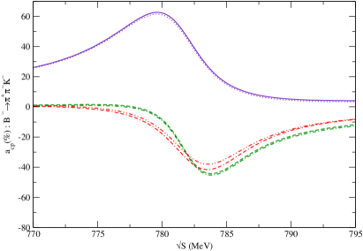
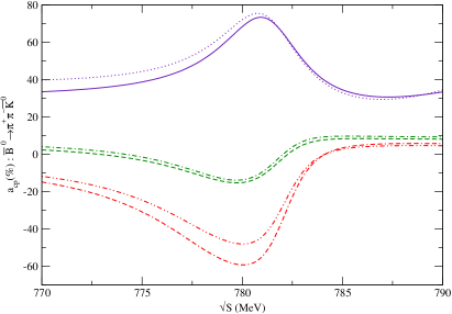
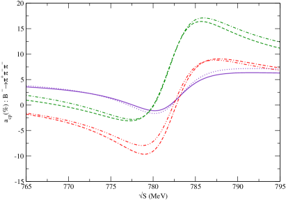
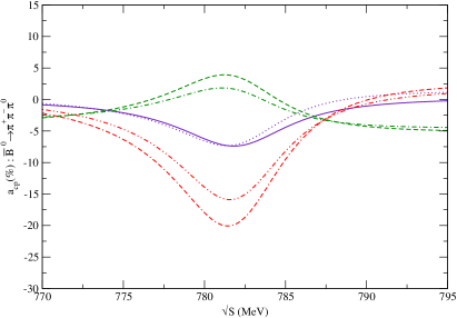
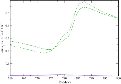
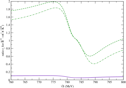
Figure 14: First row, $CP$ violating asymmetry, $a_{CP}$, for $B^{-}\to\pi^{+}\pi^{-}K^{-},\bar{B}^{0}\to\pi^{+}\pi^{-}\bar{K}^{0}$ for max CKM matrix elements. Solid line (dotted line) for QCDF, dot-dot-dashed line (dot-dash-dashed line) for NF, dot-dashed line (dashed line) for QCDF with default values and for $F^{B\to K}=0.35(0.42)$. Second row, $CP$ violating asymmetry, $a_{CP}$, for $B^{-}\to\pi^{+}\pi^{-}\pi^{-},\bar{B}^{0}\to\pi^{+}\pi^{-}\pi^{0}$, for max CKM matrix elements. Same notation for lines as in first row with $F^{B\to\pi}=0.27(0.35)$. Last row, the ratio of penguin to tree amplitudes, $r_{i}$, for $B\to\pi\pi K$, for max CKM matrix elements. Solid line (dotted line) for $r_{1}=p^{u}/t^{u}$, dashed line (dot-dashed line) for $r_{2}=p^{c}/t^{u}$ and for $F^{B\to K}=0.35(0.42)$. All the figures are given as a function of $\sqrt{S}$.

We have investigated the $CP$ violating asymmetry, $a_{CP}$, for the $B$ decays such as $B\rightarrow\rho^{0}(\omega)\pi\to\pi^{+}\pi^{-}\pi$. In Fig. 14, we show the $CP$ violating asymmetry for $B^{-}\to\rho^{0}(\omega)\pi^{-}\to\pi^{+}\pi^{-}\pi^{-}$ and $\bar{B}^{0}\to\rho^{0}(\omega)\pi^{0}\to\pi^{+}\pi^{-}\pi^{0}$ respectively, as a function of the energy, $\sqrt{S}$, of the two pions coming from $\rho^{0}$ decay, the form factor, $F_{1}^{B\to\pi}$, and the CKM matrix element parameters $\rho$ and $\eta$. For comparison, on the same plot we show the $CP$ violating asymmetries, $a_{CP}$, when NF is applied as well as QCDF where default values for the phases, $\varphi_{H,A}^{M_{i}}$, and parameters, $\varrho_{H,A}^{M_{i}}$ are used. In the latter case, we take $\varphi_{H,A}^{M_{i}}=0$ and $\varrho_{H,A}^{M_{i}}=1$ for all the particles.

Focusing first on Fig. 14, where the asymmetry for $B^{-}\to\rho^{0}(\omega)\pi^{-}\to\pi^{+}\pi^{-}\pi^{-}$ is plotted, we observe that the $CP$ violating asymmetry parameter, $a_{CP}$, can be large outside the region where the invariant mass of the $\pi^{+}\pi^{-}$ pair is in the vicinity of the $\omega$ resonance. This is the first consequence of QCD factorization, since within this framework, the strong phase can be generated not only by the $\rho-\omega$ mechanism but also by the Wilson coefficients. We recall that the Wilson coefficients include all of the final state interactions at order $\alpha_{s}$. This shows as well that the non factorizable contribution effects are important and can modify the strong interaction phase. Because of the strong phase that is either at the order of $\alpha_{s}$ or power suppressed by $\Lambda_{QCD}/m_{b}$, the $CP$ violating asymmetry, $a_{CP}$, may be small but a large asymmetry cannot be excluded.

At the $\omega$ resonance, the asymmetry parameter, $a_{CP}$, for $B^{-}\to\pi^{+}\pi^{-}\pi^{-}$, is around $0\%$ in our case. In comparison, the asymmetry parameter, $a_{CP}$, (still at the $\omega$ resonance) obtained by applying the naive factorization gives $-10\%$ whereas it gives $-2\%$ in case of QCDF with default values for $\varphi_{H,A}^{M_{i}}$ and $\varrho_{H,A}^{M_{i}}$. The results are quite different between these approaches because of the strong phase mentioned previously. On the same figure, the asymmetry violating parameter, $a_{CP}$, is shown for the decay $\bar{B}^{0}\to\pi^{+}\pi^{-}\pi^{0}$ as a function of $\sqrt{S}$, the form factor, $F^{B\to\pi}$, and for one set of CKM parameters, $\rho$ and $\eta$. In the vicinity of the $\omega$ resonance, the QCDF approach gives an asymmetry of the order $-8\%$. We obtain $-20\%$ and $+5\%$ in the case of NF and QCDF with the default values for $\varphi_{H,A}^{M_{i}}$ and $\varrho_{H,A}^{M_{i}}$.

It appears as well that the asymmetry depends strongly on the CKM matrix parameters $\rho$ and $\eta$, as expected. When QCDF is applied, the asymmetry for the decay $B^{-}\to\pi^{+}\pi^{-}\pi^{-}$, varies from $12\%$ to $+5\%$ outside the region of the $\omega$ resonance whereas for the decay $\bar{B}^{0}\to\pi^{+}\pi^{-}\pi^{0}$, the asymmetry varies from $10\%$ down to $-20\%$, depending on the CKM matrix element parameters, $\rho$ and $\eta$. In the vicinity of the $\omega$ resonance, the asymmetry, $a_{CP}$, takes values from $-2\%$ to $5\%$ for $B^{-}\to\pi^{+}\pi^{-}\pi^{-}$ and from $5\%$ to $-30\%$ for $\bar{B}^{0}\to\pi^{+}\pi^{-}\pi^{0}$ when $\rho$ and $\eta$ vary. In both decays, we note as well a dependence of the asymmetry on the form factor, $F^{B\to\pi}$. This dependence reaches usually its maximum when the asymmetry is given at the $\omega$ resonance. However, this dependence remains under control because of the constraints obtained for their values by the analysis of $B$ branching ratios.

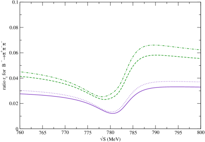
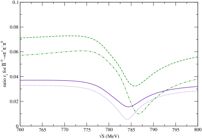
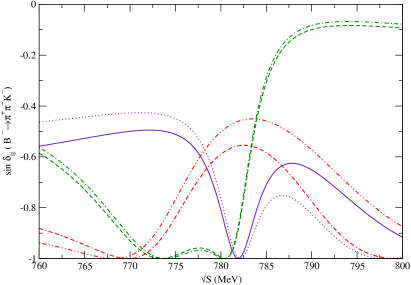
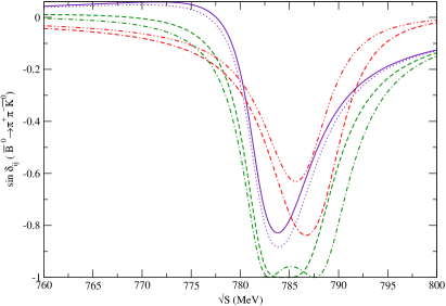
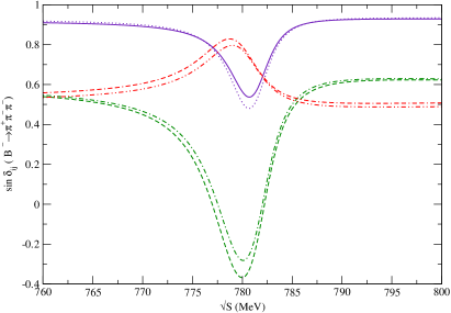
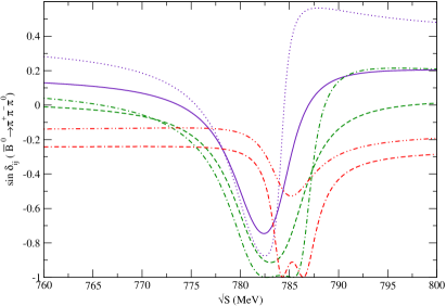
Figure 15: First row, the ratio of penguin to tree amplitudes, $r_{i}$, for $B\to\pi\pi\pi$, for max CKM matrix elements. Solid line (dotted line) for $r_{1}=p^{u}/t^{u}$, dashed line (dot-dashed line) for $r_{2}=p^{c}/t^{u}$ and for $F^{B\to\pi}=0.27(0.35)$. Second and last row, solid line (dotted line) for $\sin\delta_{12}$, dot-dot-dashed line (dot-dash-dashed line) for $\sin\delta_{23}$, and dashed line (dot-dashed line) for $\sin\delta_{13}$ for $F^{B\to K}=0.35(0.42)$ or $F^{B\to\pi}=0.27(0.35)$ according to the given decay. All the figures are given as a function of $\sqrt{S}$.

In Fig. 15, the ratio, $r_{i}$, of penguin to tree amplitude for $B\to\pi^{+}\pi^{-}\pi$ is given as a function of $\sqrt{S}$, the form factor $F^{B\to\pi}$ and for one set of CKM parameter, $\rho$ and $\eta$. For both decays, i.e. $B^{-}\to\pi^{+}\pi^{-}\pi^{-}$ and $\bar{B}^{0}\to\pi^{+}\pi^{-}\pi^{0}$ we observe similar results for $r_{1}=p^{u}/t^{u}$ and $r_{2}=p^{c}/t^{u}$. As is expected for dominant tree decays, the contribution coming from the tree diagram, $t^{u}$, is bigger than that one coming from the penguins, $p^{u}$ or $p^{c}$. Finally, as mentioned, one of the main reasons for the interest in $\rho-\omega$ mixing is to provide an opportunity to remove the phase uncertainty mod$(\pi)$ in the determination of the CKM angle $\alpha$ in the case of $b\to u$ transition. Knowing the sign of the $CP$ violating asymmetry at the $\omega$ resonance gives us the angle $\alpha$ without any ambiguity. In Fig. 15, we present the evolution of $\sin\delta_{12},\sin\delta_{13}$ and $\sin\delta_{23}$ as a function of $\sqrt{S}$, the form factor $F^{B\to\pi}$ and for one set of CKM parameters $\rho$ and $\eta$. In both decays, $\sin\delta_{ij}$ goes to a maximum or a minimum when $\sqrt{S}$ is in the vicinity of the $\omega$ resonance.

7.2.2 $\boldsymbol{B\rightarrow\rho^{0}(\omega)K\to\pi^{+}\pi^{-}K}$

After the analysis of the $CP$ asymmetry in $B^{\pm,0}\to\rho^{0}(\omega)\pi^{\pm,0}\rightarrow\pi^{+}\pi^{-}\pi^{\pm,0}$, we conclude our work by focusing on the asymmetry in $B^{\pm,0}\rightarrow\pi^{+}\pi^{-}K^{\pm,0}$. Plotted in Fig. 14 is the direct $CP$ violating asymmetry, $a_{CP}$, for $B^{-}\to\rho^{0}(\omega)K^{-}\to\pi^{+}\pi^{-}K^{-}$ and for $\bar{B}^{0}\to\rho^{0}(\omega)\bar{K}^{0}\to\pi^{+}\pi^{-}\bar{K}^{0}$, as a function of $\sqrt{S}$, the form factor, $F^{B\to K}$, and for one set of CKM parameters $\rho$ and $\eta$.

For the decay $B^{-}\to\pi^{+}\pi^{-}K^{-}$, the asymmetry, $a_{CP}$, in the vicinity of the $\omega$ resonance, is about $+60\%$ with QCDF, $-40\%$ with NF and $-45\%$ with QCDF and default values for $\varphi_{H,A}^{M_{i}}$ and $\varrho_{H,A}^{M_{i}}$. For the decay $\bar{B}^{0}\to\pi^{+}\pi^{-}\bar{K}^{0}$, when $\sqrt{S}$ is near the $\omega$ resonance, the asymmetry, $a_{CP}$ is about $+70\%$ with QCDF, $-60\%$ with NF and $-15\%$ with QCDF and usual default values for $\varphi_{H,A}^{M_{i}}$ and $\varrho_{H,A}^{M_{i}}$. There is no agreement, for the value of the asymmetry between the naive and QCD factorization at the $\omega$ resonance except that, in both cases, the $CP$ violating asymmetry, $a_{CP}$ reaches its maximum in the vicinity of $\omega$. Similar conclusions can be drawn to that of previous case regarding the sensitivity of the asymmetry parameter, $a_{CP}$, on the form factor, $F^{B\to K}$, as well as the CKM matrix element parameters, $\rho$ and $\eta$. In Fig. 14, the ratio, $r_{i}$, of penguin to tree amplitudes, for $\bar{B}^{0}\to\pi\pi\bar{K}^{0}$ and $B^{-}\to\pi\pi K^{-}$ is plotted. We observe that the ratio $r_{1}=p^{u}/t^{u}$ is very small. This underlines the contribution of the tree diagram, $t^{u}$, in comparison with the penguin one, $p^{u}$. We observe as well that the ratio $r_{2}=p^{c}/t^{u}$ is much bigger than $r_{1}=p^{u}/t^{u}$. This is due to an additional contribution of the $c$ quark when the amplitude for $\bar{B}^{0}\to\omega\bar{K}^{0}$ and $B^{-}\to\omega K^{-}$ are calculated (see Eqs. 138 and 139 in Appendix B). As usual, we note that $\rho-\omega$ mixing strongly enhances the ratio, $r_{i}$, at the $\omega$ resonance. As we did for $B$ decaying into $\pi\pi\pi$, we can remove the ambiguity for the determination of the angle $\gamma$ that arises from the conventional determination of $\sin 2\gamma$ in indirect $CP$ violation. In Fig. 15, $\sin\delta_{ij}$, as a function of $\sqrt{S}$, the form factor, $F^{B\to K}$, and for one set of CKM parameters, $\rho$ and $\eta$, for $B\to\pi\pi K$ is shown. For both decays, $\sin\delta_{ij}$, is large in the vicinity of the $\omega$ resonance i.e. around $775-785$ MeV. As for $B\to\pi\pi\pi$, we note that the strong phase, $\delta_{ij}$, can remain large outside the region where the mass of the $\pi^{+}\pi^{-}$ pair is in the vicinity of the $\omega$ resonance. This underlines the dynamical mechanism of creating a strong phase not only at the $\omega$ resonance but for all values of $\sqrt{S}$.

From this analysis, it is clear that to take into account $\rho-\omega$ mixing in $B$ decays such as $B\to\rho(\omega)M_{i}$ allows us to “amplify” the hadronic interaction near the $\omega$ resonance and it provides an excellent test of the Standard Model through direct $CP$ violation.

8 Summary and discussion

The calculation of the hadronic matrix elements that appear in the $B$ decay amplitude is non trivial. The main difficulty is to express the hadronic matrix elements which represent the transition between the meson $B$ and the final state. Non-leptonic $B$ decay amplitudes involve hadronic matrix elements $\langle M_{1}M_{2}|O_{i}|B\rangle$, built on four quark operators. In a first approximation, this yields a product of two quark currents translated in terms of form factor and decay constant: that gives the naive factorization. Radiative, non-factorizable corrections coming from the light quark spectator of the $B$ meson are included in QCD factorization. In that case the main uncertainty comes from the $O(\Lambda_{QCD}/m_{B})$ terms. In this paper, we first investigated in a phenomenological way, the dependence on the form factors, $F^{B\to\pi}$ and $F^{B\to K}$, of all the branching ratios for $B$ decaying into $B\to\pi X$ or $B\to KX$, where $X$ is either a pseudo-scalar ($\pi,K,\eta^{(\prime)}$), or a vector ($\rho,\omega,K^{*},\phi$) mesons.

We have investigated the branching ratios for $B$ decays with two different methods: the NF and QCDF frameworks have been applied in order to underline the differences occurring between these two kinds of factorization. We observe that the NF factorization gives, in first approximation, the right order of magnitude of branching ratios in most of the cases. However, the theoretical branching ratio results obtained with QCDF do provide better agreement with the BELLE, BABAR and CLEO experimental data. From our analysis, it appears that the hard scattering spectator contribution is quite small in regards to the annihilation effect. The annihilation contributions in $B$ decays play an important role since they contribute significantly to the magnitude of the amplitude. The annihilation diagram contribution to the total decay amplitude may strongly modify (in a positive or negative way) the total amplitude. Let us mention some decays such as $\bar{B}^{0}\to K^{-}K^{+},\bar{B}^{0}\to K^{-}K^{\ast+}$ and $\bar{B}^{0}\to K^{\ast-}K^{+}$. We emphasize as well that the annihilation contribution cannot be neglected if we analyze the dependence of branching ratios on the CKM parameters, $\rho$ and $\eta$.

An analysis of more than 50 $B$ decays shows that the transition form factors, $F^{B\to\pi}$ and $F^{B\to K}$, are respectively equal to $0.31\pm 0.12$ and $0.37\pm 0.13$, if one wants to reproduce the experimental results. This statement assumes that the procedure of factorization is accurate enough and it confirms the values of the form factors calculated within the QCD sum-rule and light-cone frameworks.

We have determined the four unknown parameters, $\varphi_{H,A}^{M_{i}}$ and $\varrho_{H,A}^{M_{i}}$, used in QCDF by performing a fit of all the branching ratios with all the experimental data provided by the B-factories. These phases, $\varphi_{H,A}^{M_{i}}$, and parameters, $\varrho_{H,A}^{M_{i}}$, are assumed, in our analysis, to be non universal for mesons. It is obvious that their determination is very sensitive to two quantities, at least: the experimental branching ratio data and the values of the CKM parameters, $\rho$ and $\eta$. At the time being, it is not possible to draw any firm conclusions concerning the values for the phases, $\varphi_{H,A}^{M_{i}}$, and parameters, $\varrho_{H,A}^{M_{i}}$. A fine tuning requires more accurate experimental data for branching ratios as well as more accurate CKM matrix parameters $\rho$ and $\eta$.

Finally, by analyzing the branching ratios, we find that some of them are more suitable for the analysis of the CKM matrix elements, $V_{ub},V_{ud}$, whereas others can be used for checking the factorization procedure if we assume correct the values of the transition form factors (or vice-versa): let us mention, $\bar{B}^{0}\to\pi^{\pm}\rho^{\mp},B^{-}\to\pi^{0}\rho^{-}$, and $B^{-}\to\pi^{-}\pi^{0},\bar{B}^{0}\to\pi^{+}\pi^{-},\bar{K}^{0}\to\bar{K}^{0}\eta^{\prime}$, respectively.

Next, we analysed the $CP$ violating asymmetry parameter, $a_{CP}$, for the $B$ decays $B\rightarrow\rho^{0}(\omega)\pi\to\pi^{+}\pi^{-}\pi$ and $B\rightarrow\rho^{0}(\omega)\pi\to\pi^{+}\pi^{-}K$. This analysis was perfomed with the QCD factorization and comparisons with the so-called naive factorization were also made. We included $\rho-\omega$ mixing in order to investigate its effect on this $CP$ violating asymmetry. The mixing through isospin violation of an $\omega$ to $\rho$, which then decays into two pions, allows us to obtain a difference of the strong phase reaching its maximum at the $\omega$ resonance. $\rho-\omega$ mixing provides an opportunity to remove the phase uncertainty mod$(\pi)$ in the determination of two CKM angles, $\alpha$ in the case of $B\to\rho\pi$ and $\gamma$ in the case of $B\to\rho K$. This phase uncertainty usually arises from the conventional determination of $\sin 2\alpha$ or $\sin 2\gamma$ [105, 106] in indirect $CP$ violation. We have observed large discrepancies in our results regarding the asymmetry when NF, QCDF and QCDF with defauts values are applied. In the naive factorization, the large strong phase only comes from $\rho-\omega$ mixing that yields a large asymmetry at the $\omega$ resonance, as well as a very small asymmetry far away from the $\omega$ resonance. In QCDF, the strong phase can be generated dynamically. However, the mechanism suffers from end-point singularities which are not well controlled. The determination of the parameters, $\varphi_{H,A}^{M_{i}}$, and $\varrho_{H,A}^{M_{i}}$, for the hard scattering spectator and annihilation contributions can only be achieved thanks to an analysis of $B$ branching ratios. However, this analysis requires accurate experimental data from the $B$-factories. Unfortunately, too many $B$ decay channels are still uncertain and therefore they do not allow us to draw final conclusions about these crucial parameters $\varphi_{H,A}^{M_{i}}$, and $\varrho_{H,A}^{M_{i}}$. It is the reason why the $CP$ violating asymmetry, calculated in QCDF, can vary so much according to the values used for the four unknown parameters.

It is now apparent that the Cabibbo-Kobayashi-Maskawa matrix is the dominant source of $CP$ violation in flavour changing processes in $B$ decays. The corrections to this dominant source coming from beyond the Standard Model are not expected to be large. In fact, the main remaining uncertainty is to deal with the procedure of factorization. In many cases, naive factorization allows us to obtain the right order of magnitude for the branching ratios in $B$ decays, but fails in predicting large $CP$ violating asymmetries if no particular mechanism (i.e. $\rho-\omega$ mixing) is adding to reproduce the strong phase. The QCDF gives us an explicit picture of factorization in the heavy quark limit. It takes into account all the leading contributions as well as subleading corrections to the naive factorization. However, the end-point singularities arising in the treatment of the hard scattering spectator and annihilation contributions do not make QCDF as predictive as was expected. The soft collinear effective theory (SCET) has been proposed as a new procedure for factorization. For more details see Refs. [27, 107, 108, 109, 110]. In the last case, it allows one to formulate a collinear factorization theorem in terms of effective operators where new effective degrees of freedom are involved, in order to take into account the collinear, soft and ultrasoft quarks and gluons. All of these investigations allow us to increase our knowledge of $B$ physics and to look for new physics beyond the Standard Model.

Acknowledgments

This work was supported in part by DOE contract DE-AC05-84ER40150, under which SURA operates Jefferson Lab and by the special Grants for “Jing Shi Scholar” of Beijing Normal University. One of us (O.L.) would like to thank Z. J. Ajaltouni for correspondence. A new graphical interface, so-called JaxoDraw [111], has been used for drawing all the Feynman diagrams.

Appendix

Appendix A The annihilation amplitudes

A.1 The annihilation amplitudes for $\boldsymbol{B{\to}PV}$

$${\cal A}^{a}({\overline{B}}^{0}{\to}{\rho}^{+}{\pi}^{-})=-i\frac{G_{F}}{\sqrt{2}}f_{B}f_{\pi}f_{\rho}\sum_{p=u}^{c}V_{pb}V_{pd}^{\ast}\Bigg{\{}\delta_{pu}b_{1}^{p}(\pi,\rho)+b_{3}^{p}(\rho,\pi)+b_{4}^{p}(\rho,\pi)+b_{4}^{p}(\pi,\rho)\\ -\frac{1}{2}b_{3}^{p,ew}(\rho,\pi)-\frac{1}{2}b_{4}^{p,ew}(\rho,\pi)+b_{4}^{p,ew}(\pi,\rho)\Bigg{\}}\ ,$$ (87)

$${\cal A}^{a}({\overline{B}}^{0}{\to}{\pi}^{+}{\rho}^{-})=-i\frac{G_{F}}{\sqrt{2}}f_{B}f_{\pi}f_{\rho}\sum_{p=u}^{c}V_{pb}V_{pd}^{\ast}\Bigg{\{}\delta_{pu}b_{1}^{p}(\rho,\pi)+b_{3}^{p}(\pi,\rho)+b_{4}^{p}(\pi,\rho)+b_{4}^{p}(\rho,\pi)\\ -\frac{1}{2}b_{3}^{p,ew}(\pi,\rho)-\frac{1}{2}b_{4}^{p,ew}(\pi,\rho)+b_{4}^{p,ew}(\rho,\pi)\Bigg{\}}\ ,$$ (88)

$${\cal A}^{a}({\overline{B}}^{0}{\to}{\pi}^{0}{\rho}^{0})=i\frac{G_{F}}{2\sqrt{2}}f_{B}f_{\pi}f_{\rho}\sum_{p=u}^{c}V_{pb}V_{pd}^{\ast}\Bigg{\{}-\delta_{pu}(b_{1}^{p}(\pi,\rho)+b_{1}^{p}(\rho,\pi))-b_{3}^{p}(\pi,\rho)-2b_{4}^{p}(\pi,\rho)\\ +\frac{1}{2}b_{3}^{p,ew}(\pi,\rho)-\frac{1}{2}b_{4}^{p,ew}(\pi,\rho)-b_{3}^{p}(\rho,\pi)-2b_{4}^{p}(\rho,\pi)+\frac{1}{2}b_{3}^{p,ew}(\rho,\pi)-\frac{1}{2}b_{4}^{p,ew}(\rho,\pi)\Bigg{\}}\ ,$$ (89)

$${\cal A}^{a}(B^{-}{\to}{\pi}^{-}{\rho}^{0})=-i\frac{G_{F}}{2}f_{B}f_{\pi}f_{\rho}\sum_{p=u}^{c}V_{pb}V_{pd}^{\ast}\Bigg{\{}\delta_{pu}(b_{2}^{p}(\rho,\pi)-b_{2}^{p}(\pi,\rho))-b_{3}^{p}(\pi,\rho)\\ -b_{3}^{p,ew}(\pi,\rho)+b_{3}^{p}(\rho,\pi)+b_{3}^{p,ew}(\rho,\pi)\Bigg{\}}\ ,$$ (90)

$${\cal A}^{a}(B^{-}{\to}{\rho}^{-}{\pi}^{0})=-i\frac{G_{F}}{2}f_{B}f_{\pi}f_{\rho}\sum_{p=u}^{c}V_{pb}V_{pd}^{\ast}\Bigg{\{}\delta_{pu}(b_{2}^{p}(\pi,\rho)-b_{2}^{p}(\rho,\pi))-b_{3}^{p}(\rho,\pi)\\ -b_{3}^{p,ew}(\rho,\pi)+b_{3}^{p}(\pi,\rho)+b_{3}^{p,ew}(\pi,\rho)\Bigg{\}}\ ,$$ (91)

$${\cal A}^{a}({\overline{B}}^{0}{\to}{\pi}^{0}{\omega})=i\frac{G_{F}}{2\sqrt{2}}f_{B}f_{\pi}f_{\omega}\sum_{p=u}^{c}V_{pb}V_{pd}^{\ast}\Bigg{\{}-\delta_{pu}(b_{1}^{p}(\pi,\omega)+b_{1}^{p}(\omega,\pi))+b_{3}^{p}(\pi,\omega)\\ -\frac{1}{2}b_{3}^{p,ew}(\pi,\omega)-\frac{3}{2}b_{4}^{p,ew}(\pi,\omega)+b_{3}^{p}(\omega,\pi)-\frac{1}{2}b_{3}^{p,ew}(\omega,\pi)-\frac{3}{2}b_{4}^{p,ew}(\omega,\pi)\Bigg{\}}\ ,$$ (92)

$${\cal A}^{a}(B^{-}{\to}{\pi}^{-}{\omega})=-i\frac{G_{F}}{2}f_{B}f_{\pi}f_{\omega}\sum_{p=u}^{c}V_{pb}V_{pd}^{\ast}\Bigg{\{}\delta_{pu}(b_{2}^{p}(\pi,\omega)+b_{2}^{p}(\omega,\pi))+b_{3}^{p}(\pi,\omega)\\ +b_{3}^{p,ew}(\pi,\omega)+b_{3}^{p}(\omega,\pi)+b_{3}^{p,ew}(\omega,\pi)\Bigg{\}}\ ,$$ (93)

$${\cal A}^{a}({\overline{B}}^{0}{\to}{\rho}^{+}K^{-})=-i\frac{G_{F}}{\sqrt{2}}f_{B}f_{K}f_{\rho}\sum_{p=u}^{c}V_{pb}V_{ps}^{\ast}\Bigg{\{}b_{3}^{p}(\rho,K)-\frac{1}{2}b_{3}^{p,ew}(\rho,K)\Bigg{\}}\ ,\hskip 56.9055pt$$ (94)

$${\cal A}^{a}({\overline{B}}^{0}{\to}{\rho}^{0}{\overline{K}}^{0})=-i\frac{G_{F}}{2}f_{B}f_{K}f_{\rho}\sum_{p=u}^{c}V_{pb}V_{ps}^{\ast}\Bigg{\{}-b_{3}^{p}(\rho,K)+\frac{1}{2}b_{3}^{p,ew}(\rho,K)\Bigg{\}}\ ,\hskip 36.98866pt$$ (95)

$${\cal A}^{a}(B^{-}{\to}{\rho}^{0}K^{-})=-i\frac{G_{F}}{2}f_{B}f_{K}f_{\rho}\sum_{p=u}^{c}V_{pb}V_{ps}^{\ast}\Bigg{\{}\delta_{pu}b_{2}^{p}(\rho,K)+b_{3}^{p}(\rho,K)+b_{3}^{p,ew}(\rho,K)\Bigg{\}}\ ,$$ (96)

$${\cal A}^{a}(B^{-}{\to}{\rho}^{-}{\overline{K}}^{0})=-i\frac{G_{F}}{\sqrt{2}}f_{B}f_{K}f_{\rho}\sum_{p=u}^{c}V_{pb}V_{ps}^{\ast}\Bigg{\{}\delta_{pu}b_{2}^{p}(\rho,K)+b_{3}^{p}(\rho,K)+b_{3}^{p,ew}(\rho,K)\Bigg{\}}\ ,$$ (97)

$${\cal A}^{a}(B^{-}{\to}K^{-}{\omega})=-i\frac{G_{F}}{2}f_{B}f_{K}f_{\omega}\sum_{p=u}^{c}V_{pb}V_{ps}^{\ast}\Bigg{\{}b_{3}^{p}(\omega,K)+b_{3}^{p,ew}(\omega,K)\Bigg{\}}\ ,\hskip 45.52458pt$$ (98)

$${\cal A}^{a}({\overline{B}}^{0}{\to}{\overline{K}}^{0}{\omega})=-i\frac{G_{F}}{2}f_{B}f_{K}f_{\omega}\sum_{p=u}^{c}V_{pb}V_{ps}^{\ast}\Bigg{\{}b_{3}^{p}(\omega,K)-\frac{1}{2}b_{3}^{ew}(\omega,K)\Bigg{\}}\ ,\hskip 59.75095pt$$ (99)

$${\cal A}^{a}({\overline{B}}^{0}{\to}{\pi}^{+}K^{{\ast}-})=-i\frac{G_{F}}{\sqrt{2}}f_{B}f_{\pi}f_{K^{\ast}}\sum_{p=u}^{c}V_{pb}V_{ps}^{\ast}\Bigg{\{}b_{3}^{p}(\pi,K^{\ast})-\frac{1}{2}b_{3}^{p,ew}(\pi,K^{\ast})\Bigg{\}}\ ,\hskip 34.14322pt$$ (100)

$${\cal A}^{a}({\overline{B}}^{0}{\to}{\pi}^{0}{\overline{K}}^{{\ast}0})=-i\frac{G_{F}}{2}f_{B}f_{\pi}f_{K^{\ast}}\sum_{p=u}^{c}V_{pb}V_{ps}^{\ast}\Bigg{\{}-b_{3}^{p}(\pi,K^{\ast})+\frac{1}{2}b_{3}^{p,ew}(\pi,K^{\ast})\Bigg{\}}\ ,$$ (101)

$${\cal A}^{a}(B^{-}{\to}{\pi}^{-}{\overline{K}}^{{\ast}0})=-i\frac{G_{F}}{\sqrt{2}}f_{B}f_{\pi}f_{K^{\ast}}\sum_{p=u}^{c}V_{pb}V_{ps}^{\ast}\Bigg{\{}\delta_{pu}b_{2}^{p}(\pi,K^{\ast})+b_{3}^{p}(\pi,K^{\ast})\\ +b_{3}^{p,ew}(\pi,K^{\ast})\Bigg{\}}\ ,$$ (102)

$${\cal A}^{a}(B^{-}{\to}{\pi}^{0}K^{{\ast}-})=-i\frac{G_{F}}{2}f_{B}f_{\pi}f_{K^{\ast}}\sum_{p=u}^{c}V_{pb}V_{ps}^{\ast}\Bigg{\{}\delta_{pu}b_{2}^{p}(\pi,K^{\ast})+b_{3}^{p}(\pi,K^{\ast})\\ +b_{3}^{p,ew}(\pi,K^{\ast})\Bigg{\}}\ ,$$ (103)

$${\cal A}^{a}(B^{-}{\to}K^{-}K^{{\ast}0})=-i\frac{G_{F}}{\sqrt{2}}f_{B}f_{K}f_{K^{\ast}}\sum_{p=u}^{c}V_{pb}V_{ps}^{\ast}\Bigg{\{}\delta_{pu}b_{2}^{p}(K,K^{\ast})+b_{3}^{p}(K,K^{\ast})\\ +b_{3}^{p,ew}(K,K^{\ast})\Bigg{\}}\ ,$$ (104)

$${\cal A}^{a}({\overline{B}}^{0}{\to}K^{-}K^{\ast+})=-i\frac{G_{F}}{\sqrt{2}}f_{B}f_{K}f_{K^{\ast}}\sum_{p=u}^{c}V_{pb}V_{ps}^{\ast}\Bigg{\{}\delta_{pu}b_{1}^{p}(K,K^{\ast})+b_{4}^{p}(K,K^{\ast})\\ +b_{4}^{p,ew}(K,K^{\ast})+b_{4}^{p}(K^{\ast},K)-\frac{1}{2}b_{4}^{p,ew}(K^{\ast},K)\Bigg{\}}\ ,$$ (105)

$${\cal A}^{a}({\overline{B}}^{0}{\to}{\overline{K}}^{0}K^{\ast 0})=i\frac{G_{F}}{\sqrt{2}}f_{B}f_{K}f_{K^{\ast}}\sum_{p=u}^{c}V_{pb}V_{ps}^{\ast}\Bigg{\{}b_{3}^{p}(K,K^{\ast})+b_{4}^{p}(K,K^{\ast})-\frac{1}{2}b_{3}^{p,ew}(K,K^{\ast})\\ -\frac{1}{2}b_{4}^{p,ew}(K,K^{\ast})+b_{4}^{p}(K^{\ast},K)-\frac{1}{2}b_{4}^{p,ew}(K^{\ast},K)\Bigg{\}}\ ,$$ (106)

$${\cal A}^{a}(B^{-}{\to}K^{\ast-}K^{0})=-i\frac{G_{F}}{\sqrt{2}}f_{B}f_{K}f_{K^{\ast}}\sum_{p=u}^{c}V_{pb}V_{ps}^{\ast}\Bigg{\{}\delta_{pu}b_{2}^{p}(K^{\ast},K)+b_{3}^{p}(K^{\ast},K)\\ +b_{3}^{p,ew}(K^{\ast},K)\Bigg{\}}\ ,$$ (107)

$${\cal A}^{a}({\overline{B}}^{0}{\to}K^{\ast-}K^{+})=-i\frac{G_{F}}{\sqrt{2}}f_{B}f_{K}f_{K^{\ast}}\sum_{p=u}^{c}V_{pb}V_{ps}^{\ast}\Bigg{\{}\delta_{pu}b_{1}^{p}(K^{\ast},K)+b_{4}^{p}(K^{\ast},K)\\ +b_{4}^{p,ew}(K^{\ast},K)+b_{4}^{p}(K,K^{\ast})-\frac{1}{2}b_{4}^{p,ew}(K,K^{\ast})\Bigg{\}}\ ,$$ (108)

$${\cal A}^{a}({\overline{B}}^{0}{\to}{\overline{K}}^{\ast 0}K^{0})=-i\frac{G_{F}}{\sqrt{2}}f_{B}f_{K}f_{K^{\ast}}\sum_{p=u}^{c}V_{pb}V_{ps}^{\ast}\Bigg{\{}b_{3}^{p}(K^{\ast},K)+b_{4}^{p}(K^{\ast},K)\\ -\frac{1}{2}b_{3}^{p,ew}(K^{\ast},K)-\frac{1}{2}b_{4}^{p,ew}(K^{\ast},K)+b_{4}^{p}(K,K^{\ast})-\frac{1}{2}b_{4}^{p,ew}(K,K^{\ast})\Bigg{\}}\ ,$$ (109)

$${\cal A}^{a}(B^{-}{\to}K^{-}{\phi})=-i\frac{G_{F}}{\sqrt{2}}f_{B}f_{K}f_{\phi}\sum_{p=u}^{c}V_{pb}V_{ps}^{\ast}\Bigg{\{}b_{3}^{p}(K,\phi)+b_{3}^{p,ew}(K,\phi)\Bigg{\}}\ ,\hskip 45.52458pt$$ (110)

$${\cal A}^{a}({\overline{B}}^{0}{\to}{\overline{K}}^{0}{\phi})=-i\frac{G_{F}}{\sqrt{2}}f_{B}f_{K}f_{\phi}\sum_{p=u}^{c}V_{pb}V_{ps}^{\ast}\Bigg{\{}b_{3}^{p}(K,{\phi})-\frac{1}{2}b_{3}^{p,ew}(K,{\phi})\Bigg{\}}\ ,\hskip 56.9055pt$$ (111)

$${\cal A}^{a}(B^{-}{\to}{\pi}^{-}{\phi})={\cal A}^{a}({\overline{B}}^{0}{\to}{\pi}^{0}{\phi})=0\ .\hskip 221.93158pt$$ (112)

A.2 The annihilation amplitudes for $\boldsymbol{B{\to}PP}$

$${\cal A}^{a}({\overline{B}}^{0}{\to}{\pi}^{+}{\pi}^{-})=i\frac{G_{F}}{\sqrt{2}}f_{B}f^{2}_{\pi}\sum_{p=u}^{c}V_{pb}V_{pd}^{\ast}\Bigg{\{}\delta_{pu}b_{1}^{p}(\pi,\pi)+b_{3}^{p}(\pi,\pi)+2b_{4}^{p}(\pi,\pi)\\ -\frac{1}{2}b_{3}^{p,ew}(\pi,\pi)+\frac{1}{2}b_{4}^{p,ew}(\pi,\pi)\Bigg{\}}\ ,$$ (113)

$${\cal A}^{a}({\overline{B}}^{0}{\to}{\pi}^{0}{\pi}^{0})=-i\frac{G_{F}}{\sqrt{2}}f_{B}f^{2}_{\pi}\sum_{p=u}^{c}V_{pb}V_{pd}^{\ast}\Bigg{\{}-\delta_{pu}b_{1}^{p}(\pi,\pi)-b_{3}^{p}(\pi,\pi)-2b_{4}^{p}(\pi,\pi)\\ +\frac{1}{2}b_{3}^{p,ew}(\pi,\pi)-\frac{1}{2}b_{4}^{p,ew}(\pi,\pi)\Bigg{\}}\ ,$$ (114)

$${\cal A}^{a}(B^{-}{\to}{\pi}^{0}{\pi}^{-})=0\ ,\hskip 298.75394pt$$ (115)

$${\cal A}^{a}({\overline{B}}^{0}{\to}{\overline{K}}^{0}K^{0})=i\frac{G_{F}}{\sqrt{2}}f_{B}f_{K}^{2}\sum_{p=u}^{c}V_{pb}V_{ps}^{\ast}\Bigg{\{}b_{3}^{p}(\overline{K},K)+b_{4}^{p}(\overline{K},K)-\frac{1}{2}b_{3}^{p,ew}(\overline{K},K)\\ -\frac{1}{2}b_{4}^{p,ew}(\overline{K},K)+b_{4}^{p}(K,\overline{K})-\frac{1}{2}b_{4}^{p,ew}(K,\overline{K})\Bigg{\}}\ ,$$ (116)

$${\cal A}^{a}(B^{-}{\to}K^{-}K^{0})=i\frac{G_{F}}{\sqrt{2}}f_{B}f_{K}^{2}\sum_{p=u}^{c}V_{pb}V_{ps}^{\ast}\Bigg{\{}\delta_{pu}b_{2}^{p}(\overline{K},K)+b_{3}^{p}(\overline{K},K)+b_{3}^{p,ew}(\overline{K},K)\Bigg{\}}\ ,$$ (117)

$${\cal A}^{a}({\overline{B}}^{0}{\to}K^{-}K^{+})=i\frac{G_{F}}{\sqrt{2}}f_{B}f_{K}^{2}\sum_{p=u}^{c}V_{pb}V_{ps}^{\ast}\Bigg{\{}\delta_{pu}b_{1}^{p}(\overline{K},K)+b_{4}^{p}(\overline{K},K)+b_{4}^{p,ew}(\overline{K},K)\\ +b_{4}^{p}(K,\overline{K})-\frac{1}{2}b_{4}^{p,ew}(K,\overline{K})\Bigg{\}}\ ,$$ (118)

$${\cal A}^{a}({\overline{B}}^{0}{\to}{\pi}^{+}K^{-})=i\frac{G_{F}}{\sqrt{2}}f_{B}f_{\pi}f_{K}\sum_{p=u}^{c}V_{pb}V_{ps}^{\ast}\Bigg{\{}b_{3}^{p}(\pi,K)-\frac{1}{2}b_{3}^{p,ew}(\pi,K)\Bigg{\}}\ ,\hskip 42.67912pt$$ (119)

$${\cal A}^{a}({\overline{B}}^{0}{\to}{\pi}^{0}{\overline{K}}^{0})=i\frac{G_{F}}{2}f_{B}f_{\pi}f_{K}\sum_{p=u}^{c}V_{pb}V_{ps}^{\ast}\Bigg{\{}-b_{3}^{p}(\pi,K)+\frac{1}{2}b_{3}^{p,ew}(\pi,K)\Bigg{\}}\ ,\hskip 42.67912pt$$ (120)

$${\cal A}^{a}(B^{-}{\to}{\pi}^{0}K^{-})=i\frac{G_{F}}{2}f_{B}f_{\pi}f_{K}\sum_{p=u}^{c}V_{pb}V_{ps}^{\ast}\Bigg{\{}\delta_{pu}b_{2}^{p}(\pi,K)+b_{3}^{p}(\pi,K)+b_{3}^{p,ew}(\pi,K)\Bigg{\}}\ ,$$ (121)

$${\cal A}^{a}(B^{-}{\to}{\pi}^{-}{\overline{K}}^{0})=i\frac{G_{F}}{\sqrt{2}}f_{B}f_{\pi}f_{K}\sum_{p=u}^{c}V_{pb}V_{ps}^{\ast}\Bigg{\{}\delta_{pu}b_{2}^{p}(\pi,K)+b_{3}^{p}(\pi,K)+b_{3}^{p,ew}(\pi,K)\Bigg{\}}\ ,$$ (122)

$${\cal A}^{a}({\overline{B}}^{0}{\to}{\pi}^{0}{{\eta}^{({\prime})}})=-i\frac{G_{F}}{2\sqrt{2}}f_{B}f_{\pi}f_{{\eta}^{({\prime})}}^{q}\sum_{p=u}^{c}V_{pb}V_{ps}^{\ast}\Bigg{(}\Bigg{\{}\delta_{pu}(-b_{1}^{p}(\pi,\eta_{q}^{(\prime)})-2b_{S1}^{p}(\pi,\eta_{q}^{(\prime)})\\ -b_{1}^{p}(\eta_{q}^{(\prime)},\pi))+b_{3}^{p}(\pi,\eta_{q}^{(\prime)})-\frac{1}{2}b_{3}^{p,ew}(\pi,\eta_{q}^{(\prime)})-\frac{3}{2}b_{4}^{p}(\pi,\eta_{q}^{(\prime)})+2b_{S3}^{p}(\pi,\eta_{q}^{(\prime)})\\ -b_{S3}^{p,ew}(\pi,\eta_{q}^{(\prime)})-3b_{S4}^{p,ew}(\pi,\eta_{q}^{(\prime)})+b_{3}^{p}(\eta_{q}^{(\prime)},\pi)-\frac{1}{2}b_{3}^{p,ew}(\eta_{q}^{(\prime)},\pi)-\frac{3}{2}b_{4}^{p}(\eta_{q}^{(\prime)},\pi)\Bigg{\}}\\ +\Bigg{(}\sqrt{2}\frac{f_{\eta^{({\prime})}}^{s}}{f_{\eta^{({\prime})}}^{q}}\Bigg{)}\Bigg{\{}-\delta_{pu}b_{S1}^{p}(\pi,\eta_{s}^{(\prime)})+b_{S3}^{p}(\pi,\eta_{s}^{(\prime)})-\frac{1}{2}b_{S3}^{p,ew}(\pi,\eta_{s}^{(\prime)})-\frac{3}{2}b_{S4}^{p,ew}(\pi,\eta_{s}^{(\prime)})\Bigg{\}}\Bigg{)}\ ,$$ (123)

$${\cal A}^{a}(B^{-}{\to}{\pi}^{-}{\eta^{({\prime})}})=i\frac{G_{F}}{2}f_{B}f_{\pi}f_{\eta^{({\prime})}}^{q}\sum_{p=u}^{c}V_{pb}V_{ps}^{\ast}\Bigg{(}\Bigg{\{}\delta_{pu}(b_{2}^{p}(\pi,\eta_{q}^{(\prime)})+b_{2}^{p}(\eta_{q}^{(\prime)},\pi)+2b_{S2}^{p}(\pi,\eta_{q}^{(\prime)}))\\ +b_{3}^{p}(\pi,\eta_{q}^{(\prime)})+b_{3}^{p,ew}(\pi,\eta_{q}^{(\prime)})+2b_{S3}^{p}(\pi,\eta_{q}^{(\prime)})+2b_{S3}^{p,ew}(\pi,\eta_{q}^{(\prime)})+b_{3}^{p}(\eta_{q}^{(\prime)},\pi)+b_{3}^{p,ew}(\eta_{q}^{(\prime)},\pi)\Bigg{\}}\\ +\Bigg{(}\frac{2}{\sqrt{2}}\frac{f_{\eta^{({\prime})}}^{s}}{f_{\eta^{({\prime})}}^{q}}\Bigg{)}\Bigg{\{}\delta_{pu}b_{S2}^{p}(\pi,\eta_{s}^{(\prime)})+b_{S3}^{p}(\pi,\eta_{s}^{(\prime)})+b_{S3}^{p,ew}(\pi,\eta_{s}^{(\prime)})\Bigg{\}}\Bigg{)}\ ,$$ (124)

$${\cal A}^{a}({\overline{B}}^{0}{\to}{\overline{K}}^{0}{\eta}^{({\prime})})=i\frac{G_{F}}{2}f_{B}f_{K}f_{{\eta}^{({\prime})}}^{q}\sum_{p=u}^{c}V_{pb}V_{ps}^{\ast}\Bigg{(}\Bigg{\{}2b_{S3}^{p}(K,\eta_{q}^{(\prime)})-b_{S3}^{p,ew}(K,\eta_{q}^{(\prime)})\\ +b_{3}^{p}(\eta_{q}^{(\prime)},K)-\frac{1}{2}b_{3}^{p,ew}(\eta_{q}^{(\prime)},K)\Bigg{\}}+\Bigg{(}\frac{2}{\sqrt{2}}\frac{f_{\eta^{({\prime})}}^{s}}{f_{\eta^{({\prime})}}^{q}}\Bigg{)}\Bigg{\{}b_{3}^{p}(K,\eta_{s}^{(\prime)})-\frac{1}{2}b_{3}^{p,ew}(K,\eta_{s}^{(\prime)})\\ +b_{S3}^{p}(K,\eta_{s}^{(\prime)})-\frac{1}{2}b_{S3}^{p,ew}(K,\eta_{s}^{(\prime)})\Bigg{\}}\Bigg{)}\ ,$$ (125)

$${\cal A}^{a}(B^{-}{\to}K^{-}{\eta}^{({\prime})})=i\frac{G_{F}}{2}f_{B}f_{K}f_{{\eta}^{({\prime})}}^{q}\sum_{p=u}^{c}V_{pb}V_{ps}^{\ast}\Bigg{(}\Bigg{\{}\delta_{pu}(2b_{S2}^{p}(K,\eta_{q}^{(\prime)})+b_{2}^{p}(\eta_{q}^{(\prime)},K))\\ +2b_{S3}^{p}(K,\eta_{q}^{(\prime)})+2b_{S3}^{p,ew}(K,\eta_{q}^{(\prime)})+b_{3}^{p}(\eta_{q}^{(\prime)},K)+b_{3}^{p,ew}(\eta_{q}^{(\prime)},K)\Bigg{\}}+\Bigg{(}\frac{2}{\sqrt{2}}\frac{f_{\eta^{({\prime})}}^{s}}{f_{\eta^{({\prime})}}^{q}}\Bigg{)}\Bigg{\{}\delta_{pu}(b_{2}^{p}(K,\eta_{s}^{(\prime)})\\ +b_{S2}^{p}(K,\eta_{s}^{(\prime)}))+b_{3}^{p}(K,\eta_{s}^{(\prime)})+b_{3}^{p,ew}(K,\eta_{s}^{(\prime)})+b_{S3}^{p}(K,\eta_{s}^{(\prime)})+b_{S3}^{p,ew}(K,\eta_{s}^{(\prime)})\Bigg{\}}\Bigg{)}\ .$$ (126)

All the singlet weak annihilation coefficients, $b_{Si}$, appearing into the decay amplitude of $B\to X\eta^{(\prime)}$ (with $X=\{\pi,K\})$ can be neglected in first approximation. Their expressions can be found in Ref. [50].

Appendix B Amplitudes

B.1 The decay amplitudes for $\boldsymbol{B\to PV}$

We use the following definition for the $\alpha_{i}^{p}(M_{1},M_{2})$ parameters:

$$\alpha_{1}^{p}(M_{1},M_{2}) =a_{1}^{p}(M_{1},M_{2})\,;$$

$$\alpha_{2}^{p}(M_{1},M_{2}) =a_{2}^{p}(M_{1},M_{2})\,;$$

$$\alpha_{3}^{p}(M_{1},M_{2}) =\left\{\begin{array}[]{cl}a_{3}^{p}(M_{1},M_{2})-a_{5}^{p}(M_{1},M_{2})\,;&\quad\mbox{if~{}}M_{1}M_{2}=PP,\,VP\,,\\ a_{3}^{p}(M_{1},M_{2})+a_{5}^{p}(M_{1},M_{2})\,;&\quad\mbox{if~{}}M_{1}M_{2}=PV\,,\end{array}\right.$$

$$\alpha_{4}^{p}(M_{1},M_{2}) =\left\{\begin{array}[]{cl}a_{4}^{p}(M_{1},M_{2})+r_{\chi}^{M_{2}}\,a_{6}^{p}(M_{1},M_{2})\,;&\quad\mbox{if~{}}M_{1}M_{2}=PP,\,PV\,,\\ a_{4}^{p}(M_{1},M_{2})-r_{\chi}^{M_{2}}\,a_{6}^{p}(M_{1},M_{2})\,;&\quad\mbox{if~{}}M_{1}M_{2}=VP\,,\end{array}\right.$$

$$\alpha_{3,\rm EW}^{p}(M_{1},M_{2}) =\left\{\begin{array}[]{cl}a_{9}^{p}(M_{1},M_{2})-a_{7}^{p}(M_{1},M_{2})\,;&\quad\mbox{if~{}}M_{1}M_{2}=PP,\,VP\,,\\ a_{9}^{p}(M_{1},M_{2})+a_{7}^{p}(M_{1},M_{2})\,;&\quad\mbox{if~{}}M_{1}M_{2}=PV\,,\end{array}\right.$$

$$\alpha_{4,\rm EW}^{p}(M_{1},M_{2}) =\left\{\begin{array}[]{cl}a_{10}^{p}(M_{1},M_{2})+r_{\chi}^{M_{2}}\,a_{8}^{p}(M_{1},M_{2})\,;&\quad\mbox{if~{}}M_{1}M_{2}=PP,\,PV\,,\\ a_{10}^{p}(M_{1},M_{2})-r_{\chi}^{M_{2}}\,a_{8}^{p}(M_{1},M_{2})\,;&\quad\mbox{if~{}}M_{1}M_{2}=VP\,,\end{array}\right.$$

with $r_{\chi}^{M_{2}}$ defined in section 3.2.

$${\cal A}({\overline{B}}^{0}\to\rho^{+}\pi^{-})=-i\frac{G_{F}}{\sqrt{2}}m_{B}^{2}f_{\pi}A_{0}^{B\to\rho}(m_{\pi}^{2})\sum_{p=u}^{c}V_{pb}V_{pd}^{\ast}\Bigg{\{}\delta_{pu}\alpha_{1}^{p}(\rho,\pi)+\alpha_{4}^{p}(\rho,\pi)\\ +\alpha_{4}^{p,ew}(\rho,\pi)\Bigg{\}}\ ,$$ (127)

$${\cal A}({\overline{B}}^{0}\to\pi^{+}\rho^{-})=-i\frac{G_{F}}{\sqrt{2}}m_{B}^{2}f_{\rho}F_{1}^{B\to\pi}(m_{\rho}^{2})\sum_{p=u}^{c}V_{pb}V_{pd}^{\ast}\Bigg{\{}\delta_{pu}\alpha_{1}^{p}(\pi,\rho)+\alpha_{4}^{p}(\pi,\rho)\\ +\alpha_{4}^{p,ew}(\pi,\rho)\Bigg{\}}\ ,$$ (128)

$${\cal A}({\overline{B}}^{0}\to\pi^{0}\rho^{0})=i\frac{G_{F}}{2\sqrt{2}}m_{B}^{2}\sum_{p=u}^{c}V_{pb}V_{pd}^{\ast}\Bigg{(}f_{\pi}A_{0}^{B\to\rho}(m_{\pi}^{2})\Bigg{\{}\delta_{pu}\alpha_{2}^{p}(\rho,\pi)-\alpha_{4}^{p}(\rho,\pi)\\ +\frac{3}{2}\alpha_{3}^{p,ew}(\rho,\pi)+\frac{1}{2}\alpha_{4}^{p,ew}(\rho,\pi)\Biggr{\}}+f_{\rho}F_{1}^{B\to\pi}(m_{\rho}^{2})\Bigg{\{}\delta_{pu}\alpha_{2}^{p}(\pi,\rho)-\alpha_{4}^{p}(\pi,\rho)+\frac{3}{2}\alpha_{3}^{p,ew}(\pi,\rho)\\ +\frac{1}{2}\alpha_{4}^{p,ew}(\pi,\rho)\Bigg{\}}\Bigg{)}\ ,$$ (129)

$${\cal A}(B^{-}\to\pi^{-}\rho^{0})=-i\frac{G_{F}}{2}m_{B}^{2}\sum_{p=u}^{c}V_{pb}V_{pd}^{\ast}\Bigg{(}f_{\pi}A_{0}^{B\to\rho}(m_{\pi}^{2})\Bigg{\{}\delta_{pu}\alpha_{1}^{p}(\rho,\pi)+\alpha_{4}^{p}(\rho,\pi)\\ +\alpha_{4}^{p,ew}(\rho,\pi)\Bigg{\}}+f_{\rho}F_{1}^{B\to\pi}(m_{\rho}^{2})\Bigg{\{}\delta_{pu}\alpha_{2}^{p}(\pi,\rho)-\alpha_{4}^{p}(\pi,\rho)+\frac{2}{3}\alpha_{3}^{p,ew}(\pi,\rho)+\frac{1}{2}\alpha_{4}^{p,ew}(\pi,\rho)\Bigg{\}}\Bigg{)}\ ,$$ (130)

$${\cal A}(B^{-}\to\pi^{0}\rho^{-})=-i\frac{G_{F}}{2}m_{B}^{2}\sum_{p=u}^{c}V_{pb}V_{pd}^{\ast}\Bigg{(}f_{\pi}A_{0}^{B\to\rho}(m_{\pi}^{2})\Bigg{\{}\delta_{pu}\alpha_{2}^{p}(\rho,\pi)-\alpha_{4}^{p}(\rho,\pi)+\\ \frac{3}{2}\alpha_{3}^{p,ew}(\rho,\pi)+\frac{1}{2}\alpha_{4}^{p,ew}(\rho,\pi)\Bigg{\}}+f_{\rho}F_{1}^{B\to\pi}(m_{\rho}^{2})\Bigg{\{}\delta_{pu}\alpha_{1}^{p}(\pi,\rho)+\alpha_{4}^{p}(\pi,\rho)+\alpha_{4}^{p,ew}(\pi,\rho)\Bigg{\}}\Bigg{)}\ ,$$ (131)

$${\cal A}(B^{0}\to\pi^{0}\omega)=i\frac{G_{F}}{2\sqrt{2}}m_{B}^{2}\sum_{p=u}^{c}V_{pb}V_{pd}^{\ast}\Bigg{(}f_{\pi}A_{0}^{B\to\omega}(m_{\pi}^{2})\Bigg{\{}-\delta_{pu}\alpha_{2}^{p}(\omega,\pi)+\alpha_{4}^{p}(\omega,\pi)\\ +\alpha_{4}^{p,ew}(\omega,\pi)\Bigg{\}}+f_{\omega}F_{1}^{B\to\pi}(m_{\omega}^{2})\Bigg{\{}\delta_{pu}\alpha_{2}^{p}(\pi,\omega)+2\alpha_{3}^{p}(\pi,\omega)+\alpha_{4}^{p}(\pi,\omega)+\frac{1}{2}\alpha_{3}^{p}(\pi,\omega)\Bigg{\}}\Bigg{)}\ ,$$ (132)

$${\cal A}(B^{-}\to\pi^{-}\omega)=-i\frac{G_{F}}{2}m_{B}^{2}\sum_{p=u}^{c}V_{pb}V_{pd}^{\ast}\Bigg{(}f_{\pi}A_{0}^{B\to\omega}(m_{\pi}^{2})\Bigg{\{}\delta_{pu}\alpha_{1}^{p}(\omega,\pi)+\alpha_{4}^{p}(\omega,\pi)\\ +\alpha_{4}^{p,ew}(\omega,\pi)\Bigg{\}}+f_{\omega}F_{1}^{B\to\pi}(m_{\omega}^{2})\Bigg{\{}\delta_{pu}\alpha_{2}^{p}(\pi,\omega)+2\alpha_{3}^{p}(\pi,\omega)+\alpha_{4}^{p}(\pi,\omega)+\frac{1}{2}\alpha_{3}^{p,ew}(\pi,\omega)\Bigg{\}}\Bigg{)}\ ,$$ (133)

$${\cal A}({\overline{B}}^{0}\to\rho^{+}K^{-})=-i\frac{G_{F}}{\sqrt{2}}m_{B}^{2}f_{K}A_{0}^{B\to\rho}(m_{K}^{2})\sum_{p=u}^{c}V_{pb}V_{ps}^{\ast}\Bigg{\{}\delta_{pu}\alpha_{1}^{p}(\rho,K)+\alpha_{4}^{p}(\rho,K)\\ +\alpha_{4}^{p,ew}(\rho,K)\Bigg{\}}\ ,$$ (134)

$${\cal A}({\overline{B}}^{0}\to\rho^{0}{\overline{K}}^{0})=-i\frac{G_{F}}{2}m_{B}^{2}\sum_{p=u}^{c}V_{pb}V_{ps}^{\ast}\Bigg{(}f_{K}A_{0}^{B\to\rho}(m_{K}^{2})\Bigg{\{}-\alpha_{4}^{p}(\rho,K)+\frac{1}{2}\alpha_{4}^{p,ew}(\rho,K)\Bigg{\}}\\ +f_{\rho}F_{1}^{B\to K}(m_{\rho}^{2})\Bigg{\{}\delta_{pu}\alpha_{2}^{p}(K,\rho)+\frac{3}{2}\alpha_{3}^{p,ew}(K,\rho)\Bigg{\}}\Bigg{)}\ ,$$ (135)

$${\cal A}(B^{-}\to\rho^{0}K^{-})=-i\frac{G_{F}}{2}m_{B}^{2}\sum_{p=u}^{c}V_{pb}V_{ps}^{\ast}\Bigg{(}f_{K}A_{0}^{B\to\rho}(m_{K}^{2})\Bigg{\{}\delta_{pu}\alpha_{1}(\rho,K)+\alpha_{4}^{p}(\rho,K)\\ +\alpha_{4}^{p,ew}(\rho,K)\Bigg{\}}+f_{\rho}F_{1}^{B\to K}(m_{\rho}^{2})\Bigg{\{}\delta_{pu}\alpha_{2}(K,\rho)+\frac{3}{2}\alpha_{3}^{p,ew}(K,\rho)\Bigg{\}}\Bigg{)}\ ,$$ (136)

$${\cal A}(B^{-}\to\rho^{-}{\overline{K}}^{0})=-i\frac{G_{F}}{\sqrt{2}}m_{B}^{2}f_{K}A_{0}^{B\to\rho}(m_{K}^{2})\sum_{p=u}^{c}V_{pb}V_{ps}^{\ast}\Bigg{\{}\alpha_{4}^{p}(\rho,K)-\frac{1}{2}\alpha_{4}^{p,ew}(\rho,K)\Bigg{\}}\ ,$$ (137)

$${\cal A}(B^{-}\to K^{-}\omega)=-i\frac{G_{F}}{2}m_{B}^{2}\sum_{p=u}^{c}V_{pb}V_{ps}^{\ast}\Bigg{(}f_{K}A_{0}^{B\to\omega}(m_{K}^{2})\Bigg{\{}\delta_{pu}\alpha_{1}^{p}(\omega,K)+\alpha_{4}^{p}(\omega,K)\\ +\alpha_{4}^{p,ew}(\omega,K)\Bigg{\}}+f_{\omega}F_{1}^{B\to K}(m_{\omega}^{2})\Bigg{\{}\delta_{pu}\alpha_{2}^{p}(K,\omega)+2\alpha_{3}^{p}(K,\omega)+\delta_{pc}\frac{1}{2}\alpha_{3}^{p,ew}(K,\omega)\Bigg{\}}\Bigg{)}\ ,$$ (138)

$${\cal A}({\overline{B}}^{0}\to{\overline{K}}^{0}\omega)=-i\frac{G_{F}}{2}m_{B}^{2}\sum_{p=u}^{c}V_{pb}V_{ps}^{\ast}\Bigg{(}f_{K}A_{0}^{B\to\omega}(m_{K}^{2})\Bigg{\{}\alpha_{4}^{p}(\omega,K)-\frac{1}{2}\alpha_{4}^{p,ew}(\omega,K)\Bigg{\}}\\ +f_{\omega}F_{1}^{B\to K}(m_{\omega}^{2})\Bigg{\{}\delta_{pu}\alpha_{2}^{p}(K,\omega)+2\alpha_{3}^{p}(K,\omega)+\delta_{pc}\frac{1}{2}\alpha_{3}^{p,ew}(K,\omega)\Bigg{\}}\Bigg{)}\ ,$$ (139)

$${\cal A}({\overline{B}}^{0}\to\pi^{+}K^{*-})=-i\frac{G_{F}}{\sqrt{2}}m_{B}^{2}f_{K^{*}}F_{1}^{B\to\pi}(m_{K^{*}}^{2})\sum_{p=u}^{c}V_{pb}V_{ps}^{\ast}\Bigg{\{}\delta_{pu}\alpha_{1}^{p}(\pi,K^{\ast})+\alpha_{4}^{p}(\pi,K^{\ast})\\ +\alpha_{4}^{p,ew}(\pi,K^{\ast})\Bigg{\}},$$ (140)

$${\cal A}({\overline{B}}^{0}\to\pi^{0}\bar{K}^{\ast 0})=-i\frac{G_{F}}{2}m_{B}^{2}\sum_{p=u}^{c}V_{pb}V_{ps}^{\ast}\Bigg{(}f_{K^{\ast}}F_{1}^{B\to\pi}(m_{K^{\ast}}^{2})\Bigg{\{}-\alpha_{4}^{p}(\pi,K^{\ast})\\ +\frac{1}{2}\alpha_{4}^{p,ew}(\pi,K^{\ast})\Bigg{\}}+f_{\pi}F_{1}^{B\to K^{\ast}}(m_{\pi}^{2})\Bigg{\{}\delta_{pu}\alpha_{2}^{p}(K^{\ast},\pi)+\frac{3}{2}\alpha_{3}^{p,ew}(K^{\ast},\pi)\Bigg{\}}\Bigg{)}\ ,$$ (141)

$${\cal A}(B^{-}\to\pi^{-}{\overline{K}}^{*0})=-i\frac{G_{F}}{\sqrt{2}}m_{B}^{2}f_{K^{*}}F_{1}^{B\to\pi}(m_{K^{*}}^{2})\sum_{p=u}^{c}V_{pb}V_{ps}^{\ast}\Bigg{\{}\alpha_{4}^{p}(\pi,K^{\ast})\\ -\frac{1}{2}\alpha_{4}^{p,ew}(\pi,K^{\ast})\Bigg{\}}\ ,$$ (142)

$${\cal A}(B^{-}\to\pi^{0}K^{\ast-})=-i\frac{G_{F}}{2}m_{B}^{2}\sum_{p=u}^{c}V_{pb}V_{ps}^{\ast}\Bigg{(}f_{\pi}A_{0}^{B\to K^{\ast}}(m_{\pi}^{2})\Bigg{\{}\delta_{pu}\alpha_{2}^{p}(K^{\ast},\pi)+\\ \frac{3}{2}\alpha_{3}^{p,ew}(K^{\ast},\pi)\Bigg{\}}+f_{K^{\ast}}F_{1}^{B\to\pi}(m_{K^{*}}^{2})\Bigg{\{}\delta_{pu}\alpha_{1}^{p}(\pi,K^{\ast})+\alpha_{4}^{p}(\pi,K^{\ast})+\alpha_{4}^{p,ew}(\pi,K^{\ast})\Bigg{\}}\Bigg{)}\ ,$$ (143)

$${\cal A}(B^{-}\to K^{-}K^{\ast 0})={\cal A}({\overline{B}}^{0}\to{\overline{K}}^{0}K^{\ast 0})=\\ -i\frac{G_{F}}{\sqrt{2}}m_{B}^{2}f_{K^{\ast}}F_{1}^{B\to K}(m_{K^{\ast}}^{2})\sum_{p=u}^{c}V_{pb}V_{ps}^{\ast}\Bigg{\{}\alpha_{4}^{p}(K,K^{\ast})-\frac{1}{2}\alpha_{4}^{p,ew}(K,K^{\ast})\Bigg{\}}\ ,$$ (144)

$${\cal A}(\bar{B}^{0}\to K^{-}K^{\ast+})={\cal A}(\bar{B}^{0}\to K^{\ast-}K^{+})=0\ ,\hskip 176.407pt$$ (145)

$${\cal A}(B^{-}\to K^{\ast-}K^{0})={\cal A}({\overline{B}}^{0}\to{\overline{K}}^{*0}K^{0})=\\ -i\frac{G_{F}}{\sqrt{2}}m_{B}^{2}f_{K}A_{0}^{B\to K^{\ast}}(m_{K}^{2})\sum_{p=u}^{c}V_{pb}V_{ps}^{\ast}\Bigg{\{}\alpha_{4}^{p}(K^{\ast},K)-\frac{1}{2}\alpha_{4}^{p,ew}(K^{\ast},K)\Bigg{\}}\ ,$$ (146)

$${\cal A}(B^{-}\to K^{-}\phi)={\cal A}(\bar{B}^{0}\to\bar{K}^{0}\phi)=\\ -i\frac{G_{F}}{\sqrt{2}}m_{B}^{2}f_{\phi}F_{1}^{B\to K}(m_{\phi}^{2})\sum_{p=u}^{c}V_{pb}V_{ps}^{\ast}\Bigg{\{}\alpha_{3}^{p}(K,\phi)+\alpha_{4}^{p}(K,\phi)-\delta_{pc}\frac{1}{2}\alpha_{3}^{p,ew}(K,\phi)\Bigg{\}}\ ,$$ (147)

$${\cal A}(B^{-}\to\pi^{-}\phi)=-\sqrt{2}{\cal A}({\overline{B}}^{0}\to\pi^{0}\phi)=\\ -i\frac{G_{F}}{\sqrt{2}}m_{B}^{2}f_{\phi}F_{1}^{B\to\pi}(m_{\phi}^{2})\sum_{p=u}^{c}V_{pb}V_{ps}^{\ast}\Bigg{\{}\alpha_{3}^{p}(\pi,\phi)-\frac{1}{2}\alpha_{3}^{p,ew}(\pi,\phi)\Bigg{\}}\ ,$$ (148)

B.2 The decay amplitudes for $\boldsymbol{B{\to}PP}$

$${\cal A}(\bar{B}^{0}\to\pi^{+}\pi^{-})=i\frac{G_{F}}{\sqrt{2}}f_{\pi}F_{0}^{B\to\pi}(m_{\pi}^{2})m_{B}^{2}\sum_{p=u}^{c}V_{pb}V_{pd}^{\ast}\Bigg{\{}\delta_{pu}\alpha_{1}^{p}(\pi,\pi)+\alpha_{4}^{p}(\pi,\pi)\\ +\alpha_{4}^{p,ew}(\pi,\pi)\Bigg{\}}\ ,$$ (149)

$${\cal A}(\bar{B}^{0}\to\pi^{0}\pi^{0})=-i\frac{G_{F}}{\sqrt{2}}f_{\pi}F_{0}^{B\to\pi}(m_{\pi}^{2})m_{B}^{2}\sum_{p=u}^{c}V_{pb}V_{pd}^{\ast}\Bigg{\{}\delta_{pu}\alpha_{2}^{p}(\pi,\pi)-\alpha_{4}^{p}(\pi,\pi)\\ +\frac{3}{2}\alpha_{3}^{p,ew}(\pi,\pi)+\frac{1}{2}\alpha_{4}^{p,ew}(\pi,\pi)\Bigg{\}}\ ,$$ (150)

$${\cal A}(B^{-}\to\pi^{-}\pi^{0})=i\frac{G_{F}}{{2}}f_{\pi}F_{0}^{B\to\pi}(m_{\pi}^{2})m_{B}^{2}\sum_{p=u}^{c}V_{pb}V_{pd}^{\ast}\Biggl{\{}\delta_{pu}(\alpha_{1}^{p}(\pi,\pi)+\alpha_{2}^{p}(\pi,\pi))\\ +\frac{3}{2}\alpha_{4}^{p,ew}(\pi,\pi)+\frac{3}{2}\alpha_{3}^{p,ew}(\pi,\pi)\Bigg{\}}\ ,$$ (151)

$${\cal A}(\bar{B}^{0}\to\overline{K}^{0}K^{0})=i\frac{G_{F}}{\sqrt{2}}f_{K}F_{0}^{B\to K}(m_{K}^{2})m_{B}^{2}\sum_{p=u}^{c}V_{pb}V_{ps}^{\ast}\Bigg{\{}\alpha_{4}^{p}(\overline{K},K)-\frac{1}{2}\alpha_{4}^{p,ew}(\overline{K},K)\Bigg{\}}\ ,$$ (152)

$${\cal A}(B^{-}\to K^{-}K^{0})=i\frac{G_{F}}{\sqrt{2}}f_{K}F_{0}^{B\to K}(m_{K}^{2})m_{B}^{2}\sum_{p=u}^{c}V_{pb}V_{ps}^{\ast}\Bigg{\{}\alpha_{4}^{p}(K,K)-\frac{1}{2}\alpha_{4}^{p,ew}(K,K)\Bigg{\}}\ ,$$ (153)

$${\cal A}(\bar{B}^{0}\to K^{+}\ K^{-})=0\ ,\hskip 290.21802pt$$ (154)

$${\cal A}(\bar{B}^{0}\to\pi^{+}K^{-})=i\frac{G_{F}}{\sqrt{2}}f_{K}F_{0}^{B\to\pi}(m_{K}^{2})m_{B}^{2}\sum_{p=u}^{c}V_{pb}V_{ps}^{\ast}\Bigg{\{}\delta_{pu}\alpha_{1}^{p}(\pi,K)\\ +\alpha_{4}^{p}(\pi,K)+\alpha_{4}^{p,ew}(\pi,K)\Bigg{\}}\ ,$$ (155)

$${\cal A}(\bar{B}^{0}\to\bar{\pi}^{0}K^{0})=i\frac{G_{F}}{2}m_{B}^{2}\sum_{p=u}^{c}V_{pb}V_{ps}^{\ast}\Bigg{(}f_{K}F_{0}^{B\to\pi}(m_{K}^{2})\Bigg{\{}-\alpha_{4}^{p}(\pi,K)+\frac{1}{2}\alpha_{4}^{p,ew}(\pi,K)\Bigg{\}}\\ +f_{\pi}F_{0}^{B\to K}(m_{\pi}^{2})\Bigg{\{}\delta_{pu}\alpha_{2}^{p}(K,\pi)+\frac{3}{2}\alpha_{3}^{p,ew}(K,\pi)\Bigg{\}}\Bigg{)}\ ,$$ (156)

$${\cal A}(B^{-}\to\pi^{0}K^{-})=i\frac{G_{F}}{{2}}m_{B}^{2}\sum_{p=u}^{c}V_{pb}V_{ps}^{\ast}\Bigg{(}f_{K}F_{0}^{B\to\pi}(m_{K}^{2})\Bigg{\{}\delta_{pu}\alpha_{1}^{p}(\pi,K)\\ +\alpha_{4}^{p}(\pi,K)+\alpha_{4}^{p,ew}(\pi,K)\Bigg{\}}+f_{\pi}F_{0}^{B\to K}(m_{\pi}^{2})\Bigg{\{}\delta_{pu}\alpha_{2}^{p}(K,\pi)+\frac{3}{2}\alpha_{3}^{p,ew}((K,\pi)\Bigg{\}}\Bigg{)}\ ,$$ (157)

$${\cal A}(B^{-}\to\pi^{-}\bar{K}^{0})=\hskip 3.1298pti\frac{G_{F}}{\sqrt{2}}f_{K}F_{0}^{B\to\pi}(m_{K}^{2})m_{B}^{2}\sum_{p=u}^{c}V_{pb}V_{ps}^{\ast}\Bigg{\{}\alpha_{4}^{p}(\pi,K)-\frac{1}{2}\alpha_{4}^{p,ew}(\pi,K)\Bigg{\}}\ ,$$ (158)

$${\cal A}(\bar{B}^{0}\to\pi^{0}\eta^{(\prime)})=-i\frac{G_{F}}{2\sqrt{2}}m_{B}^{2}\sum_{p=u}^{c}V_{pb}V_{pd}^{\ast}\Bigg{(}f_{\eta^{(\prime)}_{q}}F_{0}^{B\to\pi}(m_{\eta^{(\prime)}_{q}}^{2})\Bigg{\{}\delta_{pu}\alpha_{2}^{p}(\pi,\eta^{(\prime)}_{q})+2\alpha_{3}^{p}(\pi,\eta^{(\prime)}_{q})\\ +\alpha_{4}^{p}(\pi,\eta^{(\prime)}_{q})+\frac{1}{2}\alpha_{3}^{p,ew}(\pi,\eta^{(\prime)}_{q})-\frac{1}{2}\alpha_{4}^{p,ew}(\pi,\eta^{(\prime)}_{q})\Bigg{\}}+f_{\pi}F_{0}^{B\to\eta^{(\prime)}_{q}}(m_{\pi}^{2})\Bigg{\{}-\delta_{pu}\alpha_{2}^{p}(\eta^{(\prime)}_{q},\pi)\\ +\alpha_{4}^{p}(\eta^{(\prime)}_{q},\pi)-\frac{1}{2}\alpha_{4}^{p,ew}(\eta^{(\prime)}_{q},\pi)-\frac{3}{2}\alpha_{3}^{p,ew}(\eta^{(\prime)}_{q},\pi)\Bigg{\}}+\sqrt{2}f_{\eta^{(\prime)}_{s}}F_{0}^{B\to\pi}(m_{\eta^{(\prime)}_{s}}^{2})\Bigg{\{}\alpha_{3}^{p}(\pi,\eta^{(\prime)}_{s})\\ -\frac{1}{2}\alpha_{3}^{p,ew}(\pi,\eta^{(\prime)}_{s})\Bigg{\}}+\sqrt{2}f_{\eta^{(\prime)}_{c}}F_{0}^{B\to\pi}(m_{\eta^{(\prime)}_{c}}^{2})\Bigg{\{}\delta_{pc}\alpha_{2}^{p}(\pi,\eta^{(\prime)}_{c})+\alpha_{3}^{p}(\pi,\eta^{(\prime)}_{c})\Bigg{\}}\Bigg{)}\ ,$$ (159)

$${\cal A}(B^{-}\to\pi^{-}\eta^{(\prime)})=i\frac{G_{F}}{2}m_{B}^{2}\sum_{p=u}^{c}V_{pb}V_{pd}^{\ast}\Bigg{(}f_{\eta^{(\prime)}_{q}}F_{0}^{B\to\pi}(m_{\eta^{(\prime)}_{q}}^{2})\Bigg{\{}\delta_{pu}\alpha_{2}^{p}(\pi,\eta^{(\prime)}_{q})+2\alpha_{3}^{p}(\pi,\eta^{(\prime)}_{q})\\ +\alpha_{4}^{p}(\pi,\eta^{(\prime)}_{q})+\frac{1}{2}\alpha_{3}^{p,ew}(\pi,\eta^{(\prime)}_{q})-\frac{1}{2}\alpha_{4}^{p,ew}(\pi,\eta^{(\prime)}_{q})\Bigg{\}}+f_{\pi}F_{0}^{B\to\eta^{(\prime)}_{q}}(m_{\pi}^{2})\Bigg{\{}\delta_{pu}\alpha_{1}^{p}(\eta^{(\prime)}_{q},\pi)+\\ \alpha_{4}^{p}(\eta^{(\prime)}_{q},\pi)+\alpha_{4}^{p,ew}(\eta^{(\prime)}_{q},\pi)\Bigg{\}}+\frac{2}{\sqrt{2}}f_{\eta^{(\prime)}_{s}}F_{0}^{B\to\pi}(m_{\eta^{(\prime)}_{s}}^{2})\Bigg{\{}\alpha_{3}^{p}(\pi,\eta^{(\prime)}_{s})-\frac{1}{2}\alpha_{3}^{p,ew}(\pi,\eta^{(\prime)}_{s})\Bigg{\}}\\ +\frac{2}{\sqrt{2}}f_{\eta^{(\prime)}_{c}}F_{0}^{B\to\pi}(m_{\eta^{(\prime)}_{c}}^{2})\Bigg{\{}\delta_{pc}\alpha_{2}^{p}(\pi,\eta^{(\prime)}_{c})+\alpha_{3}^{p}(\pi,\eta^{(\prime)}_{c})\Bigg{\}}\Bigg{)}\ ,$$ (160)

$${\cal A}(\bar{B}^{0}\to\bar{K}^{0}\eta^{(\prime)})=i\frac{G_{F}}{2}m_{B}^{2}\sum_{p=u}^{c}V_{pb}V_{ps}^{\ast}\Bigg{(}f_{\eta^{(\prime)}_{q}}F_{0}^{B\to K}(m_{\eta^{(\prime)}_{q}}^{2})\Bigg{\{}\delta_{pu}\alpha_{2}^{p}(K,\eta^{(\prime)}_{q})+2\alpha_{3}^{p}(K,\eta^{(\prime)}_{q})\\ +\frac{1}{2}\alpha_{3}^{p,ew}(K,\eta^{(\prime)}_{q})\Bigg{\}}+f_{K}F_{0}^{B\to\eta^{(\prime)}_{q}}(m_{K}^{2})\Bigg{\{}\alpha_{4}^{p}(\eta^{(\prime)}_{q},K)-\frac{1}{2}\alpha_{4}^{p,ew}(\eta^{(\prime)}_{q},K)\Bigg{\}}\\ +\frac{2}{\sqrt{2}}f_{\eta^{(\prime)}_{s}}F_{0}^{B\to K}(m_{\eta^{(\prime)}_{s}}^{2})\Bigg{\{}\alpha_{3}^{p}(K,\eta^{(\prime)}_{s})+\alpha_{4}^{p}(K,\eta^{(\prime)}_{s})-\frac{1}{2}\alpha_{3}^{p,ew}(K,\eta^{(\prime)}_{s})-\frac{1}{2}\alpha_{4}^{p,ew}(K,\eta^{(\prime)}_{s})\Bigg{\}}\\ +\frac{2}{\sqrt{2}}f_{\eta^{(\prime)}_{c}}F_{0}^{B\to K}(m_{\eta^{(\prime)}_{c}}^{2})\Bigg{\{}\delta_{pc}\alpha_{2}^{p}(K,\eta^{(\prime)}_{c})+\alpha_{3}^{p}(K,\eta^{(\prime)}_{c})\Bigg{\}}\Bigg{)}\ ,$$ (161)

$${\cal A}(B^{-}\to K^{-}\eta^{(\prime)})=i\frac{G_{F}}{2}m_{B}^{2}\sum_{p=u}^{c}V_{pb}V_{ps}^{\ast}\Bigg{(}f_{\eta^{(\prime)}_{q}}F_{0}^{B\to K}(m_{\eta^{(\prime)}_{q}}^{2})\Bigg{\{}\delta_{pu}\alpha_{2}^{p}(K,\eta^{(\prime)}_{q})+2\alpha_{3}^{p}(K,\eta^{(\prime)}_{q})\\ +\frac{1}{2}\alpha_{3}^{p,ew}(K,\eta^{(\prime)}_{q})\Bigg{\}}+f_{K}F_{0}^{B\to\eta^{(\prime)}_{q}}(m_{K}^{2})\Bigg{\{}\delta_{pu}\alpha_{1}^{p}(\eta^{(\prime)}_{q},K)+\alpha_{4}^{p}(\eta^{(\prime)}_{q},K)+\alpha_{4}^{p,ew}(\eta^{(\prime)}_{q},K)\Bigg{\}}\\ +\frac{2}{\sqrt{2}}f_{\eta^{(\prime)}_{s}}F_{0}^{B\to K}(m_{\eta^{(\prime)}_{s}}^{2})\Bigg{\{}\alpha_{3}^{p}(K,\eta^{(\prime)}_{s})+\alpha_{4}^{p}(K,\eta^{(\prime)}_{s})-\frac{1}{2}\alpha_{3}^{p,ew}(K,\eta^{(\prime)}_{s})-\frac{1}{2}\alpha_{4}^{p,ew}(K,\eta^{(\prime)}_{s})\Bigg{\}}\\ +\frac{2}{\sqrt{2}}f_{\eta^{(\prime)}_{c}}F_{0}^{B\to K}(m_{\eta^{(\prime)}_{c}}^{2})\Bigg{\{}\delta_{pc}\alpha_{2}^{p}(K,\eta^{(\prime)}_{c})+\alpha_{3}^{p}(K,\eta^{(\prime)}_{c})\Bigg{\}}\Bigg{)}\ .$$ (162)

Figure captions

• Fig. 1 Graphical representation of the QCD factorization formula.

• Fig. 2 Vertex corrections, (first row) and hard spectator scattering and penguin corrections (second row) at the order $\alpha_{s}$.

• Fig. 3 Order $\alpha_{s}$ corrections to the weak annihilation.

• Fig. 4 Inclusion of the $\rho-\omega$ mixing in $B\to\rho^{0}M_{1}$ decay.

• Fig. 5 Branching ratios $\mathcal{BR}(B^{-}\to\pi^{-}\pi^{0}),\mathcal{BR}(\bar{B}^{0}\to\pi^{+}\pi^{-}),\mathcal{BR}(\bar{B}^{0}\to\pi^{0}\pi^{0}),\linebreak\mathcal{BR}(\bar{B}^{0}\to K^{-}K^{+}),\mathcal{BR}(\bar{B}^{0}\to\bar{K}^{0}K^{0}),\mathcal{BR}(B^{-}\to K^{-}K^{0})$, as a function of CKM matrix elements and form factors $F^{B\to\pi}$ or $F^{B\to K}$.

• Fig. 6 Branching ratios $\mathcal{BR}(B^{-}\to\pi^{0}K^{-}),\mathcal{BR}(\bar{B}^{0}\to\pi^{0}\bar{K}^{0}),\mathcal{BR}(B^{-}\to\pi^{-}\bar{K}^{0}),\linebreak\mathcal{BR}(\bar{B}^{0}\to\pi^{+}K^{-}),\mathcal{BR}(\bar{B}^{0}\to\pi^{0}\eta),\mathcal{BR}(\bar{B}^{0}\to\pi^{0}\eta^{\prime})$, as a function of CKM matrix elements and form factors $F^{B\to\pi}$ or $F^{B\to K}$.

• Fig. 7 Branching ratios $\mathcal{BR}(B^{-}\to\pi^{-}\eta),\mathcal{BR}(B^{-}\to\pi^{-}\eta^{\prime}),\mathcal{BR}(\bar{B}^{0}\to\bar{K}^{0}\eta),\linebreak\mathcal{BR}(\bar{B}^{0}\to\bar{K}^{0}\eta^{\prime}),\mathcal{BR}(B^{-}\to K^{-}\eta),\mathcal{BR}(B^{-}\to K^{-}\eta^{\prime})$, as a function of CKM matrix elements and form factors $F^{B\to\pi}$ or $F^{B\to K}$.

• Fig. 8 Branching ratios $\mathcal{BR}(\bar{B}^{0}\to\pi^{-}\rho^{+}),\mathcal{BR}(\bar{B}^{0}\to\pi^{+}\rho^{-}),\mathcal{BR}(\bar{B}^{0}\to\pi^{0}\rho^{0}),\linebreak\mathcal{BR}(B^{-}\to\pi^{-}\rho^{0}),\mathcal{BR}(B^{-}\to\pi^{0}\rho^{-}),\mathcal{BR}(\bar{B}^{0}\to\rho^{\pm}\pi^{\mp})$, as a function of CKM matrix elements and form factor $F^{B\to\pi}$.

• Fig. 9 Branching ratios $\mathcal{BR}(\bar{B}^{0}\to\pi^{0}\omega),\mathcal{BR}(B^{-}\to\pi^{-}\omega),\mathcal{BR}(\bar{B}^{0}\to\rho^{+}K^{-}),\linebreak\mathcal{BR}(\bar{B}^{0}\to\rho^{0}\bar{K}^{0}),\mathcal{BR}(B^{-}\to\rho^{0}K^{-}),\mathcal{BR}(B^{-}\to\rho^{-}\bar{K}^{0})$, as a function of CKM matrix elements and form factors $F^{B\to\pi}$ or $F^{B\to K}$.

• Fig. 10 Branching ratios $\mathcal{BR}(B^{-}\to K^{-}\omega),\mathcal{BR}(\bar{B}^{0}\to\bar{K}^{0}\omega),\mathcal{BR}(\bar{B}^{0}\to\pi^{+}K^{\ast-}),\linebreak\mathcal{BR}(\bar{B}^{0}\to\pi^{0}\bar{K}^{\ast 0}),\mathcal{BR}(B^{-}\to\pi^{-}\bar{K}^{\ast 0}),\mathcal{BR}(B^{-}\to\pi^{0}K^{\ast-})$, as a function of CKM matrix elements and form factors $F^{B\to\pi}$ or $F^{B\to K}$.

• Fig. 11 Branching ratios $\mathcal{BR}(\bar{B}^{0}\to K^{-}K^{\ast+}),\mathcal{BR}(B^{-}\to K^{-}K^{\ast 0}),\mathcal{BR}(\bar{B}^{0}\to\linebreak\bar{K}^{0}K^{\ast 0}),\mathcal{BR}(B^{-}\to K^{\ast-}K^{0}),\mathcal{BR}(\bar{B}^{0}\to K^{\ast-}K^{+}),\mathcal{BR}(\bar{B}^{0}\to\bar{K}^{\ast 0}K^{0})$, as a function of CKM matrix elements and form factor $F^{B\to K}$.

• Fig. 12 Branching ratios $\mathcal{BR}(B^{-}\to K^{-}\phi),\mathcal{BR}(\bar{B}^{0}\to\bar{K}^{0}\phi),\mathcal{BR}(B^{-}\to\pi^{-}\phi),\linebreak\mathcal{BR}(\bar{B}^{0}\to\pi^{0}\phi),\mathcal{BR}(B^{-}\to\pi^{-}\pi^{0})/\mathcal{BR}(\bar{B}^{0}\to\pi^{0}\pi^{0}),\mathcal{BR}(\bar{B}^{0}\to\pi^{+}\pi^{-})/2\mathcal{BR}(B^{-}\to\pi^{-}\pi^{0})$, as a function of CKM matrix elements and form factors $F^{B\to\pi}$ or $F^{B\to K}$.

• Fig. 13 Branching ratios for $\mathcal{BR}(\bar{B}^{0}\to\pi^{+}K^{-})/\mathcal{BR}(\bar{B}^{0}\to\pi^{0}\bar{K}^{0}),\mathcal{BR}(\bar{B}^{0}\to\pi^{+}K^{-})\linebreak/\mathcal{BR}(B^{-}\to\pi^{-}\bar{K}^{0}),2\mathcal{BR}(B^{-}\to\pi^{0}K^{-})/\mathcal{BR}(B^{-}\to\pi^{-}\bar{K}^{0}),\mathcal{BR}(B^{-}\to\pi^{-}\bar{K}^{\ast 0})/\linebreak\mathcal{BR}(\bar{B}^{0}\to\pi^{+}K^{\ast-}),\mathcal{BR}(\bar{B}^{0}\to\rho^{\pm}\pi^{\mp})/\mathcal{BR}(B^{-}\to\rho^{0}\pi^{-}),\mathcal{BR}(B^{-}\to K^{-}\eta^{\prime})/\linebreak\mathcal{BR}(\bar{B}^{0}\to\bar{K}^{0}\eta^{\prime}),$ as a function of CKM matrix elements and form factors $F^{B\to\pi}$ or $F^{B\to K}$.

• Fig. 14 $CP$ violating asymmetry, $a_{CP}$, as a function of $\sqrt{S}$, for $B^{-}\to\pi^{+}\pi^{-}K^{-},\linebreak\bar{B}^{0}\to\pi^{+}\pi^{-}\bar{K}^{0}$ for limiting values of the CKM matrix elements and for different values of the form factor $F_{1}^{B\to K}(m_{\rho}^{2})$. $CP$ violating asymmetry, $a_{CP}$, as a function of $\sqrt{S}$, for $B^{-}\to\pi^{+}\pi^{-}\pi^{-},\bar{B}^{0}\to\pi^{+}\pi^{-}\pi^{0}$ for limiting values of the CKM matrix elements and for different values of the form factor $F_{1}^{B\to\pi}$. The ratio of penguin to tree amplitudes, $r_{i}$, as a function of $\sqrt{S}$, for $B^{-}\to\pi^{+}\pi^{-}K^{-},\bar{B}^{0}\to\pi^{+}\pi^{-}\bar{K}^{0}$ for limiting values of the CKM matrix elements and for different values of the form factor $F_{1}^{B\to K}$.

• Fig. 15 The ratio of penguin to tree amplitudes, $r_{i}$, as a function of $\sqrt{S}$ for $B^{-}\to\pi^{+}\pi^{-}\pi^{-},\bar{B}^{0}\to\pi^{+}\pi^{-}\pi^{0}$ for limiting values of the CKM matrix elements and for different values of the form factor $F_{1}^{B\to K}$. $\sin\delta_{ij}$, as a function of $\sqrt{S}$ for $B^{-}\to\pi^{+}\pi^{-}K^{-},\bar{B}^{0}\to\pi^{+}\pi^{-}\bar{K}^{0}$ for limiting values of the CKM matrix elements and for different values of the form factor $F_{1}^{B\to K}$. $\sin\delta_{ij}$, as a function of $\sqrt{S}$ for $B^{-}\to\pi^{+}\pi^{-}\pi^{-},\bar{B}^{0}\to\pi^{+}\pi^{-}\pi^{0}$ for limiting values of the CKM matrix elements and for different values of the form factor $F_{1}^{B\to\pi}$.

Table captions

• Tab. 1 Upper table: Wilson coefficients $C_{i}$ in the NDR scheme. Input parameters are $\Lambda^{(5)}_{\overline{\rm MS}}=0.225$ $\mathrm{GeV}$, $m_{t}(m_{t})=167$ $\mathrm{GeV}$, $m_{b}(m_{b})=4.2$  $\mathrm{GeV}$, $M_{W}=80.4$  $\mathrm{GeV}$, $\alpha=1/129$, and $\sin^{2}\!\theta_{W}=0.23$. Lower table: Wilson coefficients $C_{i}$ in naive factorization.

• Tab. 2 Experimental branching ratio data from the BELLE, CLEO and BABAR $B$-factories for the $B\to KX$ channel where $X$ stands for $\eta^{(\prime)},\omega,\phi,\rho$ and $K^{(*)}$.

• Tab. 3 Experimental branching ratio data from the BELLE, CLEO and BABAR $B$-factories for the $B\to\pi X$ channel where $X$ stands for $\eta^{(\prime)},\omega,\phi,\rho,\pi$ and $K^{*}$.

• Tab. 4 Experimental branching ratio data from the BELLE, CLEO and BABAR $B$-factories for the $B\to\pi K$ channel.

• Tab. 5 Experimental data from the BELLE, CLEO and BABAR $B$-factories for the ratios between branching ratios involving pions (first case), pion and kaon (second case), kaon and $\phi$ or $\eta$ (third case) and kaon $\omega$ or pion $\rho$ (fourth case).

• Tab. 6 Phases $\varphi_{A,H}^{M_{i}}$ and parameters $\varrho_{A,H}^{M_{i}}$ for the annihilation and hard-spectator scattering contributions, respectively, for $K,K^{*},\pi,\rho,\omega,\eta^{(\prime)},\phi$ and determined for the $B\to KX$ and $B\to\pi X$ channels.

• Tab. 7 Theoretical branching ratios for the $B\to\pi X$ and $B\to KX$ channels where $X$ stands for $\eta^{(\prime)},\omega,\phi,\rho,\pi$ and $K^{*}$. Values are given for naive factorization, QCD factorization, and annihilation and hard scattering spectator contributions.

• Tab. 8 Theoretical branching ratios for the $B\to KX$ channel and ratios between $B\to KX$ and $B\to\pi X$ channels. Values are given for naive factorization, QCD factorization, and annihilation and hard scattering spectator contributions.

NLO	$C_{1}$	$C_{2}$	$C_{3}$	$C_{4}$	$C_{5}$	$C_{6}$
$\mu=m_{b}$	1.081	-0.190	0.014	-0.036	0.009	-0.0042
NLO	$C_{7}/\alpha$	$C_{8}/\alpha$	$C_{9}/\alpha$	$C_{10}/\alpha$
$\mu=m_{b}$	-0.011	0.060	-1.254	0.223
LO					$C_{7\gamma}^{eff}$	$C_{8g}^{eff}$
					-0.318	-0.151
NLO	$C_{1}$	$C_{2}$	$C_{3}$	$C_{4}$	$C_{5}$	$C_{6}$
$\mu=m_{b}$	1.150	-0.312	0.017	0.037	0.0104	-0.0045
NLO	$C_{7}/\alpha$	$C_{8}/\alpha$	$C_{9}/\alpha$	$C_{10}/\alpha$
$\mu=m_{b}$	-0.00135	0.049	-1.302	0.252

Table 1: Upper table: Wilson coefficients $C_{i}$ in the NDR scheme. Input parameters are $\Lambda^{(5)}_{\overline{\rm MS}}=0.225$ $\mathrm{GeV}$, $m_{t}(m_{t})=167$ $\mathrm{GeV}$, $m_{b}(m_{b})=4.2$ $\mathrm{GeV}$, $M_{W}=80.4$ $\mathrm{GeV}$, $\alpha=1/129$, and $\sin^{2}\!\theta_{W}=0.23$. Lower table: Wilson coefficients $C_{i}$ in naive factorization.

Mode	BABAR	BELLE	CLEO
$B^{-}\to\eta K^{-}$	$2.8_{\,-0.7}^{\,+0.8}\pm 0.2$	$5.3_{\,-1.5}^{\,+1.8}\pm 0.6$	$2.2_{\,-2.2}^{\,+2.8}$
$\bar{B}^{0}\to\eta\bar{K}^{0}$	$2.6_{\,-0.8}^{\,+0.9}\pm 0.2$	$<12$	$<9.3$
$B^{-}\to\eta^{\prime}K^{-}$	$76.9\pm 3.5\pm 4.4$	$78\pm 6\pm 9$	$80_{\,-\phantom{1}9}^{\,+10}\pm 7$
$\bar{B}^{0}\to\eta^{\prime}\bar{K}^{0}$	$55.4\pm 5.2\pm 4.0$	$68\pm 10_{\,-8}^{\,+9}$	$89_{\,-16}^{\,+18}\pm 9$
$B^{-}\to K^{-}\phi$	$10.0_{\,-0.8}^{\,+0.9}\pm 0.5$	$9.4\pm 1.1\pm 0.7$	$5.5_{\,-1.8}^{\,+2.1}\pm 0.6$
$\bar{B}^{0}\to\bar{K}^{0}\phi$	$7.6_{\,-1.2}^{\,+1.3}\pm 0.5$	$9.0_{\,-1.8}^{\,+2.2}\pm 0.7$	$5.4_{\,-2.7}^{\,+3.7}\pm 0.7$
$B^{-}\to K^{-}K^{*0}$	—	—	$<5.3$
$B^{-}\to K^{-}K^{0}$	$<2.2$	$<3.4$	$<3.3$
$\bar{B}^{0}\to\bar{K}^{0}K^{0}$	$<1.6$	$<3.2$	$<3.3$
$\bar{B}^{0}\to K^{-}K^{+}$	$<0.6$	$<0.7$	$<0.8$
$B^{-}\to\bar{K}^{0}\rho^{-}$	—	—	$<48$
$B^{-}\to K^{-}\rho^{0}$	$<6.2$	$<12$	$<17$
$\bar{B}^{0}\to K^{-}\rho^{+}$	$7.3_{\,-1.2}^{\,+1.3}\pm 1.3$	$15.1_{\,-3.3\,-1.5}^{\,+3.4\,+1.4}$	$16.0_{\,-6.4}^{\,+7.6}\pm 2.8$
$\bar{B}^{0}\to\bar{K}^{0}\rho^{0}$	—	$<12$	$<39$
$B^{-}\to K^{-}\omega$	$5.0\pm 1.0\pm 0.4$	$6.7_{\,-1.2}^{\,+1.3}\pm 0.6$	$3.2_{\,-1.9}^{\,+2.4}\pm 0.8$
$\bar{B}^{0}\to\bar{K}^{0}\omega$	$5.3_{\,-1.2}^{\,+1.4}\pm 0.5$	$4.0_{\,-1.6}^{\,+1.9}\pm 0.5$	$10.0_{\,-4.2}^{\,+5.4}\pm 1.4$

Table 2: Experimental branching ratio data (in units of $10^{-6}$) from the BELLE, CLEO and BABAR $B$-factories for the $B\to KX$ channel where $X$ stands for $\eta^{(\prime)},\omega,\phi,\rho$ and $K^{(*)}$.

Mode	BABAR	BELLE	CLEO
$B^{-}\to\pi^{-}\rho^{0}$	$9.3_{\,-1.0}^{\,+1.0}\pm 0.8$	$8.0_{\,-2.0}^{\,+2.3}\pm 0.7$	$10.4_{\,-3.4}^{\,+3.3}\pm 2.1$
$B^{-}\to\pi^{0}\rho^{-}$	$11.0_{\,-1.9}^{\,+1.9}\pm 1.9$	—	$<43$
$\bar{B}^{0}\to\pi^{+}\rho^{-}$	$13.9\pm 2.7$	—	—
$\bar{B}^{0}\to\pi^{-}\rho^{+}$	$8.9\pm 2.5$	—	—
$\bar{B}^{0}\to\pi^{\pm}\rho^{\mp}$	$22.6_{\,-1.8}^{\,+1.8}\pm 2.2$	$29.1_{\,-4.9}^{\,+5.0}\pm 4.0$	$27.6_{\,-7.4}^{\,+8.4}\pm 4.2$
$\bar{B}^{0}\to\pi^{0}\rho^{0}$	$<2.5$	$6.0_{\,-2.3}^{\,+2.9}\pm 1.2$	$<5.5$
$B^{-}\to\pi^{-}\omega$	$5.4_{\,-1.0}^{\,+1.0}\pm 0.5$	$5.7_{\,-1.3}^{\,+1.4}\pm 0.6$	$11.3_{\,-2.9}^{\,+3.3}\pm 1.4$
$\bar{B}^{0}\to\pi^{0}\omega$	$<3$	$<1.9$	$<5.5$
$B^{-}\to\pi^{-}\phi$	$<0.41$	—	$<5$
$\bar{B}^{0}\to\pi^{0}\phi$	—	—	$<5$
$B^{-}\to\pi^{-}\bar{K}^{*0}$	$15.5\pm 1.8_{\,-3.2}^{\,+1.5}$	$19.4_{\,-3.9\,-2.1}^{\,+4.2\,+2.1}$	$7.6_{\,-3.0}^{\,+3.5}\pm 1.6$
$B^{-}\to\pi^{0}K^{*-}$	—	—	$<31$
$\bar{B}^{0}\to\pi^{+}K^{*-}$	—	$14.8_{\,-4.4\,-1.0}^{\,+4.6\,+1.5}$	$16_{\,-5}^{\,+6}\pm 2$
$\bar{B}^{0}\to\pi^{0}\bar{K}^{*0}$	—	—	$<3.6$
$B^{-}\to\pi^{-}\pi^{0}$	$5.5_{\,-0.9}^{\,+1.0}\pm 0.6$	$5.3_{\,-1.3}^{\,+1.3}\pm 0.5$	$4.6_{\,-1.6\,-0.7}^{\,+1.8\,+0.6}$
$\bar{B}^{0}\to\pi^{+}\pi^{-}$	$4.7_{\,-0.6}^{\,+0.6}\pm 0.2$	$4.4_{\,-0.6}^{\,+0.6}\pm 0.3$	$4.5_{\,-1.2\,-0.4}^{\,+1.4\,+0.5}$
$\bar{B}^{0}\to\pi^{0}\pi^{0}$	$1.6_{\,-0.6\,-0.3}^{\,+0.7\,+0.6}$	$1.8_{\,-1.3\,-0.7}^{\,+1.4\,+0.5}$	—
$B^{-}\to\pi^{-}\eta$	$4.2_{\,-0.9}^{\,+1.0}\pm 0.3$	$5.2_{\,-1.7}^{\,+2.0}\pm 0.6$	$1.2_{\,-1.2}^{\,+2.8}$ ($<5.7$)
$\bar{B}^{0}\to\pi^{0}\eta$	—	—	$<2.9$
$B^{-}\to\pi^{-}\eta^{\prime}$	$<12$	$<7$	$<12$
$\bar{B}^{0}\to\pi^{0}\eta^{\prime}$	—	—	$<5.7$

Table 3: Experimental branching ratio data (in units of $10^{-6}$) from the BELLE, CLEO and BABAR $B$-factories for the $B\to\pi X$ channel where $X$ stands for $\eta^{(\prime)},\omega,\phi,\rho,\pi$ and $K^{*}$.

Mode	BABAR	BELLE	CLEO
$B^{-}\to\pi^{-}\bar{K}^{0}$	$20.0\pm 1.6\pm 1.0$	$22.0\pm 1.9\pm 1.1$	$18.8_{\,-3.3\,-1.8}^{\,+3.7\,+2.1}$
$B^{-}\to\pi^{0}K^{-}$	$12.8_{\,-1.1}^{\,+1.2}\pm 1.0$	$12.8\pm 1.4_{\,-1.0}^{\,+1.4}$	$12.9_{\,-2.2\,-1.1}^{\,+2.4\,+1.2}$
$\bar{B}^{0}\to\pi^{+}K^{-}$	$17.9\pm 0.9\pm 0.7$	$18.5\pm 1.0\pm 0.7$	$18.0_{\,-2.1\,-0.9}^{\,+2.3\,+1.2}$
$\bar{B}^{0}\to\pi^{0}\bar{K}^{0}$	$10.4\pm 1.5\pm 0.8$	$12.6\pm 2.4\pm 1.4$	$12.8_{\,-3.3\,-1.4}^{\,+4.0\,+1.7}$

Table 4: Experimental branching ratio data (in units of $10^{-6}$) from the BELLE, CLEO and BABAR $B$-factories for the $B\to\pi K$ channel.

Mode	BABAR	BELLE	CLEO
$\frac{\tau^{B^{+}}}{2\tau^{B^{0}}}\Bigl{[}\frac{B^{0}\to\pi^{+}\pi^{-}}{B^{+}\to\pi^{+}\pi^{0}}\Bigr{]}$	$0.46\pm 0.11$	$0.44\pm 0.14$	$0.52\pm 0.26$
$\frac{\tau^{B^{0}}}{\tau^{B^{+}}}\Bigl{[}\frac{B^{-}\to\pi^{-}\pi^{0}}{B^{0}\to\pi^{0}\pi^{0}}\Bigr{]}$	$3.16\pm 1.68$	$2.71\pm 2.38$	$---$
$\Bigl{[}\frac{2B^{\pm}\to\pi^{0}K^{\pm}}{B^{\pm}\to\pi^{\pm}K^{0}}\Bigr{]}$	$1.28\pm 0.18$	$1.16\pm 0.20$	$1.36\pm 0.40$
$\frac{\tau^{B^{+}}}{\tau^{B^{0}}}\Bigl{[}\frac{B^{0}\to\pi^{\pm}K^{\mp}}{B^{\pm}\to\pi^{\pm}K^{0}}\Bigr{]}$	$0.94\pm 0.20$	$0.91\pm 0.10$	$1.02\pm 0.25$
$\Bigl{[}\frac{B^{0}\to\pi^{\mp}K^{\pm}}{B^{0}\to\pi^{0}K^{0}}\Bigr{]}$	$1.72\pm 0.44$	$1.46\pm 0.34$	$1.40\pm 0.44$
$\frac{\tau^{B^{0}}}{\tau^{B^{+}}}\Bigl{[}\frac{B^{-}\to\pi^{-}\bar{K}^{*0}}{B^{0}\to\pi^{+}K^{*-}}\Bigr{]}$	$---$	$1.21\pm 0.58$	$0.44\pm 0.25$
$\frac{\tau^{B^{0}}}{\tau^{B^{+}}}\Bigl{[}\frac{B^{-}\to K^{-}\phi}{B^{0}\to\bar{K}^{0}\phi}\Bigr{]}$	$1.21\pm 0.24$	$0.95\pm 0.26$	$0.93\pm 0.66$
$\frac{\tau^{B^{0}}}{\tau^{B^{+}}}\Bigl{[}\frac{B^{-}\to K^{-}\eta^{\prime}}{B^{0}\to\bar{K}^{0}\eta^{\prime}}\Bigr{]}$	$1.38\pm 0.15$	$1.14\pm 0.24$	$0.89\pm 0.20$
$\frac{\tau^{B^{0}}}{\tau^{B^{+}}}\Bigl{[}\frac{B^{-}\to K^{-}\omega}{B^{0}\to\bar{K}^{0}\omega}\Bigr{]}$	$0.86\pm 0.29$	$1.53\pm 0.75$	$0.29\pm 0.26$
$\frac{\tau^{B^{+}}}{\tau^{B^{0}}}\Bigl{[}\frac{B^{0}\to\pi^{\pm}\rho^{\mp}}{B^{-}\to\pi^{-}\rho^{0}}\Bigr{]}$	$2.63\pm 0.47$	$3.93\pm 1.37$	$2.87\pm 1.52$

Table 5: Experimental data from the BELLE, CLEO and BABAR $B$-factories for the ratios between branching ratios involving pions (first case), pion and kaon (second case), kaon and $\phi$ or $\eta$ (third case) and kaon $\omega$ or pion $\rho$ (fourth case).

Meson			set1					set2
	$\varrho_{H}$	$\varphi_{H}$		$\varrho_{A}$	$\varphi_{A}$	$\varrho_{H}$	$\varphi_{H}$		$\varrho_{A}$	$\varphi_{A}$
$K\equiv\pi$	1.14	-0.75		2.94	2.38	2.58	0.12		-1.74	1.62
$K^{*}$	2.82	-1.76		-0.66	1.12	2.94	-2.01		0.90	1.62
$\rho$	2.94	2.13		0.18	2.63	2.94	-2.64		0.42	-2.89
$\omega$	1.26	0.62		-0.78	-2.14	2.10	0.37		1.50	-2.26
$\eta\equiv\eta^{\prime}$	2.94	2.46		2.94	-2.01	2.58	-0.88		-2.82	-1.26
$\phi$	1.00	0.707		-2.82	-2.26	1.00	0.707		+0.66	0.49

Table 6: Phases (given in radian) $\varphi_{A,H}$ and parameters $\varrho_{A,H}$ for the annihilation and hard-spectator scattering contributions, respectively, for $K,K^{*},\pi,\rho,\omega,\eta^{(\prime)},\phi$ and determined for the $B\to KX$ and $B\to\pi X$ channels. Set1 and set2 correspond to the maximal and minimal values taken by the CKM parameters $\rho$ and $\eta$.

Mode	$\langle{\rm Exp.\;BR.}\rangle$	${\rm BR.}^{NF}$	${\rm BR.}^{QCDF}$	${\rm BR.}^{QCDF,w.a.}$	${\rm BR.}^{QCDF,w.h.}$
$B^{-}\to\pi^{-}\rho^{0}$	$9.2$	$12.3$	$19.2$	$20.9$	$10.8$
$B^{-}\to\pi^{0}\rho^{-}$	$11.0$	$21.2$	$12.1$	$12.7$	$11.2$
$\bar{B}^{0}\to\pi^{+}\rho^{-}$	$13.9$	$36.6$	$15.8$	$17.2$	$16.1$
$\bar{B}^{0}\to\pi^{-}\rho^{+}$	$8.9$	$19.9$	$18.0$	$19.8$	$19.6$
$\bar{B}^{0}\to\pi^{\pm}\rho^{\mp}$	$26.4$	$28.3$	$23.9$	$26.2$	$25.6$
$\bar{B}^{0}\to\pi^{0}\rho^{0}$	$4.6$	$0.15$	$1.8$	$1.0$	$0.4$
$B^{-}\to\pi^{-}\omega$	$7.4$	$9.4$	$14.6$	$14.5$	$8.4$
$\bar{B}^{0}\to\pi^{0}\omega$	$<3.4$	$1.3\;10^{-2}$	$0.5$	$0.31$	$5.4\;10^{-2}$
$B^{-}\to\pi^{-}\phi$	$<2.7$	$1.6\;10^{-7}$	$5.3\;10^{-4}$	$5.3\;10^{-4}$	$3.2\;10^{-5}$
$\bar{B}^{0}\to\pi^{0}\phi$	$<5.0$	$7.5\;10^{-7}$	$2.5\;10^{-4}$	$2.45\;10^{-4}$	$1.4\;10^{-5}$
$B^{-}\to\pi^{-}\bar{K}^{*0}$	$14.1$	$18.7$	$13.9$	$2.9$	$15.8$
$B^{-}\to\pi^{0}K^{*-}$	$<31$	$11.0$	$11.5$	$3.5$	$10.2$
$\bar{B}^{0}\to\pi^{+}K^{*-}$	$15.4$	$15.9$	$14.4$	$2.7$	$14.9$
$\bar{B}^{0}\to\pi^{0}\bar{K}^{*0}$	$<3.6$	$6.5$	$3.5$	$0.25$	$5.1$
$B^{-}\to\pi^{-}\pi^{0}$	$5.1$	$3.9$	$5.5$	$5.5$	$3.6$
$\bar{B}^{0}\to\pi^{+}\pi^{-}$	$4.6$	$7.8$	$5.1$	$6.6$	$5.6$
$\bar{B}^{0}\to\pi^{0}\pi^{0}$	$1.7$	$2.9$	$1.8$	$5.2$	$0.7$
$B^{-}\to\pi^{-}\eta$	$3.5$	$7.4$	$7.1$	$7.4$	$5.4$
$\bar{B}^{0}\to\pi^{0}\eta$	$<2.9$	$0.6$	$0.43$	$0.2$	$0.6$
$B^{-}\to\pi^{-}\eta^{\prime}$	$<10.3$	$9.9$	$9.5$	$10.1$	$6.6$
$\bar{B}^{0}\to\pi^{0}\eta^{\prime}$	$<5.7$	$0.7$	$0.5$	$0.25$	$0.7$
$B^{-}\to\eta K^{-}$	$3.4$	$2.0$	$2.3$	$0.7$	$3.45$
$\bar{B}^{0}\to\eta\bar{K}^{0}$	$<7.9$	$1.1$	$1.55$	$0.3$	$2.4$
$B^{-}\to\eta^{\prime}K^{-}$	$78.3$	$61.3$	$91.2$	$37.8$	$71.2$
$\bar{B}^{0}\to\eta^{\prime}\bar{K}^{0}$	$70.8$	$44.0$	$75.1$	$32.5$	$52.0$
$B^{-}\to K^{-}\phi$	$8.3$	$24.2$	$8.9$	$3.7$	$7.4$
$\bar{B}^{0}\to\bar{K}^{0}\phi$	$7.3$	$26.2$	$7.2$	$3.2$	$6.1$
$B^{-}\to K^{-}K^{\ast 0}$	$<5.3$	$1.0$	$0.35$	$9.6\;10^{-2}$	$0.39$
$\bar{B}^{0}\to K^{-}K^{\ast+}$	$---$	$0.0$	$2.3\;10^{-2}$	$0.0$	$2.1\;10^{-2}$
$\bar{B}^{0}\to\bar{K}^{0}K^{\ast 0}$	$---$	$1.0$	$0.31$	$9.6\;10^{-2}$	$0.36$
$B^{-}\to K^{\ast-}K^{0}$	$---$	$3.2\;10^{-2}$	$0.9$	$4.2\;10^{-2}$	$0.9$
$\bar{B}^{0}\to K^{\ast-}K^{+}$	$---$	$0.0$	$0.75$	$0.0$	$0.7$
$\bar{B}^{0}\to\bar{K}^{\ast 0}K^{0}$	$---$	$3.2\;10^{-2}$	$0.60$	$4.2\;10^{-2}$	$0.66$

Table 7: Theoretical branching ratios (in units of $10^{-6}$) for the $B\to\pi X$ (top) and $B\to KX$ (bottom) channels where $X$ stands for $\eta^{(\prime)},\omega,\phi,\rho,\pi$ and $K^{*}$. Values are given for naive factorization, ${\rm BR}^{NF}$, QCD factorization, ${\rm BR}^{QCDF}$, without annihilation contribution, ${\rm BR}^{QCDF,w.a.}$, without hard scattering spectator contribution, ${\rm BR}^{QCDF,w.h.}$, and for an average value of the form factors and CKM matrix elements.

Mode	$\langle{\rm Exp.\;BR.}\rangle$	${\rm BR.}^{NF}$	${\rm BR.}^{QCDF}$	${\rm BR.}^{QCDF,w.a.}$	${\rm BR.}^{QCDF,w.h.}$
$B^{-}\to K^{-}K^{0}$	$<2.9$	$0.7$	$0.41$	$0.25$	$0.45$
$\bar{B}^{0}\to\bar{K}^{0}K^{0}$	$<2.7$	$0.0$	$0.27$	$0.25$	$0.28$
$\bar{B}^{0}\to K^{-}K^{+}$	$<0.7$	$0.7$	$0.21$	$0.0$	$0.2$
$\bar{B}^{0}\to\bar{K}^{0}\rho^{-}$	$<48$	$0.6$	$0.47$	$0.6$	$0.4$
$B^{-}\to K^{-}\rho^{0}$	$<11.7$	$0.8$	$1.54$	$1.1$	$1.0$
$\bar{B}^{0}\to K^{-}\rho^{+}$	$12.8$	$3.1$	$9.2$	$3.0$	$8.2$
$\bar{B}^{0}\to\bar{K}^{0}\rho^{0}$	$<25.5$	$1.5$	$5.1$	$1.3$	$3.1$
$B^{-}\to K^{-}\omega$	$4.9$	$1.0$	$4.9$	$1.6$	$5.8$
$\bar{B}^{0}\to\bar{K}^{0}\omega$	$6.4$	$9.7\;10^{-2}$	$6.34$	$0.3$	$7.8$
$B^{-}\to\pi^{-}\bar{K}^{0}$	$20.2$	$24.2$	$20.3$	$10.1$	$20.8$
$B^{-}\to\pi^{0}K^{-}$	$12.8$	$13.1$	$10.0$	$6.7$	$11.3$
$\bar{B}^{0}\to\pi^{+}K^{-}$	$18.1$	$22.6$	$20.1$	$9.2$	$21.7$
$\bar{B}^{0}\to\pi^{0}\bar{K}^{0}$	$11.9$	$9.4$	$12.0$	$3.1$	$11.6$
$\frac{\tau^{B^{+}}}{2\tau^{B^{0}}}\Bigl{[}\frac{B^{0}\to\pi^{+}\pi^{-}}{B^{+}\to\pi^{+}\pi^{0}}\Bigr{]}$	$0.47$	$0.9$	$0.4$	$0.55$	$0.75$
$\frac{\tau^{B^{0}}}{\tau^{B^{+}}}\Bigl{[}\frac{B^{-}\to\pi^{-}\pi^{0}}{B^{0}\to\pi^{0}\pi^{0}}\Bigr{]}$	$2.91$	$1.5$	$3.1$	$0.95$	$5.2$
$\Bigl{[}\frac{2B^{\pm}\to\pi^{0}K^{\pm}}{B^{\pm}\to\pi^{\pm}K^{0}}\Bigr{]}$	$1.26$	$1.1$	$0.65$	$1.2$	$0.71$
$\frac{\tau^{B^{+}}}{\tau^{B^{0}}}\Bigl{[}\frac{B^{0}\to\pi^{\pm}K^{\mp}}{B^{\pm}\to\pi^{\pm}K^{0}}\Bigr{]}$	$0.95$	$0.8$	$0.65$	$0.8$	$0.6$
$\Bigl{[}\frac{B^{0}\to\pi^{\mp}K^{\pm}}{B^{0}\to\pi^{0}K^{0}}\Bigr{]}$	$1.52$	$2.2$	$1.32$	$2.3$	$1.4$
$\frac{\tau^{B^{0}}}{\tau^{B^{+}}}\Bigl{[}\frac{B^{-}\to\pi^{-}\bar{K}^{*0}}{B^{0}\to\pi^{+}K^{*-}}\Bigr{]}$	$0.82$	$1.3$	$1.04$	$1.15$	$1.2$
$\frac{\tau^{B^{0}}}{\tau^{B^{+}}}\Bigl{[}\frac{B^{-}\to K^{-}\phi}{B^{0}\to\bar{K}^{0}\phi}\Bigr{]}$	$1.03$	$1.0$	$1.0$	$1.0$	$1.0$
$\frac{\tau^{B^{0}}}{\tau^{B^{+}}}\Bigl{[}\frac{B^{-}\to K^{-}\eta^{\prime}}{B^{0}\to\bar{K}^{0}\eta^{\prime}}\Bigr{]}$	$1.13$	$1.5$	$1.34$	$1.3$	$1.5$
$\frac{\tau^{B^{0}}}{\tau^{B^{+}}}\Bigl{[}\frac{B^{-}\to K^{-}\omega}{B^{0}\to\bar{K}^{0}\omega}\Bigr{]}$	$0.89$	$11.7$	$0.83$	$5.3$	$0.8$
$\frac{\tau^{B^{+}}}{\tau^{B^{0}}}\Bigl{[}\frac{B^{0}\to\pi^{\pm}\rho^{\mp}}{B^{-}\to\pi^{-}\rho^{0}}\Bigr{]}$	$3.14$	$2.1$	$1.1$	$1.16$	$2.1$

Table 8: Theoretical branching ratios for the $B\to KX$ (top, in units of $10^{-6}$) channel and ratios (bottom) between $B\to KX$ and $B\to\pi X$ channels. Values are given for naive factorization, ${\rm BR}^{NF}$, QCD factorization, ${\rm BR}^{QCDF}$, without annihilation contribution, ${\rm BR}^{QCDF,w.a.}$, without hard scattering spectator contribution, ${\rm BR}^{QCDF,w.h.}$, and for an average value of the form factors and CKM matrix elements.

References

- [1] N. Cabibbo, Phys. Rev. Lett. 10, 531 (1963).
- [2] M. Kobayashi and T. Maskawa, Prog. Theor. Phys. 49, 652 (1973).
- [3] A. B. Carter and A. I. Sanda, Phys. Rev. D 23, 1567 (1981).
- [4] I. I. Y. Bigi and A. I. Sanda, Nucl. Phys. B 193, 85 (1981).
- [5] X. H. Guo, Anthony W. Thomas and M. Sevior, CP violation. Proceedings, Workshop, Adelaide, Australia, July 3-8, 1998.
- [6] J. H. Christenson, J. W. Cronin, V. L. Fitch and R. Turlay, Phys. Rev. Lett. 13, 138 (1964).
- [7] B. Aubert et al. [BABAR Collaboration], Phys. Rev. Lett. 87, 091801 (2001) [arXiv:hep-ex/0107013].
- [8] K. Abe et al. [Belle Collaboration], Phys. Rev. Lett. 87, 091802 (2001) [arXiv:hep-ex/0107061].
- [9] J. Charles et al. [CKMfitter Group Collaboration], arXiv:hep-ph/0406184.
- [10] D. Fakirov and B. Stech, Nucl. Phys. B 133, 315 (1978).
- [11] N. Cabibbo and L. Maiani, Phys. Lett. B 73, 418 (1978) [Erratum-ibid. B 76, 663 (1978)].
- [12] M. J. Dugan and B. Grinstein, Phys. Lett. B 255, 583 (1991).
- [13] M. Beneke, G. Buchalla, M. Neubert and C. T. Sachrajda, Nucl. Phys. B 606, 245 (2001) [arXiv:hep-ph/0104110].
- [14] C. T. Sachrajda, Acta Phys. Polon. B 32, 1821 (2001).
- [15] M. Beneke, G. Buchalla, M. Neubert and C. T. Sachrajda, Phys. Rev. Lett. 83, 1914 (1999) [arXiv:hep-ph/9905312].
- [16] M. Neubert, AIP Conf. Proc. 602, 168 (2001) [AIP Conf. Proc. 618, 217 (2002)] [arXiv:hep-ph/0110093].
- [17] M. Neubert, Nucl. Phys. Proc. Suppl. 99B, 113 (2001) [arXiv:hep-ph/0011064].
- [18] M. Beneke, J. Phys. G 27, 1069 (2001) [arXiv:hep-ph/0009328].
- [19] M. Beneke, arXiv:hep-ph/0207228.
- [20] M. Beneke, arXiv:hep-ph/9910505.
- [21] M. Beneke, G. Buchalla, M. Neubert and C. T. Sachrajda, arXiv:hep-ph/0007256.
- [22] H. n. Li and H. L. Yu, Phys. Rev. D 53, 2480 (1996) [arXiv:hep-ph/9411308].
- [23] Y. Y. Keum, H. n. Li and A. I. Sanda, Phys. Lett. B 504, 6 (2001) [arXiv:hep-ph/0004004].
- [24] Y. Y. Keum and H. n. Li, Phys. Rev. D 63, 074006 (2001) [arXiv:hep-ph/0006001].
- [25] Y. Y. Keum and A. I. Sanda, eConf C0304052, WG420 (2003) [arXiv:hep-ph/0306004].
- [26] C. W. Bauer, B. Grinstein, D. Pirjol and I. W. Stewart, Phys. Rev. D 67, 014010 (2003) [arXiv:hep-ph/0208034].
- [27] C. W. Bauer, D. Pirjol and I. W. Stewart, Phys. Rev. Lett. 87, 201806 (2001) [arXiv:hep-ph/0107002].
- [28] R. Enomoto and M. Tanabashi, Phys. Lett. B 386, 413 (1996) [arXiv:hep-ph/9606217].
- [29] S. Gardner, H. B. O’Connell and A. W. Thomas, Phys. Rev. Lett. 80, 1834 (1998) [arXiv:hep-ph/9705453].
- [30] X. H. Guo and A. W. Thomas, Phys. Rev. D 58, 096013 (1998) [arXiv:hep-ph/9805332].
- [31] X. H. Guo and A. W. Thomas, Phys. Rev. D 61, 116009 (2000) [arXiv:hep-ph/9907370].
- [32] A. J. Buras, Lect. Notes Phys. 558, 65 (2000) [arXiv:hep-ph/9901409].
- [33] A. J. Buras, arXiv:hep-ph/9806471.
- [34] G. Buchalla, A. J. Buras and M. E. Lautenbacher, Rev. Mod. Phys. 68, 1125 (1996) [arXiv:hep-ph/9512380].
- [35] B. Stech, arXiv:hep-ph/9706384.
- [36] A. J. Buras, Nucl. Instrum. Meth. A 368, 1 (1995) [arXiv:hep-ph/9509329].
- [37] V. A. Novikov, M. A. Shifman, A. I. Vainshtein and V. I. Zakharov, Nucl. Phys. B 249, 445 (1985) [Yad. Fiz. 41, 1063 (1985)].
- [38] M. A. Shifman, A. I. Vainshtein and V. I. Zakharov, Nucl. Phys. B 147, 385 (1979).
- [39] M. A. Shifman, A. I. Vainshtein and V. I. Zakharov, Nucl. Phys. B 147, 448 (1979).
- [40] J. D. Bjorken, Nucl. Phys. Proc. Suppl. 11, 325 (1989).
- [41] H. R. Quinn, arXiv:hep-ph/9912325.
- [42] H. Y. Cheng, Phys. Lett. B 335, 428 (1994) [arXiv:hep-ph/9406262].
- [43] H. Y. Cheng, Phys. Lett. B 395, 345 (1997) [arXiv:hep-ph/9610283].
- [44] M. Bauer, B. Stech and M. Wirbel, Z. Phys. C 34, 103 (1987).
- [45] M. Wirbel, B. Stech and M. Bauer, Z. Phys. C 29, 637 (1985).
- [46] N. G. Deshpande and X. G. He, Phys. Rev. Lett. 74, 26 (1995) [Erratum-ibid. 74, 4099 (1995)] [arXiv:hep-ph/9408404].
- [47] R. Fleischer, Z. Phys. C 62, 81 (1994).
- [48] R. Fleischer, Z. Phys. C 58, 483 (1993).
- [49] G. Kramer, W. F. Palmer and H. Simma, Nucl. Phys. B 428, 77 (1994) [arXiv:hep-ph/9402227].
- [50] M. Beneke and M. Neubert, Nucl. Phys. B 675, 333 (2003) [arXiv:hep-ph/0308039].
- [51] Y. Y. Keum, H. N. Li and A. I. Sanda, Phys. Rev. D 63, 054008 (2001) [arXiv:hep-ph/0004173].
- [52] S. Gardner, arXiv:hep-ph/9809479.
- [53] S. Gardner, H. B. O’Connell and A. W. Thomas, arXiv:hep-ph/9707414.
- [54] J. J. Sakurai, Currents and Mesons, University of Chicago Press (1969).
- [55] H. B. O’Connell, B. C. Pearce, A. W. Thomas and A. G. Williams, Prog. Part. Nucl. Phys. 39, 201 (1997) [arXiv:hep-ph/9501251].
- [56] H. B. O’Connell, A. G. Williams, M. Bracco and G. Krein, Phys. Lett. B 370, 12 (1996) [arXiv:hep-ph/9510425].
- [57] H. B. O’Connell, Austral. J. Phys. 50, 255 (1997) [arXiv:hep-ph/9604375].
- [58] Z. J. Ajaltouni, O. Leitner, P. Perret, C. Rimbault and A. W. Thomas, Eur. Phys. J. C 29, 215 (2003) [arXiv:hep-ph/0302156].
- [59] S. Eidelman et al. [Particle Data Group Collaboration], Phys. Lett. B 592, 1 (2004).
- [60] H. B. O’Connell, B. C. Pearce, A. W. Thomas and A. G. Williams, Phys. Lett. B 336, 1 (1994) [arXiv:hep-ph/9405273].
- [61] K. Maltman, H. B. O’Connell and A. G. Williams, Phys. Lett. B 376, 19 (1996) [arXiv:hep-ph/9601309].
- [62] H. B. O’Connell, A. W. Thomas and A. G. Williams, Nucl. Phys. A 623, 559 (1997) [arXiv:hep-ph/9703248].
- [63] A. G. Williams, H. B. O’Connell and A. W. Thomas, Nucl. Phys. A 629, 464C (1998) [arXiv:hep-ph/9707253].
- [64] S. Gardner and H. B. O’Connell, Phys. Rev. D 59, 076002 (1999) [arXiv:hep-ph/9809224].
- [65] S. Gardner and H. B. O’Connell, Phys. Rev. D 57, 2716 (1998) [Erratum-ibid. D 62, 019903 (2000)] [arXiv:hep-ph/9707385].
- [66] M. Beneke and M. Neubert, Nucl. Phys. B 651, 225 (2003) [arXiv:hep-ph/0210085].
- [67] T. Feldmann, P. Kroll and B. Stech, Phys. Rev. D 58, 114006 (1998) [arXiv:hep-ph/9802409].
- [68] T. Feldmann, Int. J. Mod. Phys. A 15, 159 (2000) [arXiv:hep-ph/9907491].
- [69] L. Wolfenstein, Phys. Rev. Lett. 51, 1945 (1983).
- [70] L. Wolfenstein, Phys. Rev. Lett. 13, 562 (1964).
- [71] A. Hocker, H. Lacker, S. Laplace and F. Le Diberder, Eur. Phys. J. C 21, 225 (2001) [arXiv:hep-ph/0104062].
- [72] L. L. Chau and W. Y. Keung, Phys. Rev. Lett. 53, 1802 (1984).
- [73] H. Y. Cheng and A. Soni, Phys. Rev. D 64, 114013 (2001) [arXiv:hep-ph/0105246].
- [74] P. Ball and V. M. Braun, Phys. Rev. D 58, 094016 (1998) [arXiv:hep-ph/9805422].
- [75] P. Ball, JHEP 9809, 005 (1998) [arXiv:hep-ph/9802394].
- [76] A. Khodjamirian, R. Ruckl, S. Weinzierl and O. I. Yakovlev, Phys. Lett. B 410, 275 (1997) [arXiv:hep-ph/9706303].
- [77] D. Abbaneo et al. [ALEPH Collaboration], arXiv:hep-ex/0112028.
- [78] C. h. Cheng [BABAR Collaboration], Int. J. Mod. Phys. A 16S1A , 413 (2001) [arXiv:hep-ex/0011007].
- [79] B. Aubert et al. [BABAR Collaboration], arXiv:hep-ex/0303043.
- [80] A. Bornheim et al. [CLEO Collaboration], Phys. Rev. D 68, 052002 (2003) [arXiv:hep-ex/0302026].
- [81] E. Eckhart et al. [CLEO Collaboration], Phys. Rev. Lett. 89, 251801 (2002) [arXiv:hep-ex/0206024].
- [82] R. A. Briere et al. [CLEO Collaboration], Phys. Rev. Lett. 86, 3718 (2001) [arXiv:hep-ex/0101032].
- [83] C. P. Jessop et al. [CLEO Collaboration], Phys. Rev. Lett. 85, 2881 (2000) [arXiv:hep-ex/0006008].
- [84] S. J. Richichi et al. [CLEO Collaboration], Phys. Rev. Lett. 85, 520 (2000) [arXiv:hep-ex/9912059].
- [85] B. Aubert et al. [BABAR Collaboration], arXiv:hep-ex/0307087.
- [86] B. Aubert et al. [BABAR Collaboration], Phys. Rev. Lett. 91, 201802 (2003) [arXiv:hep-ex/0306030].
- [87] B. Aubert et al. [BABAR Collaboration], arXiv:hep-ex/0303040.
- [88] B. Aubert et al. [BABAR Collaboration], arXiv:hep-ex/0303039.
- [89] B. Aubert et al. [BABAR Collaboration], arXiv:hep-ex/0303029.
- [90] B. Aubert et al. [BABAR Collaboration], Phys. Rev. Lett. 91, 021801 (2003) [arXiv:hep-ex/0303028].
- [91] B. Aubert et al. [BABAR Collaboration], arXiv:hep-ex/0303022.
- [92] B. Aubert et al. [BABAR Collaboration], arXiv:hep-ex/0207065.
- [93] B. Aubert et al. [BABAR Collaboration], Phys. Rev. Lett. 89, 281802 (2002) [arXiv:hep-ex/0207055].
- [94] B. Aubert et al. [BABAR Collaboration], arXiv:hep-ex/0206053.
- [95] B. Aubert et al. [BABAR Collaboration], Phys. Rev. Lett. 87, 221802 (2001) [arXiv:hep-ex/0108017].
- [96] K. Abe et al. [BELLE Collaboration], arXiv:hep-ex/0307077.
- [97] [Belle Collaboration], Phys. Rev. Lett. 91, 201801 (2003) [arXiv:hep-ex/0307014].
- [98] T. Tomura, arXiv:hep-ex/0305036.
- [99] A. Gordon et al. [Belle Collaboration], Phys. Lett. B 542, 183 (2002) [arXiv:hep-ex/0207007].
- [100] H. C. Huang [BELLE Collaboration], arXiv:hep-ex/0205062.
- [101] K. Abe et al. [Belle Collaboration], Phys. Rev. D 65, 092005 (2002) [arXiv:hep-ex/0201007].
- [102] X. H. Guo, O. Leitner and A. W. Thomas, Phys. Rev. D 63, 056012 (2001) [arXiv:hep-ph/0009042].
- [103] O. Leitner, X. H. Guo and A. W. Thomas, Phys. Rev. D 66, 096008 (2002) [arXiv:hep-ph/0208198].
- [104] O. Leitner, X. H. Guo and A. W. Thomas, Eur. Phys. J. C 31, 215 (2003) [arXiv:hep-ph/0211003].
- [105] G. Buchalla and A. S. Safir, arXiv:hep-ph/0406016.
- [106] G. Buchalla and A. S. Safir, Phys. Rev. Lett. 93, 021801 (2004) [arXiv:hep-ph/0310218].
- [107] C. W. Bauer, D. Pirjol and I. W. Stewart, Phys. Rev. D 65, 054022 (2002) [arXiv:hep-ph/0109045].
- [108] C. W. Bauer, S. Fleming, D. Pirjol and I. W. Stewart, Phys. Rev. D 63, 114020 (2001) [arXiv:hep-ph/0011336].
- [109] C. W. Bauer and I. W. Stewart, Phys. Lett. B 516, 134 (2001) [arXiv:hep-ph/0107001].
- [110] C. W. Bauer, D. Pirjol and I. W. Stewart, Phys. Rev. D 66, 054005 (2002) [arXiv:hep-ph/0205289].
- [111] D. Binosi and L. Theussl, Comput. Phys. Commun. 161, 76 (2004) [arXiv:hep-ph/0309015].