Vacuum creation of massive vector bosons and its application to a conformal cosmological model

Abstract

In the simple model of a massive vector field in flat space-time, we derive a kinetic equation of non-Markovian type, describing the vacuum pair creation under the action of external fields of different nature. We use for this aim the non-perturbative methods of kinetic theory in combination with a new element when the transition of the instantaneous quasiparticle representation is realized within the oscillator (holomorphic) representation. We study in detail the process of vacuum creation of vector bosons generated by a time-dependent boson mass in accordance with a conformal-invariant scalar-tensor gravitational theory and its cosmological application. It is indicated that the choice of the equation of state (EoS) of the Universe allows to obtain a number density of the vector bosons that is sufficient to explain the observed number density of photons in the cosmic microwave background radiation. It is shown that the vector boson gas created from the vacuum is in a strong non-equilibrium state and corresponds to a cold dust-like EoS.

I Introduction

The vacuum creation of massive vector bosons in intense fields of different nature is widely discussed in the literature Nik -Most and it is particularly interesting since the massive vector field is the simplest example of a quantum field theory with higher spin Kruglov and can be used to model aspects of gauge field theories. To mention examples: the massive vector bosons of the standard model play an important role in different physical problems in cosmology (see, e.g., DB ; Grib82 ), the massive vector field can be considered as a simplified version of QCD Skalozub , and the $\rho$ meson as a “massive photon” plays a key role in the diagnostics of hot and dense nuclear matter in heavy-ion collisions via its decay into lepton pairs rapp .

Different methods have been used for the investigation of the vacuum quantum effects for vector particles, e.g., the imaginary time method Popov , the Bogoliubov canonical transformation method Nik ; Most , and the oscillator representation DB . The most attention has been devoted to the massive vector particles with gyromagnetic ratio $g=2$. The probability of pair creation of a vector field with arbitrary $g$ in the constant electromagnetic field has been considered in Popov . The generalization to arbitrary time dependent electric field has been performed in Most using the method of diagonalization of the Hamiltonian, where problems have been encountered in treating pair production by electric fields for the case $g=2$. This was unexpected in view of a successful evaluation of the Lagrange function for a constant field in the one-loop approximation VT .

In the present work we give a kinetic description of the vacuum creation of charged massive vector bosons under the influence of a time dependent spatially uniform electric field of arbitrary polarization. We also consider the possibility of a time dependent mass which represents a new independent mechanism of vacuum particle production.

The use of kinetic methods allows one to obtain a rather general solution of the non-perturbative problem for an arbitrary time dependence of the strong external fields. The non-perturbative approach is particularly appropriate for fastly changing fields such as, for example, in the case of time dependent vector boson masses in the vicinity of the cosmological singularity, see Sect. IV.

The construction of a kinetic theory of vacuum particle creation on a dynamical basis requires the time dependent quasi-particle representation (QPR) Smol ; OR . We use the oscillator representation for this aim OR as the most effective instrument for the derivation of dynamical equations in the QPR in Sect.II. We introduce here two types of QPR: the complete one (based on the full diagonalization of all physical quantities in the Fock and spin spaces) and the incomplete one which lets the spin projection uncertain. Further in Sect. III we use these results for the derivation of the kinetic equations (KE). A new feature of the obtained system of KE is the presence of a tensor distribution function in a rotating coordinate system with the orientation defined by a time dependent kinematic momentum that results in a new type of non-Markovian processes. A significant simplification is achieved when the non-Markovian effects are neglected. The case of the absence of an electric field is considered in detail when the vacuum creation is caused entirely by the time dependence of the mass. The system of KE splits into separate equations for the transverse and the longitudinal components which can be investigated numerically. As an application we reinvestigate in Sect. IV the creation of massive vector bosons in the early Universe within a conformal invariant scalar-tensor theory of gravitation as suggested earlier by Pervushin and collaborators DB ; Perv02 . In this approach the time dependence of the scalar field entails a cosmological evolution of all particle masses which, according to Hoyle and Narlikar may serve as an explanation for the cosmological red shift alternative to the Hubble expansion. In the present approach, we are able to remove the singularity in the density of the produced longitudinal vector bosons which has been reported previously DB . We present a solution of the KE for a toy model where the time dependence of the scalar field is given and show that the density of vector bosons created in the early Universe corresponds to the number density of cosmic microwave background (CMB) photons. As it will be shown in Sect. IV, the massive vector boson-anti-boson gas created from the vacuum is a cold one. It leads to a coarse grained pressure that proves to be approximately zero, see Sect. (V). At the same time, the energy density grows at large time scales proportional to the particle mass. That leads to a dust-like equation of state (EOS) of massive vector boson - anti-boson gas, in distinction from the static stiff EOS of the usual gas of massive vector bosons Zeld61 . Finally in Sect. VI we summarize and present the conclusion.

We use the metric $g^{\mu\nu}=diag(1,-1,-1,-1)$ and natural units $\hbar=c=1$.

II The quasi-particle representation

We consider the vacuum creation of charged massive vector bosons in the flat Minkowski space-time by the action of two mechanisms: (i) a time variation of the boson mass $m(t)$ and (ii) the action of some classical spatially homogeneous time-dependent electric field with 4-potential (in the Hamilton gauge)

$$A^{\mu}(t)=\left(0,A^{1}(t),A^{2}(t),A^{3}(t)\right),$$ (1)

where the corresponding field strength is $\vec{E}=-\dot{\vec{A}}$, and the overdot denotes the time derivative.

Thus, the field can be considered either as an external field, or as a result of the mean field approximation, based on the substitution of the quantized electric field $\tilde{A}^{k}(t)$ with its mean value $\langle\,\tilde{A}^{k}(t)\,\rangle=A^{k}(t)$, where the symbol $\langle\,\ldots\,\rangle$ denotes some averaging operation. The time dependence of the vector boson mass can be interpreted as a result of the coupling to an average Higgs field. In the kinetic theory, the consideration of fluctuations leads to the collision integrals Smol03 . Thus, the mean field approximation corresponds to the neglect of dissipative effects.

We will restrict ourselves to the simplest version of the theory with the Lagrangian

$$\mathcal{L}(x)=-D_{\mu}^{*}u_{\nu}^{*}D^{\mu}u^{\nu}+m^{2}u_{\nu}^{*}u^{\nu}~{},$$ (2)

where $D_{\mu}=\partial_{\mu}+ieA_{\mu}$, and $e$ is the charge of the vector field including its sign. Eq. (2) leads to the equation of motion

$$(D_{\mu}D^{\mu}+m^{2})u_{\nu}=0$$ (3)

with the additional constraint

$$D_{\mu}u^{\mu}=0.$$ (4)

The transition to the QPR can be realized in different ways, e.g. by means of the time-dependent Bogoliubov transformation Grib94 , or with the help of the holomorphic (oscillator) representation (OR) OR . We choose the OR being the simpler method. The OR can be introduced in the spatially homogeneous case and it is based on the replacement of the canonical momentum by the kinematic one $\mathbf{p}\to\mathbf{P}=\mathbf{p}-e\mathbf{A}$ in the dispersion law of the free particle $\omega(\mathbf{p},t)=\sqrt{m^{2}(t)+\mathbf{P}^{2}}$ to be used in the standard decomposition of the free field operators and momenta in the discrete momentum space BS

$$u_{\mu}(x) =\ \frac{1}{\sqrt{V}}\sum\limits_{\mathbf{p}}\frac{1}{\sqrt{2\omega(\mathbf{p},t)}}\,\ {\rm e}^{i\mathbf{p}\,\mathbf{x}}\ \left\{a^{(-)}_{\mu}(\mathbf{p},t)+b^{(+)}_{\mu}(-\mathbf{p},t)\right\},$$

$$\pi_{\mu}(x) =-\frac{i}{\sqrt{V}}\sum\limits_{\mathbf{p}}\,\sqrt{2\omega(\mathbf{p},t)}\,{\rm e}^{-i\mathbf{p}\,\mathbf{x}}\left\{a^{(+)}_{\mu}(\mathbf{p},t)-b^{(-)}_{\mu}(-\mathbf{p},t)\right\},$$ (5)

where $V=L^{3}$ and $p_{i}=(2\pi/L)n_{i}$ with an integer $n_{i}$ for each $i=1,2,3$. The substitution of the field operators (5) into the Hamiltonian

$$H=-\int d\mathbf{x}\left(\pi^{*}_{\mu}\pi^{\mu}+\mathbf{D}^{*}u_{\mu}^{*}\mathbf{D}u^{\mu}+m^{2}u_{\mu}^{*}u^{\mu}\right)$$ (6)

brings it at once to a diagonal form in the Fock space which corresponds to the QPR

$$H=-\sum\limits_{\mathbf{p}}\,\omega(\mathbf{p},t)\biggl{[}a_{\mu}^{(+)}(\mathbf{p},t)a^{(-)\mu}(\mathbf{p},t)+b_{\mu}^{(-)}(-\mathbf{p},t)b^{(+)\mu}(-\mathbf{p},t)\biggr{]}.$$ (7)

However, this quadratic form is not positively defined. In order to exclude the $\mu=0$ component with the help of the additional condition (4), it is necessary to derive the equations for the amplitudes $a^{\pm},b^{\pm}$.

Substituting the Eqs. (5) into the Hamiltonian equations

$$\dot{u}_{\mu}=\frac{\delta H}{\delta\pi^{\mu}}=-\pi^{*}_{\mu},\qquad\dot{\pi}_{\mu}=-\frac{\delta H}{\delta u^{\mu}}=m^{2}u^{*}_{\mu}-\mathbf{D}^{*}\mathbf{D}^{*}u^{*}_{\mu},$$ (8)

we find the Heisenberg-type equation of motion for the time-dependent creation and annihilation amplitudes

$$\dot{a}^{(\pm)}_{\mu}(\mathbf{p},t)=\frac{1}{2}\Delta(\mathbf{p},t)b_{\mu}^{(\mp)}(-\mathbf{p},t)\pm i\omega(\mathbf{p},t)a^{(\pm)}_{\mu}(\mathbf{p},t),$$

$$\dot{b}^{(\pm)}_{\mu}(-\mathbf{p},t)=\frac{1}{2}\Delta(\mathbf{p},t)a_{\mu}^{(\mp)}(\mathbf{p},t)\pm i\omega(\mathbf{p},t)b^{(\pm)}_{\mu}(-\mathbf{p},t),$$ (9)

where

$$\Delta(\mathbf{p},t)=\frac{\dot{\omega}(\mathbf{p},t)}{\omega(\mathbf{p},t)}.$$ (10)

Analogous equations were obtained in the work OR for the case of scalar QED on the basis of the principle of least action.

Thus, the Hamiltonian formalism in the OR leads to the exact equations of motion (II) for the creation and annihilation operators of quasi-particles, depending on the ”natural” representation of the quasi-particle energy $\omega(\mathbf{p},t)$ in the external field (1).

The additional conditions (4) may be transformed now with the help of Eqs. (II) to the following form ($i=1,2,3$)

$$\omega(\mathbf{p},t)a_{0}^{(\pm)}(\mathbf{p},t)=P_{i}a_{i}^{(\pm)}(\mathbf{p},t),\qquad\omega(\mathbf{p},t)b_{0}^{(\pm)}(-\mathbf{p},t)=-P_{i}b_{i}^{(\pm)}(-\mathbf{p},t).$$ (11)

These equations allow to exclude the $\mu=0$ component in the Hamiltonian (7) with the result

$$H=\sum\limits_{\mathbf{p}}\,\omega(\mathbf{p},t)\left\{a_{i}^{(+)}(\mathbf{p},t)a^{(-)}_{i}(\mathbf{p},t)+b_{i}^{(-)}(-\mathbf{p},t)b^{(+)}_{i}(-\mathbf{p},t)\right.-\\ \left.-\frac{1}{\omega^{2}(\mathbf{p},t)}\left[\left(P_{i}a_{i}^{(+)}(\mathbf{p},t)\right)\left(P_{k}a_{k}^{(-)}(\mathbf{p},t)\right)+\left(P_{i}b_{i}^{(-)}(-\mathbf{p},t)\right)\left(P_{k}b_{k}^{(+)}(-\mathbf{p},t)\right)\right]\right\}.$$ (12)

The next step is the additional diagonalization of the quadratic form (12) by means of the linear transformations BS

$$\mathbf{a}^{(\pm)}(\mathbf{p},t) = E\boldsymbol{\alpha}^{(\pm)}(\mathbf{p},t)\equiv\mathbf{e}_{1}\alpha^{(\pm)}_{1}(\mathbf{p},t)+\mathbf{e}_{2}\alpha^{(\pm)}_{2}(\mathbf{p},t)+\mathbf{e}_{3}\frac{\omega}{m}\alpha^{(\pm)}_{3}(\mathbf{p},t),$$

$$\mathbf{b}^{(\pm)}(-\mathbf{p},t) = E\boldsymbol{\beta}^{(\pm)}(-\mathbf{p},t)\equiv\mathbf{e}_{1}\beta^{(\pm)}_{1}(-\mathbf{p},t)+\mathbf{e}_{2}\beta^{(\pm)}_{2}(-\mathbf{p},t)+\mathbf{e}_{3}\frac{\omega}{m}\beta^{(\pm)}_{3}(-\mathbf{p},t),$$ (13)

where $[\mathbf{e}_{1}(\mathbf{p},t),\mathbf{e}_{2}(\mathbf{p},t),\mathbf{e}_{3}(\mathbf{p},t)]$ determine the local rotating basis built on the vector $\mathbf{e}_{3}=\mathbf{P}/|P|$. These real unit vectors form the triad,

$$e_{ik}e_{jk}=e_{ki}e_{kj}=\delta_{ij},\qquad e_{ik}=(\mathbf{e}_{i})_{k}\,.$$ (14)

The presence of the factor $\omega/m$ in the non-unitary matrix $E$ in Eq. (II), leads to a violation of the unitary equivalence between the $(a,b)$ and $(\alpha,\beta)$ representations.

The transformation (II) leads to the positively defined Hamiltonian

$$H=\sum\limits_{\mathbf{p}}\,\omega(\mathbf{p},t)\biggl{[}\alpha_{i}^{(+)}(\mathbf{p},t)\alpha_{i}^{(-)}(\mathbf{p},t)+\beta_{i}^{(-)}(-\mathbf{p},t)\beta_{i}^{(+)}(-\mathbf{p},t)\biggr{]}.$$ (15)

Let us write the equations of motion for these new amplitudes as the result of a combination of Eqs. (II) and (II)

$$\dot{\alpha}^{(\pm)}_{i}(\mathbf{p},t) = \frac{1}{2}\Delta(\mathbf{p},t)\beta_{i}^{(\mp)}(-\mathbf{p},t)\pm i\omega(\mathbf{p},t)\alpha^{(\pm)}_{i}(\mathbf{p},t)+\eta_{ij}(\mathbf{p},t)\alpha_{j}(\mathbf{p},t),$$

$$\dot{\beta}^{(\pm)}_{i}(-\mathbf{p},t) = \frac{1}{2}\Delta(\mathbf{p},t)\alpha_{i}^{(\mp)}(\mathbf{p},t)\pm i\omega(\mathbf{p},t)\beta^{(\pm)}_{i}(-\mathbf{p},t)+\eta_{ij}(\mathbf{p},t)\beta_{j}(-\mathbf{p},t).$$ (16)

The spin rotation matrix $\eta_{ij}$ is defined as

$$\eta(\mathbf{p},t)=\begin{bmatrix}0&\dot{\mathbf{e}}_{1}\mathbf{e}_{2}&\frac{\displaystyle\omega}{\displaystyle m}\dot{\mathbf{e}}_{1}\mathbf{e}_{3}\\[5.0pt] -\dot{\mathbf{e}}_{1}\mathbf{e}_{2}&0&\frac{\displaystyle\omega}{\displaystyle m}\dot{\mathbf{e}}_{2}\mathbf{e}_{3}\\[5.0pt] -\frac{\displaystyle m}{\displaystyle\omega}\dot{\mathbf{e}}_{1}\mathbf{e}_{3}&-\frac{\displaystyle m}{\displaystyle\omega}\dot{\mathbf{e}}_{2}\mathbf{e}_{3}&-\Delta_{m},\end{bmatrix}.$$ (17)

where $\Delta_{m}=-\dot{m}/m+\Delta$. Together with the Hamiltonian (7), the operators of total momentum and charge take also a diagonal form. However, the spin operator

$$S_{i}=\varepsilon_{ijk}\int d\mathbf{x}\,\left[u^{*}_{k}\pi^{*}_{j}+\pi_{j}u_{k}-u^{*}_{j}\pi^{*}_{k}-\pi_{k}u_{j}\right]$$ (18)

has a non-diagonal form in spin space in terms of the operators $\alpha^{(\pm)}$ and $\beta^{(\pm)}$

$$S_{k}=i\varepsilon_{ijk}\sum\limits_{\mathbf{p}}\,\biggl{[}\alpha_{i}^{(+)}(\mathbf{p},t)\alpha_{j}^{(-)}(\mathbf{p},t)-\beta_{i}^{(-)}(-\mathbf{p},t)\beta_{j}^{(+)}(-\mathbf{p},t)\biggr{]}.$$ (19)

In particular, the spin projection to the momentum $3$-axis is

$$S_{3} = i\sum\limits_{\mathbf{p}}\,\biggl{[}\alpha_{1}^{(+)}(\mathbf{p},t)\alpha_{2}^{(-)}(\mathbf{p},t)-\alpha_{2}^{(+)}(\mathbf{p},t)\alpha_{1}^{(-)}(\mathbf{p},t)$$ (20)

$$+ \beta_{2}^{(-)}(-\mathbf{p},t)\beta_{1}^{(+)}(-\mathbf{p},t)-\beta_{1}^{(-)}(-\mathbf{p},t)\beta_{2}^{(+)}(-\mathbf{p},t)\biggr{]}.$$

Thus, this representation can be called an incomplete quasi-particle one with non-fixed spin projection. The operator (20) can be diagonalized with a linear transformation to the circular polarized waves basis BS

$$c_{i}^{(\pm)}(\mathbf{p},t) = R^{(\pm)}_{ik}\alpha_{k}^{(\pm)}(\mathbf{p},t),$$

$$d_{i}^{(\pm)}(-\mathbf{p},t) = R^{(\pm)*}_{ik}\beta_{k}^{(\pm)}(-\mathbf{p},t),$$ (21)

with the unitary matrix

$$R^{\pm}=\frac{1}{\sqrt{2}}\left[\begin{array}[]{ccc}1&\mp i&0\\ \pm i&1&0\\ 0&0&\sqrt{2}\\ \end{array}\right].$$ (22)

As a result, the new amplitudes $c^{(\pm)},d^{(\pm)}$ in the QPR correspond to the creation and annihilation operators of charged vector quasiparticles with the total energy, 3-momentum, charge and spin projection on the chosen direction

$$H(t) = \sum\limits_{\mathbf{p}}\,\omega(\mathbf{p},t)\biggl{[}c_{i}^{(+)}(\mathbf{p},t)c_{i}^{(-)}(\mathbf{p},t)+d_{i}^{(-)}(-\mathbf{p},t)d_{i}^{(+)}(-\mathbf{p},t)\biggr{]},$$ (23)

$$\mathbf{\Pi}(t) = \sum\limits_{\mathbf{p}}\,\mathbf{P}\biggl{[}c_{i}^{(+)}(\mathbf{p},t)c_{i}^{(-)}(\mathbf{p},t)-d_{i}^{(-)}(-\mathbf{p},t)d_{i}^{(+)}(-\mathbf{p},t)\biggr{]},$$ (24)

$$Q = e\sum\limits_{\mathbf{p}}\,\biggl{[}c_{i}^{(+)}(\mathbf{p},t)c_{i}^{(-)}(\mathbf{p},t)-d_{i}^{(-)}(-\mathbf{p},t)d_{i}^{(+)}(-\mathbf{p},t)\biggr{]},$$ (25)

$$S_{3}(t) = \sum\limits_{\mathbf{p}}\,\biggl{[}c_{1}^{(+)}(\mathbf{p},t)c_{1}^{(-)}(\mathbf{p},t)-d_{1}^{(-)}(-\mathbf{p},t)d_{1}^{(+)}(-\mathbf{p},t)$$ (26)

$$+ d_{2}^{(-)}(-\mathbf{p},t)d_{2}^{(+)}(-\mathbf{p},t)-c_{2}^{(+)}(\mathbf{p},t)c_{2}^{(-)}(\mathbf{p},t)\biggr{]}.$$

This representation can be named the complete quasi-particle one. The equations of motion for these amplitudes follow from Eqs. (II),(II)

$$\dot{c}^{(\pm)}_{i}(\mathbf{p},t) = \frac{1}{2}\Delta(\mathbf{p},t)d_{i}^{(\mp)}(-\mathbf{p},t)\pm i\omega(\mathbf{p},t)c^{(\pm)}_{i}(\mathbf{p},t)+g_{ij}^{(\pm)}(\mathbf{p},t)c^{(\pm)}_{j}(\mathbf{p},t),$$

$$\dot{d}^{(\pm)}_{i}(-\mathbf{p},t) = \frac{1}{2}\Delta(\mathbf{p},t)c_{i}^{(\mp)}(\mathbf{p},t)\pm i\omega(\mathbf{p},t)d^{(\pm)}_{i}(-\mathbf{p},t)+\stackrel{{\scriptstyle*}}{{g}}^{(\pm)}_{ij}(\mathbf{p},t)d^{(\pm)}_{j}(-\mathbf{p},t).$$ (27)

The the matrix $g_{ij}$ is defined as

$$g^{(\pm)}=\begin{bmatrix}\pm i\dot{\mathbf{e}}_{1}\mathbf{e}_{2}&0&\frac{\displaystyle\omega}{\displaystyle m}\dot{\mathbf{e}}^{(\mp)}\mathbf{e}_{3}\\[5.0pt] 0&\mp i\dot{\mathbf{e}}_{1}\mathbf{e}_{2}&\frac{\displaystyle\omega}{\displaystyle m}\dot{\mathbf{e}}^{(\pm)}\mathbf{e}_{3}\\[5.0pt] -\frac{\displaystyle m}{\displaystyle\omega}\dot{\mathbf{e}}^{(\mp)}\mathbf{e}_{3}&-\frac{\displaystyle m}{\displaystyle\omega}\dot{\mathbf{e}}^{(\pm)}\mathbf{e}_{3}&-\Delta_{m}\end{bmatrix},$$ (28)

where $\mathbf{e}^{(\pm)}=(\mathbf{e}_{1}\pm i\mathbf{e}_{2})/\sqrt{2}$.

The transition to this representation from the initial one $(a,b)$ is defined by the combination of the transformations (II) and (II),

$$\mathbf{c}^{(\pm)}(\mathbf{p},t) = U^{(\pm)}(\mathbf{p},t)\mathbf{a}^{(\pm)}(\mathbf{p},t),$$

$$\mathbf{d}^{(\pm)}(-\mathbf{p},t) = U^{(\pm)*}(\mathbf{p},t)\mathbf{b}^{(\pm)}(-\mathbf{p},t),$$ (29)

with non-unitary operator

$$U^{(\pm)}(\mathbf{p},t)=R^{(\pm)}\cdot E^{-1}(\mathbf{p},t)=\begin{bmatrix}e_{1}^{(\mp)}&e_{2}^{(\mp)}&e_{3}^{(\mp)}\\ e_{1}^{(\pm)}&e_{2}^{(\pm)}&e_{3}^{(\pm)}\\ \frac{m}{\omega}e_{31}&\frac{m}{\omega}e_{32}&\frac{m}{\omega}e_{33}\end{bmatrix}.$$ (30)

The quantization problem is to be solved while taking into account the equation of motion (II). It leads to the following non-canonical commutation relations

$$\bigl{[}c^{\,(-)}_{i}(\mathbf{p},t),c^{\,(+)}_{j}(\mathbf{p^{\prime}},t)\bigr{]}=\bigl{[}d^{\,(-)}_{j}(\mathbf{p},t),d^{\,(+)}_{i}(\mathbf{p^{\prime}},t)\bigr{]}=Q_{ik}^{(-)}(\mathbf{p},t)Q_{jk}^{(+)}(\mathbf{p},t)\delta_{\mathbf{p}\mathbf{p}^{\prime}}\,,$$ (31)

where the matrices $Q_{il}^{(\pm)}(\mathbf{p},t)$ are defined by the equations

$$\dot{Q}_{ij}^{(\pm)}(\mathbf{p},t)=g^{(\pm)}_{ik}(\mathbf{p},t)Q_{kj}^{(\pm)}(\mathbf{p},t)$$ (32)

with the initial conditions

$$\lim_{t\rightarrow-\infty}{Q}_{ij}^{(\pm)}(\mathbf{p},t)=\delta_{ij},$$ (33)

i.e. the commutation relations (31) transform to the canonical form only in the asymptotic limit $t\rightarrow-\infty$. The commutation relations (31) provide the definition of positive energy quasiparticle excitations with some time dependent energy reservoir of the vacuum.

III Kinetic equation

The standard procedure to derive the KE Smol is based on the Heisenberg-type equations of motion (II) or (II). Let us introduce the one-particle correlation functions of vector particles and antiparticles in the initial ($a,b$)-representation

$$F_{\mu\nu}(\mathbf{p},t) = \langle 0_{in}|a^{(+)}_{\mu}(\mathbf{p},t)a^{(-)}_{\nu}(\mathbf{p},t)|0_{in}\rangle,$$

$$\tilde{F}_{\mu\nu}(\mathbf{p},t) = \langle 0_{in}|b^{(-)}_{\mu}(-\mathbf{p},t)b^{(+)}_{\nu}(-\mathbf{p},t)|0_{in}\rangle,$$ (34)

where the averaging procedure is performed over the in-vacuum state Grib94 . Differentiating the first one with respect to time, we obtain

$$\dot{F}_{\mu\nu}(\mathbf{p},t)=\frac{1}{2}\Delta(\mathbf{p},t)\left\{F^{(+)}_{\mu\nu}(\mathbf{p},t)+F^{(-)}_{\mu\nu}(\mathbf{p},t)\right\},$$ (35)

where the auxiliary correlation functions are introduced as

$$F_{\mu\nu}^{(\pm)}(\mathbf{p},t)=\langle 0_{in}|a^{(\pm)}_{\mu}(\pm\mathbf{p},t)b^{(\pm)}_{\nu}(\pm\mathbf{p},t)|0_{in}\rangle.$$ (36)

The equations of motion for these functions can be obtained by analogy with Eq. (35). We write them out in the integral form

$$F^{(\pm)}_{\mu\nu}(\mathbf{p},t)=\frac{1}{2}\int\limits_{-\infty}^{t}dt^{\prime}\Delta(\mathbf{p},t^{\prime})\left[F_{\mu\nu}(\mathbf{p},t^{\prime})+\tilde{F}_{\mu\nu}(\mathbf{p},t^{\prime})\right]e^{\mp 2i\theta(\mathbf{p};t,t^{\prime})},$$ (37)

where

$$\theta(\mathbf{p};t,t_{0})=\int\limits_{t_{0}}^{t}dt^{\prime}\omega(\mathbf{p},t^{\prime}).$$ (38)

In Eq. (37), the asymptotic condition $F^{(\pm)}_{\mu\nu}(\mathbf{p},-\infty)=0$ (the absence of quasi-particles in the initial time) has been introduced. The substitution of Eq. (37) into Eq. (35) leads to the resulting KE

$$\dot{F}_{\mu\nu}(\mathbf{p},t)=\frac{1}{2}\Delta(\mathbf{p},t)\int\limits_{-\infty}^{t}dt^{\prime}\Delta(\mathbf{p},t^{\prime})[F_{\mu\nu}(\mathbf{p},t^{\prime})+\tilde{F}_{\mu\nu}(\mathbf{p},t^{\prime})]\cos[2\,\theta(\mathbf{p};t,t^{\prime})].$$ (39)

This KE is an almost natural generalization of the corresponding KE for scalar particles Smol .

Thus, the OR turns out to be an effective method for the diagonalization of the Hamiltonian in the Fock space. It is sufficient for the derivation of the KE (39). However, on this stage, there is a number of problems that are specific for the vector field theory: the energy is not positively defined, the spin operator has a nondiagonal form in the space of spin states etc., see above. This circumstance hampers the physical interpretation of the distribution function (III). In order to overcome this difficulty, it is necessary to pass on to the complete QPR in which the system has well-defined values of energy, spin etc. The simplest way of derivation of the KE is the QPR, based on the application of the transformations (II) directly onto the KE (39).

III.1 Kinetic equation in QPR

By analogy with the definitions (III), let us introduce the correlation functions of vector particles and antiparticles in the complete QPR

$$f_{ik}(\mathbf{p},t) = \langle 0_{in}|c^{(+)}_{i}(\mathbf{p},t)c^{(-)}_{k}(\mathbf{p},t)|0_{in}\rangle,$$

$$\tilde{f}_{ik}(\mathbf{p},t) = \langle 0_{in}|d^{(-)}_{i}(-\mathbf{p},t)d^{(+)}_{k}(-\mathbf{p},t)|0_{in}\rangle.$$ (40)

They are connected with the primordial correlation functions (III) by relations of the type

$$f_{ik}(\mathbf{p},t)=U^{+}_{in}(\mathbf{p},t)U^{-}_{km}(\mathbf{p},t)F_{nm}(\mathbf{p},t),$$ (41)

where $F_{nm}(\mathbf{p},t)$ is the ”spatial” part of the tensor function $F_{\mu\nu}(\mathbf{p},t)$ (III) ($m,n=1,2,3$).

To obtain the resulting KE in the complete QPR we differentiate the function $f_{ik}(\mathbf{p},t)$ (41) with respect to time, and take into account the KE (39)

$$\dot{f}_{ik}(t)=\dot{U}^{(+)}_{ij}(t)U^{(+)-1}_{km}(t)f_{jm}(t)+\dot{U}^{{(-)}}_{kj}(t)U^{(-)-1}_{jm}(t)f_{im}(t)+\\ +\frac{1}{2}U^{(+)}_{ij}(t)U^{(-)}_{kl}(t)\Delta(t)\int\limits^{t}_{-\infty}dt^{\prime}\Delta(t^{\prime})U^{(+)-1}_{jm}(t^{\prime})U^{(-)-1}_{ln}(t^{\prime})[f_{mn}(t^{\prime})+\tilde{f}_{mn}(t^{\prime})]\cos{2\theta(\mathbf{p};t,t^{\prime})}.$$ (42)

In comparison with non-Markovian effects of vacuum tunneling of scalar particles Schmidt99 , the considered case has its own characteristics related to the dynamics of spin twist. The Markovian limit ($f_{mn}(t^{\prime})\rightarrow f_{mn}(t)$ in the integral part of r.h.s. of (42)) is admitted for rather slow processes and results in a significant simplification of the KE (42).

The system of the integro-differential Eqs. (42) can be reduced to a system of 27 coupled ordinary differential equations that is convenient for numerical calculations. We will not analyze here this rather complicated case and will restrict ourselves below to the consideration of a simple particular case having cosmological motivation.

III.2 Deformation of the energy gap

Let us consider the vacuum creation of vector bosons in the case when it is caused by an arbitrary time dependent deformation of energy gap, i.e. $m=m(t)$ and $A^{k}(t)=0$. This is an isotropic case with $P_{k}=p_{k}$ and $\dot{\mathbf{e}}_{i}=0$. These conditions are rather characteristic for different inflationary models of the preheating process (see, e.g., 18 and the references given there). As a result, the KE (42) takes the following form

$$\dot{f}_{ik}(\mathbf{p},t)=-\Delta_{m}(\mathbf{p},t)[\delta_{i3}f_{3k}(\mathbf{p},t)+\delta_{k3}f_{i3}(\mathbf{p},t)]+\\ +\frac{1}{2}\Delta(\mathbf{p},t)\int\limits^{t}_{-\infty}dt^{\prime}\Delta(\mathbf{p},t^{\prime})M_{ikjl}(\mathbf{p},t,t^{\prime})[f_{jl}(\mathbf{p},t^{\prime})+\tilde{f}_{jl}(\mathbf{p},t^{\prime})]\cos{2\theta(\mathbf{p};t,t^{\prime})},$$ (43)

where

$$M_{ikjl}(t,t^{\prime})=\delta_{ij}^{\perp}\delta_{kl}^{\perp}+\frac{\omega(t^{\prime})}{\omega(t)}\frac{m(t)}{m(t^{\prime})}\left[\delta_{i3}\delta_{j3}\delta^{\perp}_{kl}+\delta_{k3}\delta_{l3}\delta^{\perp}_{ij}+\frac{\omega(t^{\prime})}{\omega(t)}\frac{m(t)}{m(t^{\prime})}\delta_{i3}\delta_{k3}\delta_{j3}\delta_{l3}\right]$$ (44)

and $\delta_{ik}^{\perp}=\delta_{ik}-\delta_{i3}\delta_{k3}$.

As to be expected, the distribution functions $f_{\alpha\beta}(\mathbf{p},t)$ and $F_{\alpha\beta}(\mathbf{p},t)$ satisfy the same KE (39) for $\alpha=1,2$. The feature of the complete QPR becomes apparent only in the component of tensor distribution function $f_{ik}(\mathbf{p},t)$ that contains the preferred values of spin index $i,k=3$. Let us select the KE for the diagonal components of the correlation functions (III.1) having a direct physical meaning as the distribution functions of the transversal ($i=1,2$) and longitudinal components

$$\dot{f}_{i}(\mathbf{p},t) = \frac{1}{2}\Delta(\mathbf{p},t)\int\limits^{t}_{-\infty}dt^{\prime}\Delta(\mathbf{p},t^{\prime})\bigl{[}1+2f_{i}(\mathbf{p},t^{\prime})\bigr{]}\cos{2\theta(\mathbf{p};t,t^{\prime})},\quad$$ (45)

$$\dot{f}_{3}(\mathbf{p},t) = -2\Delta_{m}(\mathbf{p},t)f_{3}(\mathbf{p},t)+$$ (46)

$$+ \frac{1}{2}\Delta(\mathbf{p},t)\frac{m^{2}(t)}{\omega^{2}(t)}\int\limits^{t}_{-\infty}dt^{\prime}\Delta(\mathbf{p},t^{\prime})\frac{\omega^{2}(t^{\prime})}{m^{2}(t^{\prime})}\bigl{[}2f_{3}(\mathbf{p},t^{\prime})+Q(\mathbf{p},t^{\prime})\bigr{]}\cos{2\theta(\mathbf{p};t,t^{\prime})}.$$

Here the shorthand notation $f_{ii}=f_{i}$ has been introduced for the diagonal components of the matrix correlation functions (III.1), and we have

$$\Delta=\frac{m\dot{m}}{\omega^{2}},\qquad\Delta_{m}=-\Delta\frac{\mathbf{p}^{2}}{m^{2}}.$$ (47)

It is possible to show, that the distribution functions of the longitudinal ($i=3$) and transversal ($i=1,2$) components are connected by the relation

$$f_{3}(\mathbf{p},t)=Q(\mathbf{p},t)f_{1}(\mathbf{p},t),$$ (48)

where $Q(\mathbf{p},t)$ is the function occurring in the commutator of the creation and annihilation operators for the longitudinal bosons,

$$[c_{3}^{(-)}(\mathbf{p},t),c_{3}^{(+)}(\mathbf{p^{\prime}},t)] = Q(\mathbf{p},t)\,\delta_{pp^{\prime}},$$

$$Q(\mathbf{p},t) = \exp{\biggl{[}-2\int_{t_{0}}^{t}\Delta_{m}(t^{\prime})dt^{\prime}\biggr{]}}=\left[\frac{m(t)}{m(t_{0})}\frac{\omega(t_{0})}{\omega(t)}\right]^{2},$$ (49)

where $m(t_{0})$ and $\omega(t_{0})$ are some initial values of $m(t)$ and $\omega(t)$.

Owing to Eq. (48), it is sufficient to solve the one equation (45). We use now the well-known procedure of the reduction of the KE from the integro-differential form to the corresponding system of ordinary differential equations Vinnik01 in order to study the KE (46) numerically and to investigate the asymptotic behavior of its solutions for large momenta below in Sect. V,

$$\dot{f}_{k}=\frac{1}{2}\Delta u_{k},\qquad\dot{u}_{k}=\Delta(1+2{f}_{k})-2\omega v_{k},\qquad\dot{v}_{k}=2\omega u_{k}.$$ (50)

Here $u_{k}$ and $v_{k}$ ($k=1,2$) are some auxiliary functions responsible for the different effects of vacuum polarization (see, e.g., Vinnik01 ). It can be shown by analogy with the scalar field case OR that this system is conservative and has the first integral of motion

$$(1+2f_{k})^{2}-u_{k}^{2}-v_{k}^{2}=1,$$ (51)

if the particles are absent in the initial time,

$$f_{k}(-\infty)=u_{k}(-\infty)=v_{k}(-\infty)=0.$$ (52)

The general initial condition for all diagonal components of the distribution function

$$\lim_{t\rightarrow-\infty}f_{k}(t)=\lim_{t\rightarrow-\infty}u_{k}(t)=\lim_{t\rightarrow-\infty}v_{k}(t)=0$$ (53)

leads to the following requirement

$$\lim_{t\rightarrow-\infty}m(t)=m_{0},\quad\mbox{or}\quad\lim_{t\rightarrow-\infty}\dot{m}(t)=0.$$ (54)

The main characteristic of the vacuum creation process is the total number density of vector bosons,

$$n_{tot}(t)=2\sum\limits^{3}_{i=1}n_{i}(t)=\frac{1}{\pi^{2}}\int\limits^{\infty}_{0}p^{2}dp\,\bigl{[}2f_{1}(p,t)+f_{3}(p,t)\bigr{]}=\frac{1}{\pi^{2}}\int\limits^{\infty}_{0}p^{2}dp\,f_{1}(p,t)\bigl{[}2+Q(p,t)\bigr{]},$$ (55)

where isotropy of the system was taken into account, $p=|\mathbf{p}|$. The factor $2$ corresponds to equal numbers of particles and anti-particles. As it will be shown in Sect. V, the integral (55) is convergent.

Up to now, the time dependence of particle mass was brought in on the phenomenological level, without an indication of any concrete mechanism of its origin. As it was shown above, this is sufficient for the formal construction of kinetic theory of vacuum particle creation in the case of rather fast mass change. We will consider below the case when the time dependence of vector boson mass is defined by the conformal evolution of the universe.

IV Vector boson production in the early Universe

The description of the vacuum creation of particles in the time dependent gravitational fields of cosmological models goes back to Refs. Parker ; GM ; SU ; Z and has been recently reviewed, e.g., in the monographs Birrel ; ZN . The specifics of our work consits in the consideration of vacuum generation of vector bosons in the conditions of the early Universe in the framework of a conformal-invariant cosmological model Perv02 , thus assuming, that the space-time is conformally flat and that the expansion of the Universe in the Einstein frame (with metric $\tilde{g}_{\mu\nu}$) with constant masses $\tilde{m}$ can be replaced by the change of masses in the Jordan frame (with metric $g_{\mu\nu}$) due to the evolution of the cosmological (scalar) dilaton background field DB ; FM . This mass change is defined by the conformal factor $\Omega(x)$ of the conformal transformation

$$\tilde{g}_{\mu\nu}(x)=\Omega^{2}(x)g_{\mu\nu}.$$ (56)

As mass terms generally violatate conformal invariance a space-time dependent mass term

$${m}(x)=\frac{1}{\Omega(x)}\tilde{m}$$ (57)

has been introduced which formally keeps the conformal invariance of the theory BD . In the important particular case of the isotropic FRW space-time, the conformal factor is equal to the scale factor, $\Omega(x)=a(\tilde{t})$, and hence $m(\tilde{t})=a(\tilde{t})m_{obs}$, where $\tilde{t}$ is ”the Einstein time” and $m_{obs}$ is the observable present-day mass. Such a dependence was used, e.g., in Ref. Grib94 for the Robertson-Walker metric. On the other hand, the scaling factor $a(\tilde{t})$ is defined by the cosmic equation of state (EoS). For a barotropic fluid, this EoS has the form

$$p_{ph}=(\gamma-1)\epsilon_{ph}=c^{2}_{s}\epsilon_{ph},$$ (58)

where $p_{ph}$ and $\epsilon_{ph}$ are phenomenological pressure and energy density (in the distinction from ”dynamical” $p$ and $\epsilon$ (see Sect. V) below), $\gamma$ is the barotropic parameter, $c_{s}$ is the sound velocity. The solution of the Friedman equation for such EoS leads to the following scaling factor

$$a(\tilde{t})\sim\tilde{t}^{\ 2/3\gamma}.$$ (59)

The kinetics of vacuum creation of massive vector bosons (Sects. II and III) was constructed in the flat Jordan frame with the proper conformal time ${t}$, which is necessary to introduce now in the Eq. (59). The transition to the conformal time is defined by relation $dt=d\tilde{t}/a(\tilde{t})$. From this relation and Eq. (59) follows

$$\tilde{t}\sim\left[\left(1-\frac{2}{3\gamma}\right)\,t\right]^{3\gamma/(3\gamma-2)}.$$ (60)

The substitution of this relation in the Eq. (59) leads to the mass evolution law in the terms of the conformal time

$$m(t)=(t/t_{H})^{\alpha}\,m_{W},\qquad\alpha=\frac{2}{3\gamma-2},$$ (61)

where $t_{H}=[(1+\alpha)H]^{-1}$ is the scaling factor (the age of the Universe), $H$ is the Hubble constant and $m_{W}=80$GeV is the W-boson mass. Let us write here the values of the parameter $\alpha$ for some popular EOS: $\gamma=2$, $\alpha=1/2$ (stiff fluids); $\gamma=4/3$, $\alpha=1$ (radiation); $\gamma=1$, $\alpha=2$ (dust).

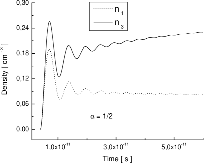
Figure 1: Time evolution of the particle number density with initial condition $m_{0}\cdot t_{0}=1$ for $\alpha=1/2$ (left) and the corresponding momentum distribution at the time $t\gg t_{0}$ (right).

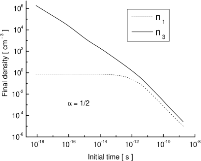
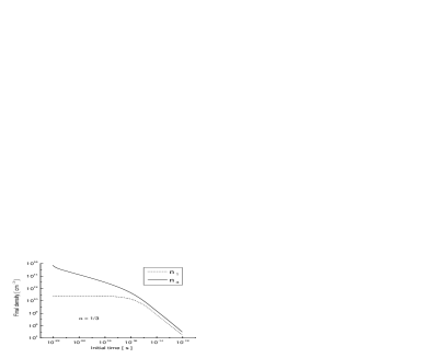
Figure 2: The dependence of the final particle number density on the initial time: $\alpha=1/2$ (left), $\alpha=1/3$ (right).

Due to back reactions and dynamical mass generation during the cosmic evolution the detailed mass history remains to be worked out. The central question, however, is whether the number density of produced W-bosons could be of the same order as that of the CMB photons, $n_{\rm CMB}\sim 465~{}{\rm cm}^{-3}$. If this question could be answered positively, the vacuum pair creation of W-bosons from a time-dependent scalar field (mass term) could be suggested as a mechanism for the generation of matter and radiation in the early Universe. The non-Abelian nature of the W-bosons could even imply consequences for the generation of the baryon (and lepton) asymmetry due to topological effects DB .

The numerical analysis of the Eqs. (50) is performed by a standard Runge-Kutta method on a one-dimensional momentum grid. As one can see from Fig. 1, the creation process ends very quickly and the particle density saturates at some final value. The momentum distribution of particles is formed also very early when $m(t)\approx m_{0}$ and frozen in such form so that later on for times $t\gg t_{0}$ most of the particles have very small momentum $p\ll m(t)$. The spectrum of created bosons is essentially non-equilibrium, hence we should continue further the analysis of relevant dissipative mechanisms and other observable manifestations of the non-equilibrium state (e.g., CMB photons; in this connection, see, for example, Komatsu ).

The other interesting feature of the mechanism of particle production considered above is the qualitatively different form of momentum distribution when compared to the creation in the electric field. As is known, the electric field generates the pairs with monotonic momentum distribution and $f(p=0)=max$ in the fermion case and with non-monotonic distribution and $f(p=0)=0$ in the boson case Grib94 . The creation mechanism connected with time-dependent effective mass modifies this situation to the contrary: the boson have a monotonic distribution (Fig. 1) and the fermions a non-monotonic one. The dependence of the corresponding final value of density on the initial time is shown in Fig. 2. The final density $n_{1}$ of particles with spin projection $\pm 1$ reaches a maximum, when we let the initial time go to very early times, close to the birth of the Universe. However, in the same limit, the density $f_{3}$ of particles with spin projection zero grows beyond all bounds. The choice of the EoS changes drastically the quantity of the created particles, thus giving values which are too small ($\alpha=1/2$) or too large ($\alpha=1/3$) in comparison with the observed CMB photon densities. In order to improve this model, we should use an improved EoS, assuming that the barotropic parameter $\gamma$ charcterizing the evolution of the particle masses can change during the time evolution. Such a time-dependence could be induced by the back-reaction of the created particles on the scalar field. Furthermore, we could use another space-time model, e.g., the Kasner space-time SmolHP instead of the conformally flat de Sitter one. The main achievement relative to the earlier work DB is that in the present approach, there is no divergence in the distribution function, thus we do not need to introduce some ambiguous regularization procedure.

V EOS for the isotropic case

The relations for the energy density and pressure can be obtained from the energy-momentum tensor corresponding to the Lagrangian (2)

$$T_{\mu\nu}=-\partial_{\mu}u^{*}_{\alpha}\partial_{\nu}u^{\alpha}-\partial_{\nu}u^{*}_{\alpha}\partial_{\mu}u^{\alpha}-g_{\mu\nu}\mathcal{L}.$$ (62)

Thus, we have $\varepsilon=\langle 0_{in}|T_{00}|0_{in}\rangle$ and $p=1/3\langle 0_{in}|T_{ii}|0_{in}\rangle$. Let us substitute the decompositions (5) and use the relations, which are a consequence of the spatial homogeneity of the system (in the discrete momentum representation)

$$\langle 0_{in}|a^{(+)}_{\mu}(\mathbf{p},t)a^{(-)}_{\nu}(\mathbf{p}^{\prime},t)|0_{in}\rangle = (2\pi)^{3}\delta_{\mathbf{p},\mathbf{p}^{\prime}}F_{\mu\nu}(\mathbf{p},t),$$

$$\langle 0_{in}|b^{(-)}_{\mu}(-\mathbf{p},t)b^{(+)}_{\nu}(-\mathbf{p}^{\prime},t)|0_{in}\rangle = (2\pi)^{3}\delta_{\mathbf{p},\mathbf{p}^{\prime}}\tilde{F}_{\mu\nu}(\mathbf{p},t),$$ (63)

$$\langle 0_{in}|a^{(\pm)}_{\mu}(\mathbf{p},t)b^{(\pm)}_{\nu}(-\mathbf{p}^{\prime},t)|0_{in}\rangle = (2\pi)^{3}\delta_{\mathbf{p},\mathbf{p}^{\prime}}F^{(\pm)}_{\mu\nu}(\mathbf{p},t).$$

As a result we obtain the following expressions for the energy density and the pressure (after the transition to the thermodynamic limit, $d\,\Gamma=(2\pi)^{-3}d^{3}p$)

$$\varepsilon(t) = -\int d\,\Gamma\,\omega(\mathbf{p},t)[F_{\mu}^{\mu}(\mathbf{p},t)+\tilde{F}_{\mu}^{\mu}(\mathbf{p},t)],$$ (64)

$$p(t) = \frac{1}{3}\int\frac{d\,\Gamma}{\omega(\mathbf{p},t)}\biggl{\{}-\mathbf{p}^{2}[F_{\mu}^{\mu}(\mathbf{p},t)+\tilde{F}_{\mu}^{\mu}(\mathbf{p},t)]$$ (65)

$$+ (2\mathbf{p}^{2}+3m^{2})[F_{\mu}^{(+)\mu}(\mathbf{p},t)+F_{\mu}^{(-)\mu}(\mathbf{p},t)]\biggr{\}}.$$

We perform now the series of the consecutive transformations of the functions $F_{\mu}^{\mu}(\mathbf{p},t)$, $\tilde{F}_{\mu}^{\mu}(\mathbf{p},t)$ and $F_{\mu}^{(\pm)\mu}(\mathbf{p},t)$: the exclusion of the $\mu=0$ component (according to Eq. (11)) and the transition to the complete QPR with the help of Eqs. (30). Thus, we arrive at

$$F_{\mu}^{\mu}(\mathbf{p},t)=-\sum_{l=1}^{3}f_{l}(\mathbf{p},t),\;\;\tilde{F}_{\mu}^{\mu}(\mathbf{p},t)=-\sum_{l=1}^{3}\tilde{f}_{l}(\mathbf{p},t),$$ (66)

$$F_{\mu}^{(\pm)\mu}(\mathbf{p},t)=-\sum_{l=1}^{3}f^{(\pm)}_{l}(\mathbf{p},t)-2\frac{p^{2}}{m^{2}}f_{3}^{(\pm)}(\mathbf{p},t),$$ (67)

where $f_{l}(\mathbf{p},t)$, $\tilde{f}_{l}(\mathbf{p},t)$ and $f^{(\pm)}(\mathbf{p},t)$ are the corresponding functions in the complete QPR. The substitution of these relations into Eqs. (64) and (65) leads to the following expressions for the energy density and pressure

$$\varepsilon(t) = 2\sum_{l=1}^{3}\int d\,\Gamma\omega(\mathbf{p},t)f_{l}(\mathbf{p},t),$$ (68)

$$p(t) = \frac{1}{3}\sum_{l=1}^{3}\int\frac{d\,\Gamma}{\omega(\mathbf{p},t)}\biggl{\{}2p^{2}f_{l}(\mathbf{p},t)-[2\omega^{2}(\mathbf{p},t)+m^{2}]$$ (69)

$$\times\left(\frac{2p^{2}}{3m^{2}}\left[f_{3}^{(+)}(\mathbf{p},t)+f_{3}^{(-)}(\mathbf{p},t)\right]+\left[f_{l}^{(+)}(\mathbf{p},t)+f_{l}^{(-)}(\mathbf{p},t)\right]\right)\biggr{\}}.$$

Taking into account the isotropy of the system, we obtain the EOS for the massive vector boson gas

$$\varepsilon(t) = 2\int d\,\Gamma\omega(2+Q)f_{1},$$ (70)

$$p(t) = \frac{2}{3}\int\frac{d\,\Gamma}{\omega}\left[2\mathbf{p}^{2}(2+Q)f_{1}\right]+\delta p_{vac}(t),$$ (71)

where $\delta p_{vac}(t)$ is the contribution in the pressure induced by the vacuum polarization,

$$\delta p_{vac}(t)=-\frac{2}{3}\int\frac{d\,\Gamma}{\omega}\,\biggl{(}2\omega^{2}+m^{2}\biggr{)}\left[1+Q\left(\frac{1}{2}+\frac{\mathbf{p}^{2}}{m^{2}}\right)\right]u_{1}.$$ (72)

In order to prove the convergence of the integrals (70) - (72) we investigate the asymptotic behavior of the solution to the system of Eqs. (50). This system can be solved exactly in the asymptotic limit $p\gg m$ for the case $\alpha=1/2$ when it gets the form

$$\dot{f} = \frac{m_{H}^{2}}{4t_{H}}\frac{1}{p^{2}}u,$$

$$\dot{u} = \frac{m_{H}^{2}}{2t_{H}}\frac{1}{p^{2}}(1+2f)-2pv,$$

$$\dot{v} = 2pu~{}.$$ (73)

The solution of (V) with the initial conditions (53) is

$$f(p,t) = \frac{\sin^{2}{p(t-t_{0})}}{16(p/m_{0})^{6}},$$

$$u(p,t) = \frac{1}{2}v(p,t)=\frac{\sin{2p(t-t_{0})}}{4(p/m_{0})^{3}},$$ (74)

where $m_{0}=m(t_{0})$. The numerical investigation of the general Eqs. (50) shows that the basic features of the solutions (V) for $\alpha=1/2$ are conserved also for other $\alpha>0$.

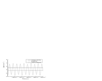
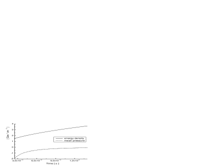
Figure 3: Time dependence of energy density and pressure at $t\gg t_{0}$ with initial condition $m_{i}\cdot t_{i}=1$ for $\alpha=1/2$.

According to (V), the particle and energy densities (Eqs. (55) and (70), respectively) are convergent, but the vacuum polarization contribution to the pressure (72) is divergent. Moreover, irrelevant fast vacuum oscillations of the pressure are observed here. Let us remark that such a behavior of the pressure for a plasma created from the is not a special feature of the present theory but is characteristic also for the models where an electron - positron plasma is created in strong, time-dependent electrodynamic fields as investigated in 23 . The standard regularization procedure of similar integrals with some unknown functions satisfying ordinary differential equations is based on the investigation of asymptotic decompositions of these functions in power series of the inverse momentum, $1/|\vec{p}|^{n}$ (the procedure of n-waves regularizations nw ). In the considered case, such a procedure is not effective because the solutions (V) has fastly oscillating factors (”zitterbewegung”), the asymptotic decompositions of which lead to the secular terms. Therefore we regularize the pressure by a momentum cut-off at $p=10m_{0}$ and separate its stable part by the time averaging

$$<p>=\frac{1}{(t-t_{0})}\int\limits_{t_{0}}^{t}p(t)dt.$$ (75)

The such ”coarse graining” procedure was proposed in 19 in order to exclude the ”zitterbewegung” from the description of vacuum particle creation. In reality, the smoothing of these fast oscillations occurs due to dissipative processes that are not taken into account here.

Fig. 3 shows that the mean pressure remains negative and its magnitude becomes negligible in comparison with the energy density. At large times the energy density grows but the pressure stays very small, $p\simeq 0$. The energy growth with the condition $p\simeq 0$ leads the conclusion mentioned in Sect. IV that the massive vector boson-anti-boson gas created from the vacuum is a cold one (see also Fig. 1). It can be seen directly from Eq. (70), that at large times $\epsilon(t)\simeq m(t)n(t)$, because of $\omega(t)\simeq m(t)$. Let us remark also that such an EoS of the massive vector boson gas ($\epsilon\neq 0$ and $p\simeq 0$) corresponds to dust-like matter 20 , which would characterize the evolution of the Universe during those stages when the vector boson gas is the dominant component of its matter/energy content. On the qualitative level, this conclusion is valid independent of the concrete choice of an EoS and, in particular, in the case of the dust-like EoS. In a subsequent work, we plan to obtain a formula of the type (61) as a result of the solution of the Friedman equation with the EoS (70)-(72) (such a procedure represents the back reaction problem) and to investigate self-consistently the production of vector bosons in the Universe.

VI Summary

The present work was devoted to the kinetic description of vacuum creation of massive vector bosons caused either by a time dependence of the mass or by the action of a non-stationary electric field. The statement of the problem is stimulated by modern cosmological problems related to the need for an explanation of the nature of the recently uncovered accelerating expansion of the Universe. The resulting KE (42) of non-Markovian type is obtained within a powerful non-perturbative framework and using the OR which provides an effective approach to the QPR, in the language of which the kinetic theory is constructed. We apply then this KE for the analysis of the important particular case of an isotropic gas of vector bosons with a time dependent mass which can be justified on the basis of a conformal-invariant scalar-tensor theory of gravitation. We show that the kinetic theory leads to a reasonable density of vector bosons in an early period of the Universe evolution which is sufficient to explanation the present density of CMB photons.

The obtained results constitute a foundation for the subsequent investigation of the dynamics of vector bosons created from the vacuum (the equation of state, the long wave-length acoustic excitations, the back-reaction problem etc.). It is necessary to underline that we have considered here the single mechanism of mass change induced by the conformal expansion of the Universe. It was necessary to switch on the mass $m_{0}(t_{0})$ at some arbitrary initial time $t_{0}$. Thus, for the construction of a more consistent theory, one should eventually take into account the inflation mechanism of mass generation acting during an earlier period the Universe evolution 18 ; 22 ; 24 ; 25 .

It is very interesting to investigate the generation of elementary particles of different masses. Eq. (61) is valid for all elementary particles independent of their inner symmetry class. Then the chemical composition of created matter and the EoS of the Universe must be fixed rather precisely and can be subject to experimental verification.

Acknowledgement

This work was partly supported by a Russian Federations State Committee for Higher Education grant No. E02-3.3-210 and RFBR grant No. 03-02-16877. S.A.S. acknowledges by DFG grant No. 436 RUS 117/78/04, D.B. was supported by the Virtual Institute of the Helmholtz association under grant No. VH-VI-041. We are grateful to Prof. M.P. Da̧browski for discussion of some cosmological aspects of the present work.

References

• (1) A.I. Nikishov, JETP 93, 197 (2001).
• (2) A.A. Grib, S.G. Mamaev and V.M. Mostepanenko, Vacuum Quantum Effects in Strong External Fields, (Friedmann Laboratory Publishing, St. Peterburg, 1994).
• (3) H.-P. Pavel and V.N. Pervushin, Int. J. Mod. Phys. A 14, 2285 (1999).
• (4) V.S. Vanyashin and M.V. Terentyev, Zh. Eksp. Teor. Fiz. 48, 565 (1965).
• (5) M.S. Marinov and V.S. Popov, Yad. Fiz. 15, 1271 (1972).
• (6) V.M. Mostepanenko, F.M. Frolov, and V.A. Sheliuto, Yad. Fiz. 37, 1261 (1983).
• (7) S.I. Kruglov, Int. J. Theor. Phys. 40, 515 (2001).
• (8) D. Blaschke, V.N. Pervushin, D.V. Proskurin, S.I. Vinitsky, and A.A. Gusev, Phys. of Atomic Nucl. 67, 1050 (2004).
• (9) A.A. Grib and A.V. Nesteruk, Yad. Fiz. 35, 216 (1982).
• (10) V.V. Skalozub, Yad. Fiz. 21, 1337 (1975); 31, 1980 (1980).
• (11) E. L. Bratkovskaya, W. Cassing, R. Rapp and J. Wambach, Nucl. Phys. A 634, 168 (1998), and references therein.
• (12) S.M. Schmidt, D. Blaschke, G. Röpke, S.A. Smolyansky, A.V. Prozorkevich, and V.D. Toneev, Int. J. Mod. Phys. E 7, 709 (1998).
• (13) V.N. Pervushin, V.V. Skokov, A.V. Reichel, S.A. Smolyansky, and A. V. Prozorkevich, Int J. Mod. Phys. A (in press); hep-ph/0307200.
• (14) V.N. Pervushin, D.V. Proskurin, and A.A. Gusev, Grav. Cosmology 8, 181 (2002).
• (15) Ya.B. Zeldovich, JETP 41, 1609 (1961)
• (16) S.A. Smolyansky, A.V. Reichel, D.V. Vinnik, and S.M. Schmidt, in Progress in Nonequilibrium Green’s Functions II, M. Bonitz and D. Semkat (eds.), (World Scientific, Singapore, 2003), p. 384.
• (17) C. Itzykson and J.B. Zuber, Quantum Field Theory, (McGraw-Hill, 1980);
N.N. Bogoliubov and D.V. Shirkov, Introduction to the Theory of Quantized Fields, 3rd ed. (Wiley, 1980).
• (18) S. Schmidt, D. Blaschke, G. Röpke, A.V. Prozorkevich, S.A. Smolyansky, and V.D. Toneev, Phys. Rev. D 59, 094005 (1999).
• (19) A. Dolgov, in Multiple Facets of Quantization and Supersymmetry, M. Olshavetsky, and A. Vainshtein (eds.), (World Scientific, Singapore, 2002), p. 104.
• (20) D.V. Vinnik, V.A. Mizerny, V.A. Prozorkevich, S.A. Smolyansky, and V.D. Toneev, Yad. Fiz. 64, 836 (2001).
• (21) D. Blaschke and M.P. Da̧browski, hep-th/0407078.
• (22) E. Komatsu and D.N. Spergel, Phys.Rev. D63, 063002 (2001); F. Vernizzi, A. Melchiorri, and R. Durrer, Phys. Rev. D63, 063501 (2001).
• (23) S.A. Smolyansky, A.V. Prozorkevich, D.V. Vinnik, and A.V. Reichel, Proc. of Int. Workshop ”Hot point in Astrophysics”, Dubna, 2000, p.364.
• (24) S.G. Mamaev and N.N. Trunov, Yad. Phys. 30, 1302 (1979) (in russian).
• (25) Ya.B. Zeldovich and A.A. Starobinsky, Sov. Phys. JETP, 34, 1159 (1971).
• (26) J. Rau and B. Müller, Phys. Rep. 272, 1 (1996).
• (27) M.P. Dabrowski and J. Stelmach, Ap. J. 97, 978 (1989).
• (28) J.A. Casas, J.Garcia-Bellido and M. Quiros, Class. Quant. Grav., 9, 1371 (1992); G.W. Anderson and S.M. Carroll, astro-ph/9711288.
• (29) P.B. Green and L. Kofman, Phys.Lett. B, 448), 6 (1999).
• (30) Proceedings of the 18-th IAP Astrophys. Colloquium “On the Nature of Dark Energy”, Jul 1-5 (2002), Eds: Ph. Brax, J. Martin, J.-Ph. Uzan (Frontier Group, Paris, 2002).
• (31) L. Parker, Phys. Rev. Lett. 21, 562 (1968); Phys Rev. 183, 1057 (1969); ibid, D3, 346 (1971); Phys. Rev. Lett. 28, 705 (1972); Phys. Rev. D7, 976 (1973).
• (32) A.A. Grib and S.G. Mamaev, Yad. Fiz. 10, 1276 (1969).
• (33) R.U. Sexl and H.K. Urbantke, Phys. Rev. 179, 1247 (1969).
• (34) Ya.B. Zeldovich, Pisma Zh. Exp. Teor. Fiz. 12, 443 (1970); Ya.B. Zeldovich and A.A. Starobinsky, Zh. Exp. Teor. Fiz. 61, 2161 (1971).
• (35) N.D. Birrell, P.C.W. Davies, Quantum Fields in Curved Spaces, (Cambridge Univ. Press, Cambridge, 1982).
• (36) Ya.B. Zeldovich and I.D. Novikov, Structure and Evolution of the Universe, (Univ. Chicago Press, Chicago, 1983).
• (37) Y. Fujii, K.-I. Maeda, The Scalar-Tensor Theory of Gravitation, (Cambrige Univ. Press, Cambridge, 2003).