Factorization of Large-$x$ Quark Distributions in a Hadron

Abstract

We present a factorization formula for valence quark distributions in a hadron in $x\rightarrow 1$ limit. For the example of pion, we arrive at the form of factorization by analyzing momentum flow in the leading and high-order Feynman diagrams. The result confirms the well-known $1-x$ scaling rule to all orders in perturbation theory, providing the non-perturbative matrix elements for the infrared-divergence factors. We comment on re-summation of perturbative single and double logarithms in $1-x$.

Three decades ago, Brodsky, Farrar and others made a perturbative quantum chromodyanmics (pQCD) prediction about the power behavior of parton distributions as $x\rightarrow 1$, i.e., the density of quarks carrying almost all the longitudinal (plus) momentum of a hadron participating in hard scattering Gunion:1973nm ; Blankenbecler:1974tm ; Farrar:1975yb ; Lepage:1980fj . Through calculating the leading pQCD diagrams, they showed that the valence quark distribution goes like, for example, $(1-x)^{2}$ in the pion and $(1-x)^{3}$ in the nucleon. The basic argument is that when the valence quark carries nearly all the plus momentum, the relevant QCD configurations in hadron wave functions must be far off-shell and hence are amenable to pQCD treatment. The result has since been generalized to the sea quarks, gluons, helicity-dependent distributions Brodsky:1994kg , and lately to generalized parton distributions Yuan:2003fs . The above power law is consistent with the large-momentum behavior of the elastic form factors through the so-called Drell-Yan-West relation Drell:1969km ; West:1976tn ; Melnitchouk:2001eh .

Despite its elegance and usefulness, a rigorous derivation of the scaling rule in pQCD has not, to the authors’ knowledge, been established in the literature. Indeed, if one follows the original calculations, the scaling term has a power-like infrared-divergent coefficient $\int{d^{2}k_{\perp}}/{(k_{\perp}^{2})^{2}}$ for the pion, and similarly for the nucleon. One might argue that this divergence will be tamed by non-perturbative QCD effects and hence does not affect power counting. A more satisfactory solution, however, is to formulate a factorization theorem explicitly separating the long distance contributions from short distance ones. QCD factorization will establish the scaling rule through a systematic QCD power counting, and hence validate the result to all orders in perturbation theory. It will also provide well-defined non-perturbative matrix elements to absorb infrared divergences. Finally, factorization will provide a convenient tool to re-sum possible large Sudakov double logarithms present in $x\rightarrow 1$ limit.

The goal of this paper is to establish a factorization formula for the valence quark distributions in a hadron in the large-$x$ limit. We consider the example of a pion, although similar studies apply to other hadrons such as the nucleon. The factorization arises from a detailed analysis of momentum flow in the lowest-order pQCD diagrams and their generalization to all orders. Without an explicit calculation, an infrared power counting allows a straightforward determination of the $1-x$ power behavior. The factorized expression contains hard parts, initial and final state jets, and a soft function, as easily seen from the leading $1-x$ structure of reduced diagrams. We introduce a non-perturbative matrix element for the soft factor which absorbs the perturbative infrared divergence mentioned earlier.

The large-$x$ behavior of the valence quark distributions in a pion was obtained from calculating the lowest-order Feynman diagrams, one of which is reproduced in Fig. 1a. Let us choose the light-cone system of coordinates defined by two light-cone vectors $p^{\mu}=\Lambda(1,0,0,1)$ and $n^{\mu}=(1,0,0,-1)/(2\Lambda)$ ($p^{2}=n^{2}=0$, $p\cdot n=1$). Any vector $k^{\mu}$ can be expanded in terms of $p^{\mu}$ and $n^{\mu}$, as $k^{\mu}=k\cdot np^{\mu}+k\cdot pn^{\mu}+k_{\perp}^{\mu}$. We choose the pion momentum mainly along the $p$-direction ($p^{+}$ taken as large), $P^{\mu}=p^{\mu}+m_{\pi}^{2}/2n^{\mu}$, ignoring the $m_{\pi}^{2}$-term except when it is needed to regularize infrared divergences. As labelled in the figure, the incoming quark carries momentum $x_{1}p^{\mu}$ and anti-quark momentum $(1-x_{1})p^{\mu}\equiv\bar{x}_{1}p^{\mu}$. The anti-quark going through the final state cut (shown by the dashed line) has momentum $k^{\mu}$ integrated over.

Instead of doing an explicit calculation to reproduce the familiar result $q(x)\sim f_{\pi}^{2}(1-x)^{2}\int d^{2}k_{\perp}/(k_{\perp}^{2})^{2}$, let us analyze the momentum flow of the loop integral over $k^{\mu}$. In the $x\rightarrow 1$ limit, the $p$ (or plus) component of $k$ is constrained to $(1-x)p$ and is soft, $\sim\lambda$. If the transverse momentum $k_{\perp}$ is on the order of $(1-x)^{1/2}p^{+}$, the $n$ component of $k$ must be very large, $k^{-}=k_{\perp}^{2}/2(1-x)p^{+}\sim p^{+}$. Then the anti-quark line is jet-like, and going along the $n$-direction. The corresponding reduced diagram is shown in Fig. 1b. If, on the other hand, $k_{\perp}$ is soft $(1-x)p^{+}$, $k^{-}$ also remains soft. The anti-quark line is now a soft line. The corresponding reduced diagram is shown in Fig. 1c. Using an infrared power counting generalizable to all orders in perturbation theory, one can obtain $q(x)\sim(1-x)^{2}$. We refer the reader to well-known references for the details of infrared power counting stermanbook ; CSS89 .

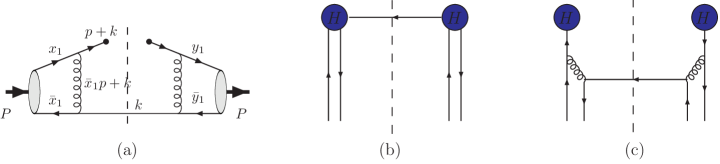
Figure 1: a). A lowest-order Feynman diagram contributing to the leading-$1-x$ power of valence quark distribution in a pion. b). A reduced diagram in which the final state anti-quark is a jet along the $n$-direction. c). An alternative reduced diagram in which the final state anti-quark is soft.

If the anti-quark is collinear to the $n$-direction (Fig.1b), the infrared power of the diagram is $0$, obtained from the final-state quark line as a jet, $\int d^{4}k\delta(k^{2})\delta(k^{+}-(1-x)p^{+})$. The polarization sum of the final-state quark is proportional to $k^{-}\sim p^{+}$ and hence does not contribute any soft power. However, an explicit calculation also finds a factor $k_{\perp}^{2}$ in the hard part. This suppression factor is not included in ordinary power counting, and is resulting from the spin structure of the diagram. Taking into account this additional contribution, the actual infrared scaling of Fig. 1b is $\lambda$. Infrared factors of a Feynman diagram come from both $1-x$ and transverse momentum. The dimensionless quark distribution is proportional to $f_{\pi}^{2}$ from the pion wave function. Thus the transverse-momentum integral must be proportional to $f_{\pi}^{2}\int{d^{2}k_{\perp}}/{(k_{\perp}^{2})^{2}}$. Hence, the quark distribution has $(1-x)$-related infrared power $2$, or is proportional to $(1-x)^{2}$. The same counting applies to all other leading-order diagrams which are not shown explicitly.

When the final-state quark is soft, the gluon and internal quark lines become collinear to the pion momentum (Fig.1c). The denominators in the pion jets contribute $\lambda^{-4}$. Two collinear-quark-gluon couplings contribute soft-power $\lambda^{2}$: Usually a coupling contributed by a collinear transverse-momentum $k_{\perp}$ is counted as $\lambda^{1/2}$. In the present case, however, the transverse momentum in the pion jets originates from the soft quark and thus must be treated as the soft scale $\lambda$. The final-state soft quark contributes $\lambda^{2}$. So the total soft power is $0$. After factoring the transverse-momentum integral, one has a $(1-x)$-related soft-power 2, or the pion distribution goes like $(1-x)^{2}$, just like in the first region, Fig. 1b.

The above consideration and result are generic. For a general Feynman diagram of an arbitrary order contributing to parton distributions at $x\rightarrow 1$, the momentum integrations contain many different regions (pinched surfaces) stermanbook ; CSS89 , each of which can be represented by a product of the various parts: the two incoming jets along the $p$-direction ($J_{L,R}$), the out-going jets along the $n$-direction ($J_{\beta}$), and two hard parts ($H_{L,R}$), each on the different sides of the cuts connecting the $p$ and $n$ jets, and finally a soft part connecting all jets and hard parts, as shown in Fig. 2a. Similar factorization for the quark distribution in a quark has been considered in Sterman:1986aj ; Korchemsky:1988si ; Berger:2002sv

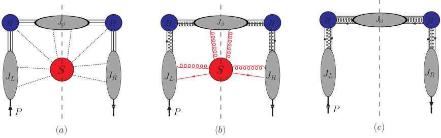
Figure 2: a). A general reduced diagram for parton distributions at $x\rightarrow 1$. b). A leading region where the anti-quark goes through the soft part and the final state jet containing the eikonal line and longitudinally polarized gluons. b). Another leading region where the anti-quark is part of the final-state jet. There is no soft factor here because the initial and final state jets are all color neutral.

Let us use $p_{J}$ to denote the number of collinear quarks or gluons with-physical-polarization lines entering the hard part from jet $J$; use $l_{j}$ to represent the number of collinear gluons of longitudinal polarization through a similar attachment; use $E_{J}^{b,f}$ to denote the number of soft bosons or fermions connecting to the left or right hard part; use $E^{b,f}_{HL,R}$ to label the number of soft bosons of fermions connecting to the left or right hard part; and finally use $v_{J}^{3}$ to label the number of three-point vertices in the jet, and $s_{J}$ the number of soft gluons with scalar polarization and soft quarks attaching to the jet. Then the soft part has infrared power,

$$\omega_{S} = E^{b}_{J,L}+E^{b}_{J,R}+E^{b}_{J,\beta}+E^{b}_{HL}+E^{b}_{HR}$$ (1)

$$+\frac{3}{2}\left(E^{b}_{J,L}+E^{b}_{J,R}+E^{b}_{J,\beta}+E^{b}_{HL}+E^{b}_{HR}\right)\ .$$

On the other hand, the infrared power associated with each jet is

$$\omega_{J}=\frac{1}{2}(p_{J}-s_{J}-E_{J}^{b}-E^{f}_{J}-I_{J})+\frac{1}{2}\left(s_{J}+l_{J}-v^{(3)}\right)\theta\left(s_{J}+l_{J}-v^{(3)}\right)\ .$$ (2)

Combining the above results, one finds

$$\omega(G) \geq \frac{1}{2}\left(p_{J_{L}}+p_{J_{R}}+p_{J_{\beta}}\right)-2-\frac{1}{2}(I_{J_{L}}+I_{J_{R}})$$ (3)

$$+\frac{1}{2}\left(E^{b}_{J_{L}}+E^{b}_{J_{R}}+E^{b}_{J_{\beta}}\right)-\frac{1}{2}\left(s_{J_{L}}+s_{J_{R}}+s_{J_{\beta}}\right)$$

$$+E^{f}_{J_{L}}+E^{f}_{J_{R}}+E^{f}_{\beta}+E^{b}_{HL}+E^{b}_{HR}+\frac{3}{2}(E^{f}_{HL}+E^{f}_{HR})$$

$$+\frac{1}{2}\left(s_{J_{L}}+l_{J_{L}}-v_{J_{L}}^{(3)}\right)\theta\left(s_{J_{L}}+l_{J_{L}}-v_{J_{L}}^{(3)}\right)$$

$$+\frac{1}{2}\left(s_{J_{R}}+l_{J_{R}}-v_{J_{R}}^{(3)}\right)\theta\left(s_{J_{R}}+l_{J_{R}}-v_{J_{R}}^{(3)}\right)$$

$$+\frac{1}{2}\left(s_{J_{\beta}}+l_{J_{\beta}}-v_{J_{\beta}}^{(3)}\right)\theta\left(s_{J_{\beta}}+l_{J_{\beta}}-v_{J_{\beta}}^{(3)}\right)\ .$$

where we have taken into account the constraint that the plus momentum going through the final state cut is $(1-x)p\sim\lambda$, and the eikonal line is accounted for by $p_{J_{\beta}}=2$. The above result generalizes that for a single quark state Berger:2002sv .

For a pion, $I_{J_{L}}=I_{J_{R}}=2$, and the lowest infrared power is $-1$, obtained when $p_{J_{L,R}}=1$, $p_{J_{\beta}}=2$, $E^{f}_{J_{L}}=E^{f}_{J_{R}}=1$, $E^{f}_{\beta}=0$, $s_{J_{\beta}}=E^{b}_{\beta}$, and $s_{J_{L,R}}=E^{b}_{J_{L,R}}+1$. The corresponding reduced diagram is shown in Fig. 2b, where the final-state jet contains just the eikonal line and longitudinally-polarized gluons, and the soft part contains an anti-quark line. The jets going into the hard parts contain a single quark and an arbitrary number of longitudinally polarized gluons. We argue, however, that the actual infrared power is 0 when taking into account an additional numerator suppression, just as in the leading-order diagram in Fig. 1. Observe that the infrared power of an initial-state jet is always an half-integer, which means the jet is proportional to at least one transverse momentum, even after all integrals in the jet are carried out. However, the only relevant transverse momenta available are those of the soft lines. Therefore, this transverse momentum must be counted as $\lambda$, not $\lambda^{1/2}$. With this extra suppression, the actual infrared power of the reduced diagram in Fig. 2b is 0. Factorizing out the transverse-momentum integral, one gets $q(x)\sim(1-x)^{2}$ to all orders in perturbation theory.

The next lowest infrared power, 0, is obtained when $p_{J_{R}}=p_{J_{R}}=2$, $p_{J_{\beta}}=4$, all $E^{f}=0$ and $E^{b}_{H}=0$, and $E^{b}_{J}=s_{J}$. The corresponding reduced diagram is shown in Fig. 2c, where the final-state jet has an anti-quark quantum number. The soft-gluon radiation is not drawn because the initial and final state jets are color-neutral; and thus when summing over all final states, the soft factor reduces to 1, i.e., the soft radiation must cancel. Because of the angular momentum conservation, there is a numerator suppression factor proportional to the transverse-momentum $k_{\perp}^{2}$ of the anti-quark jet, as seen in Fig. 1a. The argument goes as follows. Consider deep-inelastic scattering on a pion target. If the final state consists of two collinear quark-antiquark jets plus an arbitrary number of longitudinally polarized gluons going exactly along the $n$ direction, the scattering amplitude vanishes identically. This is because when the initial and final states are collinear and with zero helicity (fermion helicity is conserved in gauge theory), scattering with a physical photon of helicity $\pm 1$ is forbidden by angular momentum conservation. Therefore, there must be a relative transverse-momentum between the quark and anti-quark jets, $k_{\perp}^{2}\sim(1-x)Q^{2}$. The scattering amplitude is proportional to $k_{\perp}$, and the parton distribution is proportional to $k_{\perp}^{2}$. The actual infrared factor is then $\lambda$. Accounting for the transverse-momentum integral, one again gets a scaling law $(1-x)^{2}$ to all orders in perturbation theory.

One can write down a factorization formula for the two reduced diagrams shown in diagrams 2b and 2c, after factorizing the collinear longitudinally polarized gluons from the hard parts and the soft gluons from the initial state jets. For example, let us consider the case when the anti-quark is soft (Fig. 2b). Going through steps similar to those outlined in CSS89 ; Berger:2002sv , one finds

$$q_{\pi}(x\rightarrow 1) = H_{L}(p,\mu)H_{R}(p,\mu)\tilde{J}_{p,L}(p,\mu)\tilde{J}_{p,R}(p,\mu)$$ (4)

$$\times\sum_{C_{\beta},C_{S}}\prod_{m_{L},m_{R},l}\int\frac{d^{n}q_{L,m_{L}}}{(2\pi)^{n}}\frac{d^{n}q_{R,m_{R}}}{(2\pi)^{n}}\frac{d^{n}q_{l}}{(2\pi)^{n}}$$

$$\times{\cal E}_{L}(p,\{q_{L,m_{L}}\})^{\{\gamma_{m_{L}}\}}{\cal E}_{R}(p,\{q_{R,m_{R}}\})^{\{\gamma_{m_{R}}\}}$$

$$\times\int dy\int dzS^{(C_{S})}\left(yp,\mu;\{q_{L,m_{L}}^{\gamma_{m_{L}}}\};\{q_{R,m_{R}}^{\gamma_{m_{R}}}\};\{q_{l}^{\delta}\}\right)\tilde{J}_{\beta}^{(C_{\beta})}(zp,\mu;n;\{q_{l}^{\delta}\})$$

$$\times\delta^{n}\left(\sum_{m_{L}}q^{\mu}_{L,m_{L}}+\sum_{m_{R}}q^{\mu}_{R,m_{R}}+\sum_{l}q_{l}^{\mu}\right)\delta(1-x-y-z)\ ,$$

where $H_{L,R}$ represent the hard contributions with collinear longitudinally-polarized gluons factorized, $\tilde{J}_{L,R}$ represent the jet contributions with soft gluons and quarks factorized. The factorized soft gluons are now represented by the two eikonal lines ${\cal E}_{L,R}$. The soft loop momenta to be integrated over connect the soft part and the eikonal lines, the soft part and final-state jets. The summations are over all possible cuts through final-state jet $C_{\beta}$ and soft part $C_{S}$. The longitudinal momenta going through the final state cuts are constrained by $1-x$. The soft function and jets can be represented by non-perturbative QCD matrix elements.

One can define the gauge-invariant quark-eikonal cross section,

$$\sigma^{\rm eik}((1-x)p,\mu)=\frac{1}{N_{c}}\int\frac{dy^{-}}{2\pi}e^{i(1-x)p^{+}y^{-}}\sum_{n,a}\langle 0|\overline{\Psi}_{a}(y^{-})|n\rangle\gamma^{+}\langle n|\Psi_{a}(0)|0\rangle\ ,$$ (5)

where $\Psi(y^{-})$ is defined as

$$\Psi(y^{-})=\int^{0}_{-\infty}dy^{+}U_{n}(\infty;y^{-})U_{P}(0^{+},y^{-};y^{+},y^{-})\psi(y^{+},y^{-})\ ,$$ (6)

with $U_{n}(\infty;y^{-})={\cal P}\exp\left(-ig\int^{\infty}_{y^{-}}d\lambda n\cdot A(\lambda n)\right)$, etc., and $P$ in $U_{P}$ is the pion momentum. $\sigma^{\rm eik}$ has a similar factorization as the parton distribution, except the pion jets are replaced by eikonal jets. Therefore, $x\rightarrow 1$ quark distribution can be expressed as,

$$q(x)=H_{L}(p,\mu)H_{R}(p,\mu)J_{L}(p,\mu)J_{R}(p,\mu)\sigma^{\rm eik}((1-x)p,\mu)\ .$$ (7)

The entire $x$-dependence can now be found from the quark-eikonal cross section. This result is very similar to the factorization of the quark distribution in a single quark in the same limit Korchemsky:1988si ; Korchemsky:1992xv ; Berger:2002sv . It is easy to check that at tree level, one reproduces the result from Fig. 1.

Apart from the simple power behavior considered so far, perturbative calculations also generate single and double logarithmic dependence in $1-x$. The single logarithmic dependence can be summed to yield a power correction $(1-x)^{A(\mu)}$, where $A(\mu)$ is renormalization-scale $\mu$ dependent Korchemsky:1988si . The evolution in $\mu$ can be calculated in perturbation theory, and the absolute magnitude of $A(\mu)$ can only be determined through non-perturbative methods. Soft-gluon radiations from charged lines produce large double logarithmic corrections of type $\alpha_{s}^{n}\ln^{m}(1-x)$ with $m\leq 2n-1$ BroLep80 ; Mueller:1981sg ; Sterman:1986aj ; Catani:1989ne ; Manohar:2003vb . These corrections depend on a precise definition of the parton distribution Sterman:1986aj and infrared regularizations. These issues will be discussed in a forth-coming publication.

To summarize, we have presented a factorization formula for the valence quark distribution in the pion valid to the leading power in $(1-x)$ and to all orders in perturbation theory. Through infrared power counting, one obtains the power dependence in $(1-x)$. The factorization theorem, however, allows one to calculate the coefficients of the power law non-perturbatively. It also allows one to re-sum large Sudakov double logarithms associated with soft radiations.

We thank G. Sterman for useful discussions. X. J. is supported by the U. S. Department of Energy via grant DE-FG02-93ER-40762, and F. Y. by the RIKEN-BNL Research Center. J.P.M. was supported by National Natural Science Foundation of P.R. China (NSFC). X. J. is also supported by a grant from NSFC.

References

- (1) J. F. Gunion, Phys. Rev. D 10, 242 (1974).
- (2) R. Blankenbecler and S. J. Brodsky, Phys. Rev. D 10, 2973 (1974).
- (3) G. R. Farrar and D. R. Jackson, Phys. Rev. Lett. 35, 1416 (1975).
- (4) G. P. Lepage and S. J. Brodsky, Phys. Rev. D 22, 2157 (1980).
- (5) S. J. Brodsky, M. Burkardt and I. Schmidt, Nucl. Phys. B 441, 197 (1995) [arXiv:hep-ph/9401328].
- (6) F. Yuan, Phys. Rev. D 69, 051501 (2004) [arXiv:hep-ph/0311288].
- (7) S. D. Drell and T. M. Yan, Phys. Rev. Lett. 24, 181 (1970).
- (8) G. B. West, Phys. Rev. D 14, 732 (1976).
- (9) W. Melnitchouk, Phys. Rev. Lett. 86, 35 (2001) [Erratum-ibid. 93, 199901 (2004)] [arXiv:hep-ph/0106073].
- (10) G. Sterman, An Introduction to Quantum Field Theory, Cambridge Univ. Press (1993).
- (11) J. C. Collins, D. E. Soper and G. Sterman, Adv. Ser. Direct. High Energy Phys. 5, 1 (1988); in Perturbative QCD, A.H. Mueller, ed. (World Scientific Publ., 1989).
- (12) G. Sterman, Nucl. Phys. B 281, 310 (1987).
- (13) G. P. Korchemsky, Mod. Phys. Lett. A 4, 1257 (1989).
- (14) C. F. Berger, Phys. Rev. D 66, 116002 (2002) [arXiv:hep-ph/0209107].
- (15) G. P. Korchemsky and G. Marchesini, Nucl. Phys. B 406, 225 (1993) [arXiv:hep-ph/9210281].
- (16) G. P. Lepage and S. J. Brodsky, Phys. Rev. D 22, 2157 (1980).
- (17) A. H. Mueller, Phys. Rept. 73, 237 (1981).
- (18) S. Catani and L. Trentadue, Nucl. Phys. B 327, 323 (1989).
- (19) A. V. Manohar, Phys. Rev. D 68, 114019 (2003) [arXiv:hep-ph/0309176].