Confronting next-leading BFKL kernels with proton structure function data

Abstract

We propose a phenomenological study of the Balitsky-Fadin-Kuraev-Lipatov (BFKL) approach applied to the data on the proton structure function $F_{2}$ measured at HERA in the small-$x_{Bj}$ region. In a first part we use a simplified “effective kernel” approximation leading to few-parameter fits of $F_{2}.$ It allows for a comparison between leading-logs (LO) and next-to-leading logs (NLO) BFKL approaches in the saddle-point approximation, using known resummed NLO-BFKL kernels. The NLO fits give a qualitatively satisfactory account of the running coupling constant effect but quantitatively the $\chi^{2}$ remains sizeably higher than the LO fit at fixed coupling. In a second part, a comparison of theory and data through a detailed analysis in Mellin space $x_{Bj}\to\omega,$ leads to a more model independent approach to the resummed NLO-BFKL kernels we consider and points out some necessary improvements of the extrapolation at higher orders.

I Introduction

Precise phenomenological tests of QCD evolution equations are one of the main goals of deep inelastic scattering phenomenology. For the Dokshitzer-Gribov-Lipatov-Altarelli-Parisi (DGLAP) evolution in $Q^{2}$ dglap , it has been possible to test it in various ways with NLO (next-to-leading $\log Q^{2}$) and now NNLO accuracy and it works quite well in a large range of $Q^{2}$ and $x_{Bj}.$ Testing precisely the Balitsky-Fadin-Kuraev-Lipatov (BFKL) evolution in energy bfkl (or $x_{Bj}$) beyond leading order appears more difficult. A theoretically convenient way would be to stay within the perturbative regime by using only massive or highly virtual colliding particles, but precision QCD phenomenology for the present day is provided mainly by the data data on deep-inelastic scattering at small $x_{Bj}.$

Indeed, the first experimental results from HERA confirmed the existence of a strong rise of the proton structure function $F_{2}$ with energy which, in the BFKL framework, can be well described by a simple (3 parameters) LO-BFKL fit old ; machado . The main issue of Ref.old was that not only the rise with energy but also the scaling violations observed at small ${x_{Bj}}$ are encoded in the BFKL framework through the $Q^{2}$ variation of the effective anomalous dimension. However one was led old to introduce an effective but unphysical value of the strong coupling constant

$\alpha\sim.07-.09$ instead of $\alpha\sim.2$ in the $Q^{2}$-range considered for HERA small-${x_{Bj}}$ physics, revealing the need for NLO corrections. Indeed, the running of the strong coupling constant is not taken into account.

In fact, the theoretical task of computing these corrections appears to be quite hard. It is now in good progress but still under completion. For the BFKL kernel, they have been calculated after much efforts next . In fact, they appeared to be so large that they miss by a large amount the phenomelogical requirements and could even invalidate the whole theoretical approach. Soon after, it was realized salam that the main problem comes from the existence of spurious singularities brought together with the NLO corrections, which ought to be cancelled by an appropriate resummation at all orders of the perturbative expansion, resummation required by consistency with the QCD renormalization group.

Indeed, various resummation schemes have been proposed salam ; autres ; lipatov which satisfy the renormalization group requirements while retaining the computed value of the NLO terms in the BFKL kernel. Hence, the constraints can be satisfied and the next-to-leading order introduced without compromising the theoretical consistency of the BFKL scheme. However, the situation remains not so clear concerning phenomenology.

To summarize the theoretical problems still remaining to be solved, the determination of the impact factors associated with the coupling of the NLO-BFKL kernels with the virtual photon are still in progress bartels . The factorization of the non perturbative coupling is also problematic at NLO-BFKL level. Another source of indeterminacy comes from instabilities at large energy of the evolution equations which may lead to the dominance of the non-perturbative “Pomeron” singularity instabilities .

On a phenomenological ground, we note that the resummation schemes possess some ambiguity, since higher order logs (beyond the next-to-leading ones) are not known, apart from the renormalization group constraints. Such variations appear, e.g. in Ref. salam , where first resummation schemes have been proposed. In practice, we will consider the schemes $S3$ and $S4$ of Ref. salam together with the one of Ref. autres , in the formulation of Ref. trianta , including quark contributions to the kernel.

The aim of our paper is to compare the phenomenological efficiency of LO versus NLO BFKL approaches using present precise experimental data on the proton structure function $F_{2}$. On the same footing it is also to compare phenomenologically the different NLO schemes in order to check their validity and distinguish between different resummation options for the NLO-BFKL kernels.

For this sake, we shall use a two-step approach. First, we will consider a simpler version of the NLO-BFKL formulae by considering an “effective kernel” obtained using a well-known “consistency condition” autres satisfied by the NLO-BFKL kernels. Then, we formulate a saddle-point approximation for both cases allowing a similar formulation for LO and NLO kernels.

Our study is organized as follows. In Sec.II, we present the construction of the effective kernels at LO and NLO levels and the corresponding saddle point approximation for the proton structure function $F_{2}$. In Sec.III, we use these formulations to perform fits to the structure function data in the range ($x_{Bj}\leq.01$ , $Q^{2}\leq 150\ GeV^{2}$) suitable for a BFKL analysis. In Section IV we perform a phenomenological determination of the Mellin transform $\tilde{F}_{2}(\omega,Q^{2})$ in the relevant range and, with this information, we discuss the “consistency condition” for the NLO-kernels under study. The final Section V is devoted to a summary, a discussion of our approximations and an outlook. An Appendix recalls the necessary formulae and definitions of the NLO kernels considered in this work.

II “Effective kernel” and saddle-point approximation of BFKL amplitudes

The BFKL formulation of the proton structure functions can be formulated in terms of the double inverse Mellin integral

$${F_{2}}=\int\!\int\frac{d\gamma d\omega}{(2i\pi)^{2}}\left(\frac{Q^{2}}{Q_{0}^{2}}\right)^{\gamma}{x_{Bj}}^{-\omega}\ {{\cal F}_{2}}(\gamma,\omega)\ .$$ (1)

At LO level one has (see, e.g. old )

$${{\cal F}_{2}}(\gamma,\omega)=\frac{h_{2}(\gamma,\omega)}{\omega-\bar{\alpha}\ \chi_{L0}(\gamma)}$$ (2)

where $\bar{\alpha}\equiv{\alpha_{s}N_{c}}/{\pi},$ $\alpha_{s}$ is the coupling constant which is merely a parameter at this LO level. The LO BFKL kernel is written as

$$\chi_{LO}(\gamma)=2\psi(1)-\psi(\gamma)-\psi(1-\gamma)\ .$$ (3)

$h_{2}(\gamma,\omega)$ is a prefactor which takes into account both the phenomenological non-perturbative coupling to the proton and the perturbative coupling to the virtual photon. Note that the variable $\gamma$ plays the role of a continuous anomalous dimension while $\omega$ is the continuous index of the Mellin moment conjugated with the rapidity $Y\equiv\log{1}/{x_{Bj}}$.

Recalling well-known properties of LO-BFKL amplitudes, one assumes that $h_{2}(\gamma,\omega)$ is regular. The pole contribution at $\omega=\bar{\alpha}\ \chi_{L0}(\gamma)$ in (2) leads to a single Mellin transform in $\gamma$ for which one may use a saddle-point approximation at small values of ${x_{Bj}}.$ Indeed, in the LO problem, it is known that the saddle-point approximation gives a very good account of the phenomenology as we will confirm later on. Going beyond the saddle-point approximation is theoretically more accurate, but leads to the same quality of fits, see, e.g. munierpesch .

The saddle-point approximation gives

$${F_{2}(x,Q^{2})}\approx\ {\cal N}\ \exp{\left\{\frac{L}{2}+{\alpha_{s}}Y\chi_{L0}({\scriptstyle\frac{1}{2}})-\frac{L^{2}}{2{\alpha_{s}}Y\chi^{\prime\prime}_{L0}(\frac{1}{2})}\right\}}\ ,$$ (4)

where $L\equiv\log({Q^{2}}/{Q_{0}^{2}})$ and ${\cal N}$ is a normalisation taking into account all the smooth prefactors. As a consequence, the only three relevant parameters in (4) are ${\cal N},\bar{\alpha}$ and $Q_{0}.$ In this picture $\bar{\alpha}$ has to be considered as a parameter and not a genuine QCD coupling constant since the value obtained in the fits is not related to the coupling constant values in the considered range of $Q^{2}.$ As we shall now see, an effective saddle-point expression similar to (4) for the NLO BFKL analysis can be written, but it will retain the running property of the QCD coupling constant with its theoretically predetermined value at the relevant $Q^{2}$ range. Hence it is no more a free parameter.

We will assume that, for high enough virtuality $Q^{2},$ NLO-BFKL solution for small-$x_{Bj}$ structure function is dominated by the perturbative Green function. For this Green function salam ; autres , a consistency condition relation holds, namely

$$\omega-\frac{\chi_{NLO}(\gamma,\omega)}{b\ L}=\omega-\alpha_{RG}(Q^{2})\ {\chi_{NLO}(\gamma,\omega)}\equiv 0\ ,$$ (5)

where

$$\left[\alpha_{RG}(Q^{2})\right]^{-1}\equiv{b\ \log\left(Q^{2}/\Lambda_{QCD}^{2}\right)}\ ,$$ (6)

with $b=11/12-1/6\ N_{f}/N_{c}.$

The implicit relation (5) can be considered in two different ways. On the one hand, considering it as an implicit equation keeping $\omega,Q^{2}$ fixed defining $\gamma(\omega,\alpha_{RG}),$ it corresponds to the saddle-point in the integration of the Green function over $\gamma$. On the other hand, keeping $\gamma,Q^{2}$ fixed, it can be considered as an implicit equation for $\omega(\gamma,\alpha_{RG}),$ and appears as the NLO counterpart of the pole dominance from (2). Starting with the relation (5), one defines an effective NLO BFKL kernel

$$\chi_{eff}(\gamma,\alpha_{RG})\equiv\frac{\omega(\gamma,\alpha_{RG})}{\alpha_{RG}}\ .$$ (7)

Using this kernel, and performing a saddle-point approximation at large $Y$ on the amplitude, we obtain

$${F_{2}(x,Q^{2})}\approx\ {\cal N}\ \exp{\left\{\gamma_{c}\ L+{\alpha_{RG}}\ \chi_{eff}(\gamma_{c},\alpha_{RG})\ Y-\frac{L^{2}}{2\alpha_{RG}\chi^{\prime\prime}_{eff}(\gamma_{c},\alpha_{RG})\ Y}\right\}}\ ,$$ (8)

where $\gamma_{c}$ is defined by the implicit saddle-point equation

$$\frac{\partial\chi_{eff}}{\partial\gamma}(\gamma_{c},\alpha_{RG}(Q^{2}))=0\ .$$ (9)

It is important at this stage to notice that the formula (8) has only two free parameters ${\cal N}$ and $Q_{0}$ instead of three for (4), once using the QCD universal coupling constant ${\alpha_{RG}}.$ It allows one to compare in a similar footing the LO and NLO BFKL kernels to $F_{2}$ data. In first place, it allows for examining the important effect of the running coupling constant on the fits.

III $F_{2}$ fits using LO and NLO BFKL kernels

In practice, the determination of the effective kernel $\chi_{eff}(\gamma,\alpha_{RG})$ using the implicit relation (7) is made with the input corresponding to the (resummed) NLO BFKL kernels proposed in the literature. As recalled in the introduction, the NLO BFKL kernels have to be properly defined, in order to incorporate the next-leading terms calculated in next and to get read of spurious singularities which would contradict the renormalization constraints salam ; autres ; lipatov . There are different options for satisfying these constraints. As an input of our analysis, we will concentrate on the schemes $S3$ and $S4$ of Ref. salam and the $CCS$ scheme developped in Ref. autres , following the version including quark contributions from Ref. trianta . The detailed formulae defining these kernels are explicitely given in the Appendix. We consider first the NLO schemes originally defined in Ref. salam among which only the so-called $S3,S4$ schemes are valid for phenomenological use. We also consider the resummation scheme of Ref. autres , as developed in Ref. trianta by including the quark contribution and denoted $CCS.$ The same procedure can be easily extended to other solutions for NLO BFKL kernels proposed in the literature.

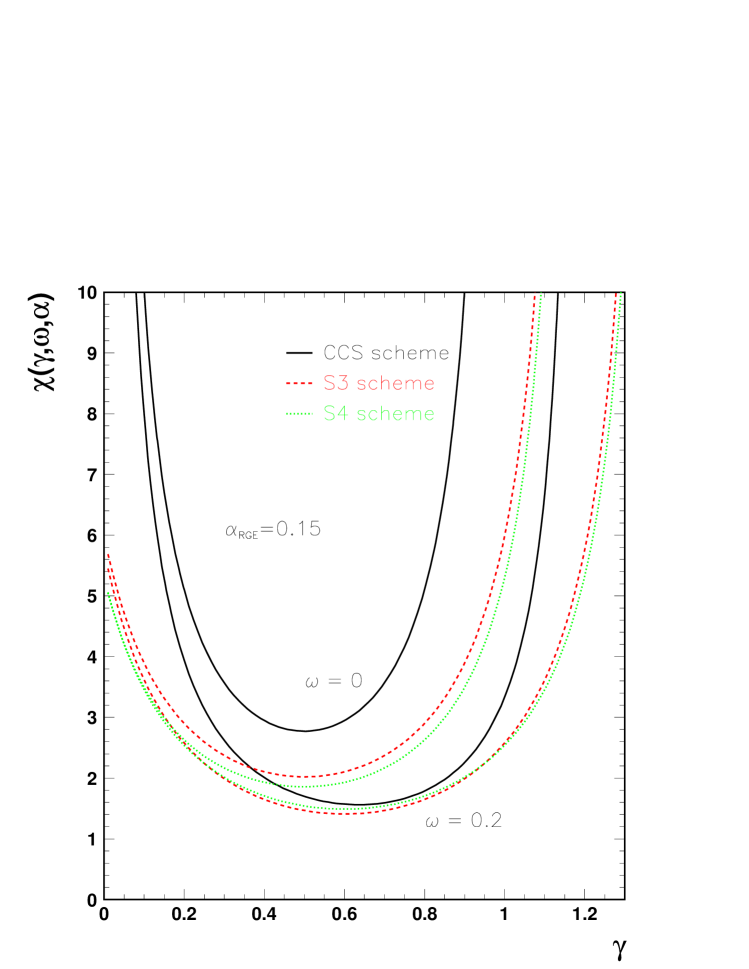
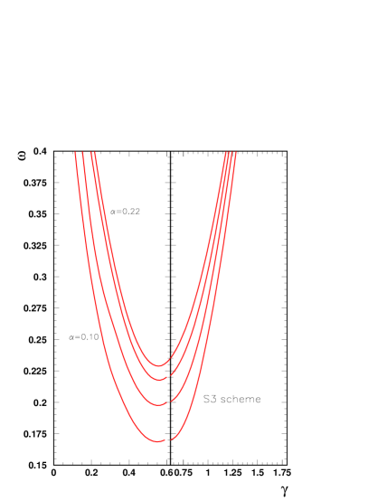
In Fig.1, we show for the three different schemes $\chi_{NLO}(\gamma,\omega)$ as a function of $\gamma$ for $\alpha_{RG}=0.15$ and for different values of $\omega$. In Fig.2, one finds the obtained kernels $\chi_{eff}(\gamma,\alpha_{RG})$ for the $CCS$ and $S3$ schemes, after solution of the implicit equation (5) for $\omega(\gamma,\alpha_{RG}).$

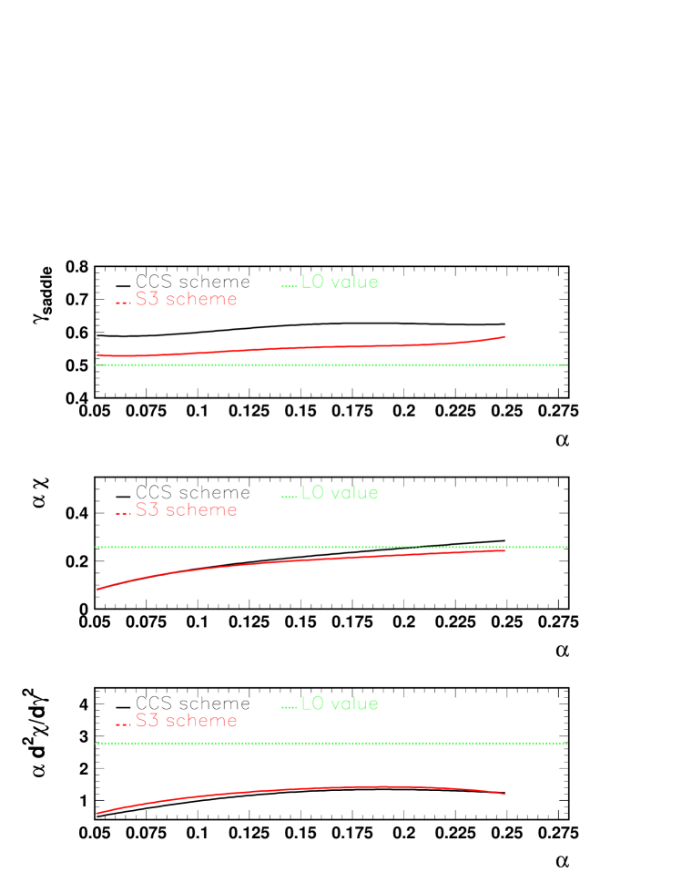
In Fig.3, one displays the parameter-independent values obtained for the set $\{\gamma_{c},\alpha_{RG}\ \chi_{eff}(\gamma_{c}),\alpha_{RG}\ \chi^{\prime\prime}_{eff}(\gamma_{c})\}$ as a function of $\alpha_{RG}.$ They result from a numerical analysis of the NLO effective vertices (for the $CCS$ and $S3$ schemes) in the vicinity of the saddle-point. Knowing the dependence $\alpha_{RG}(Q^{2}),$ they allow one to predict the behaviour of $F_{2},$ up to the determination of the free parameters $\cal N$ and $Q_{0},$ see (8). By comparison we show the corresponding values taken by the parameter-dependent set $\left\{\gamma_{c}\equiv{\scriptstyle\frac{1}{2}},\bar{\alpha}\chi_{LO}(\gamma_{c}),\bar{\alpha}\chi^{\prime\prime}_{LO}(\gamma_{c})\right\}$ which are the ingredients of the LO formula (4). It is interesting to note that the hard pomeron intercept $\alpha_{RG}\ \chi_{eff}(\gamma_{c})$ is compatible with the LO fitted value in a physical range of $\alpha_{RG}\sim.2$ while the LO value $\bar{\alpha}\sim.09$ is not physically motivated.

Let us come now to the quantitative analysis.

The parameters of the fits are given in Table I. Note that for the LO quantities $\bar{\alpha}$ is a fitted constant whereas in the NLO ones it is given by the standard renormalization group formula (6). However for completeness and inspired by theoretical arguments presented in Refs. thorne ; altar ; instabilities , we have also considered the LO expression (4), with the constant $\alpha_{s}$ replaced by the running coupling (6). The corresponding fit parameters are also given in Table I (referred as LO’(${\alpha}_{RG}$)).

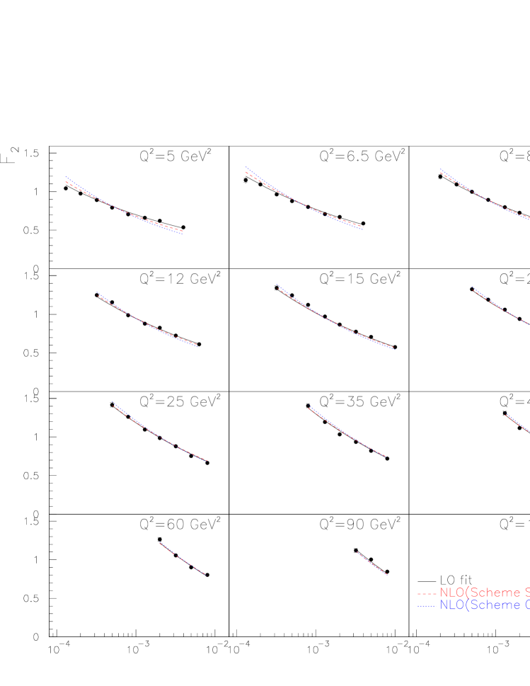
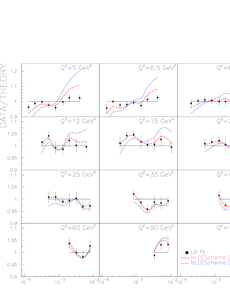
In Fig.4, we display the results of the BFKL fits to H1 data for LO and the $S3$ and $CCS$ schemes at NLO. As is clear from the figure the LO fit is doing a much better job than the considered NLO schemes (even considering that the NLO kernels depend on one less parameter). While the qualitative behaviour is correct they fail to take into account the quite precise $F_{2}$ data, especially at lower $Q^{2}$ where they show a too steep behaviour in $x_{Bj}.$ Note that the $S3$ scheme is somewhat better as confirmed by the value of the $\chi^{2},$ displayed in Table I. As obvious from Table I, the LO’(${\alpha}_{RG}$) fit (not represented in the figures) is not successful either.

In order to show the behaviour of the different fits with more detail, we display in Fig.5 the comparison of the ratio theory/data for the LO fit (with the expected error bars) and the NLO ones. This figure clearly confirms the problems at lower $Q^{2}.$

IV Analysis in Mellin space

In this section we want to analyze in more detail the features of the BFKL parametrizations and in particular the reasons of the still quantitatively unsatisfactory results of the NLO fits. For this sake, it is important to come back to the key ingredient of our analysis, i.e. the dominance of the hard Pomeron singularity expressed by the relation (5). As mentionned in section II, this relation is expressed in Mellin space, and our aim is now to make a phenomenological test of this relation directly in the $\omega$ space, without using the approximation of effective kernels.

Equality (5) can be checked at NLO using the GRV98 GRV98 , MRS2001 MRS2001 , CTEQ6.1 CTEQ6.1 and ALLM ALLM parametrisations. These four parametrisations give a fair description of the proton structure functions measured by the H1 and ZEUS collaborations over a wide range of $x_{Bj}$ and $Q^{2}$, as well as fixed target experiment data. The three first parametrisations correspond to a DGLAP NLO evolution whereas the ALLM one corresponds to a Regge analysis of proton structure function data. Since these parametrisations give a good description of data, we can use them to test easily the properties of the NLO BFKL consistency condition (5). This allows us to make a direct computation of the Mellin transform $\tilde{F}_{2}(\omega,Q^{2})$ of the proton structure function and study the NLO BFKL properties in Mellin space. Writing the Mellin transform as (cf. formula (1))

$$\tilde{F}_{2}(\omega,Q^{2})\equiv\int\frac{d\gamma}{2i\pi}\ \left(\frac{Q^{2}}{Q_{0}^{2}}\right)^{\gamma}\ {{\cal F}_{2}}(\gamma,\omega)\ ,$$ (10)

it is easy to realize that

$$\gamma^{*}(\omega,Q^{2})=\frac{{d}\ln\tilde{F}_{2}(\omega,Q^{2})}{{d}\ln Q^{2}}\ ,$$ (11)

where $\gamma^{*}$ is the saddle-point for the structure function, or in other well-known terms its effective anomalous dimension . Note that under our assumption that the saddle-point of the gluon Green function is transmitted to the full amplitude (see previous section) $\gamma^{*}\approx\gamma_{c}$, and thus the relation (11) allows for a phenomenological approach of the consistency condition.

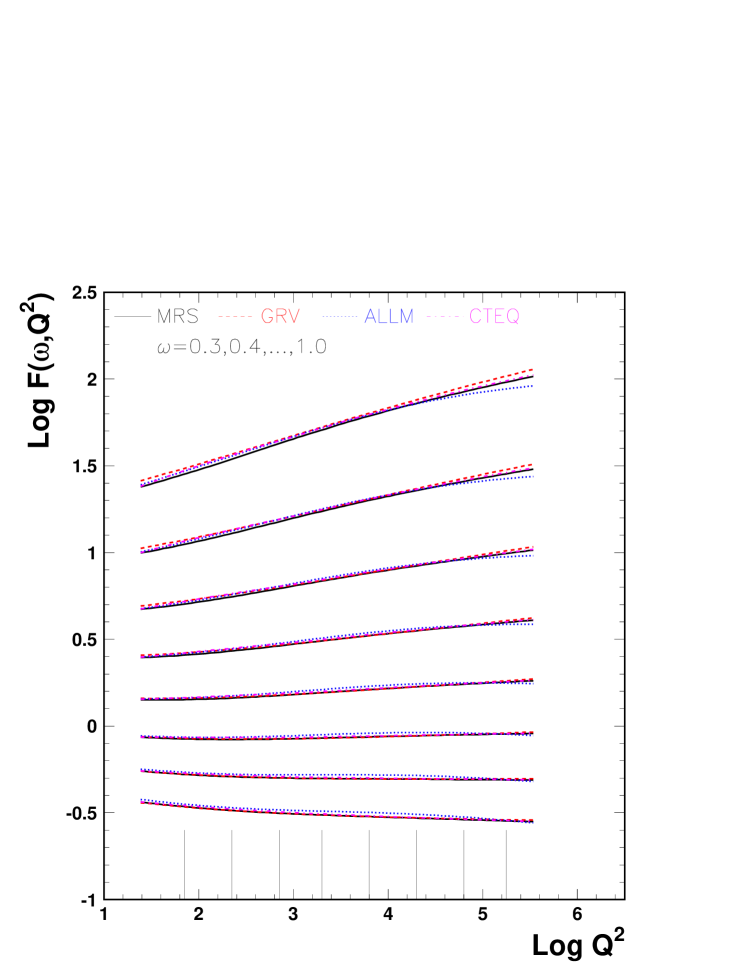
In Fig. 6, we display $\log\tilde{F}_{2}(\omega,Q^{2})$ as a function of $\log Q^{2}$ for the four parametrisations described above for different values of $\omega$. The upper curve corresponds to $\omega=0.3$, and $\omega$ varies in steps of 0.1 up to the down curve which corresponds to $\omega=1.0$. The limiting values in $\omega$ are due to the fact that, one the one hand, we do not want to use data at too high $x_{Bj}$ to test BFKL NLO properties and on the other hand, the data are lacking at very small $x_{Bj}$. We do not see large differences between the parametrisations used in this analysis. The slope in Fig. 6 gives directly the value of $\gamma^{*}$ according to formula (11). The vertical lines define the bins in $Q^{2}$ where the slope of $\tilde{F}_{2}(\omega,Q^{2})$ can be safely evaluated from the curves.

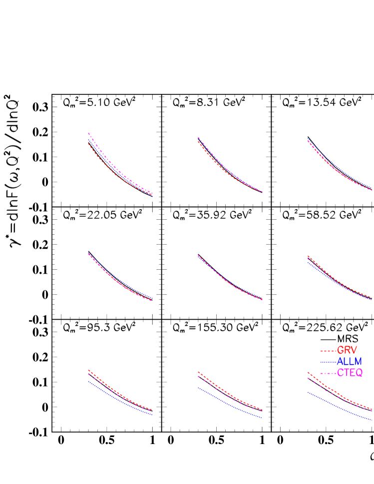
In Fig.7, we derive the values of $\gamma^{*}$ which are the slopes of $\log\tilde{F}_{2}$ in $\log Q^{2}$ in the different bins of $Q^{2}$ defined above, for the four parametrisations. We do not see sizable differences between the parametrisations except at higher values of $Q^{2},$ which are anyway not used in our analysis. Hence, in the kinematical range appropriate for BFKL phenomenology, the different sets of structure functions, being or not driven by the DGLAP equations, do not give rise to noticeable differences.

After having determined the values of $\gamma^{*}$, it is possible to test whether the NLO BFKL formula (5) admits a phenomenological verification, i.e. whether $\gamma_{c}\approx\gamma^{*}.$ In other words we have to check the consistency condition expressed as

$$\chi_{eff}(\gamma^{*}(\omega,Q^{2}),\alpha_{RG}(Q^{2}))=\frac{\omega}{\alpha_{RG}(Q^{2})}\ .$$ (12)

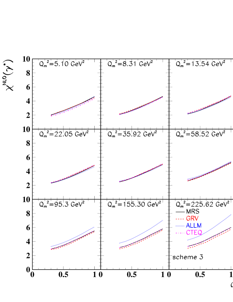
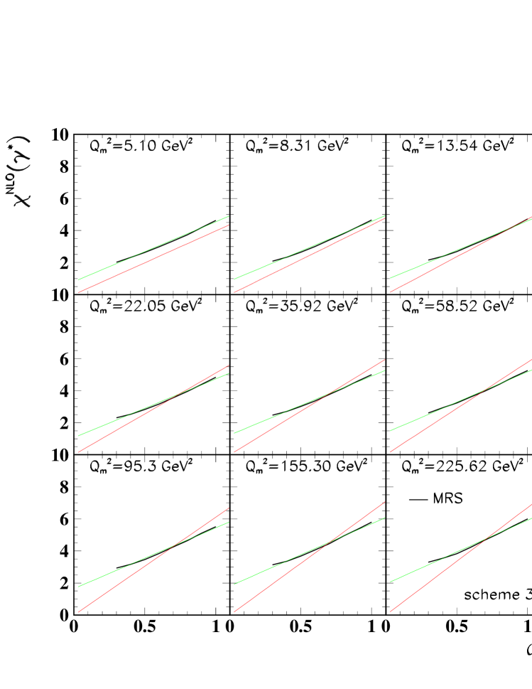
We considered (12) following the two resummation schemes defined in section II. For scheme $S3$ $\chi^{eff}$ as a function of $\omega$ is given in Fig.8. Note that the different parametrisations agree except at high values of $Q^{2},$ which are anyway out of the scope of our BFKL study.

Interestingly, while the scheme $S4$ (not shown in Fig.8) gives the same curves as for $S3,$ the same test could not be safely performed for the $CCS$ scheme. The reason is that a spurious pole appears in the quark sector at $\omega=1,$ when $\gamma^{*}\neq 0$ due to the incomplete momentum sum rule in the quark sector, which gives an effective anomalous dimension slightly below the value $0$ at $\omega=1$. This is a technical difficulty which requires a better treatment of the quark and gluon sectors simultaneously, which is still a challenge in the NLO BFKL approaches salambis .

We notice in Fig.8 that the linear property of relation (12), namely for $\chi_{eff}(\gamma^{*}(\omega,Q^{2}),\alpha_{RG}(Q^{2}))$ as a function of $\omega$ (12) is well verified. We indeed can describe the GRV and MRS parametrisations using a linear fit with a good precision. However the predicted zero at the origin $\omega=0$ is not obtained, even if the value at the origin remains small. The fit does not go through the origin and we would need to add a constant term to the linear fit formula. In order to quantify the observed discrepancy, we reformulated the phenomenologically obtained curves by the following formula:

$$\chi^{NLO}(\gamma^{*}(\omega,Q^{2}),{\alpha}_{in})={\omega}/{{\alpha}_{out}}\ ,$$ (13)

where ${\alpha}_{in}\equiv{\alpha}_{RG}$ is the theoretical input (6) while ${\alpha}_{out}$ is the phenomenologically determined slope of the linear fit displayed in Fig.9. The validity of (12) would obviously require ${\alpha}_{in}\equiv{\alpha}_{out}.$ In order to make the comparison, we have drawn the straight lines going from the origin, corresponding to the consistency condition (12).

We show in Fig.10, the values of $\alpha_{in}$ using the RGE equation (upper curve), and the values of $\alpha_{out}$ (lower curve), which are always smaller than the values of $\alpha_{RG}$. $\alpha_{out}$ is found to be closer to $\alpha_{in}$ at low $Q^{2}$ but more different from this value at higher values of $Q^{2}$.

BFKL fit	$\alpha$	$Q_{0}^{2}$	${\cal N}$	$\chi^{2}$ ( (/dof))
LO	0.092 $\pm$ 0.010	0.401 $\pm$ 0.012	.103 $\pm$ .002	1.33 (70)
LO’ (${\alpha}_{RG}$)	——	.055$\pm$ 0.23	1.055 $\pm$ .032	8.93 (71)
NLO (S3)	——	3.39 $\pm$ 0.23	.101 $\pm$ .003	3.13 (71)
NLO (CCS)	——	4.27 $\pm$ 0.30	.091 $\pm$ .007	8.62 (71)

Table 1: Results of the BFKL fits to the H1 data. LO BFKL ($\bar{\alpha}=cst.$): (1rst line); LO BFKL (${\alpha}_{RG}(Q^{2})$): (2nd line);NLO BFKL $S3$ scheme (3rd line); NLO BFKL $CCS$ scheme (4th line).

V Conclusion

Summarizing the results of our paper, we have confronted the predictions of BFKL kernels at the level of leading and next-leading logarithms (with resummation) with structure function data, using two different proposed types of resummation. Our method can be extended to other resummation proposals.

In a first stage we have proposed to use the “effective kernel” approximation of the NLO-BFKL kernels which, associated with the usual saddle-point approximation at high rapidity and large enough $Q^{2},$ allows one to obtain a simple two-parameter formula for the structure function $F_{2}.$ The comparison with the similar 3-parameter formula commonly used at LO level shows a deterioration of the fits when using two of the known resummed NLO schemes and a sensitivity to the different types of resummation.

In order to look for a more model-independent discussion of the discrepancy between precise data and the formulation in $x_{Bj}$-space, we perform an analysis of the kernel properties in Mellin-space. For this sake we find an interval in the energy-conjugate variable $\omega$ where the different Mellin transformed analyses from data give a definite answer within reasonable error bars. In Mellin-space, we find that small but sizeable effects give phenomenological deviations from the expected theoretical properties of the NLO kernels.

One possibility is that the saddle-point approximation we introduced is not valid. This simplicity assumption is phenomenologically motivated by its validity already at LO level. Unknown aspects of the prefactors, in particular the non-perturbative ones, could play a role in these deviations.

One way out is to look for higher order effects which could serve as a guide to improved resummation procedures of NLO BFKL kernels. hence, it deserves to investigate the phenomenological virtues of other proposed schemes and/or trying to make the suitable modifications to the known ones. Also, more precision in the discussion of NLO-BFKL predictions will soon be available with the completion of the perturbative NLO impact factors.

A possibility is to incorporate subasymptotic effects which go beyond the saddle-point approximation and may be computed from the NLO formulae altar ; instabilities ; salamalec . We expect our methods to be valid when incorporating these effects in the phenomenological analysis of $F_{2}$ data and thus further studies in the direction proposed in the present paper seem welcome.

Appendix

A.1 NLO-BFKL Schemes $S3$ and $S4$ of Ref.salam

Let us define the function

$$4\chi_{1}(\gamma)=-\left[\frac{2\beta_{0}}{C_{A}}\chi_{0}(\gamma)^{2}-K\chi_{0}(\gamma)-6\zeta(3)+\frac{\pi^{2}\cos(\pi\gamma)}{\sin^{2}(\pi\gamma)(1-2\gamma)}\left(3+\left(1+\frac{n_{f}}{C_{A}^{3}}\right)\frac{2+3\gamma(1-\gamma)}{(3-2\gamma)(1+2\gamma)}\right)-\right.$$

$$\left.-\psi^{\prime\prime}(\gamma)-\psi^{\prime\prime}(1-\gamma)-\frac{\pi^{3}}{\sin(\pi\gamma)}+4\phi(\gamma)\right]$$ (A.1)

where

$$\beta_{0}=\frac{11C_{A}}{12}-\frac{2n_{f}}{12}\ ;K=\frac{67}{9}-\frac{\pi^{2}}{3}-\frac{10n_{f}}{9C_{A}}$$ (A.2)

$C_{A}=3$ and $n_{f}=3,$

$$\phi(\gamma)\equiv\sum_{n=0}^{\infty}(-1)^{n}\left[\frac{\psi(n+1+\gamma)-\psi(1)}{(n+\gamma)^{2}}+\frac{\psi(n+2-\gamma)-\psi(1)}{(n+1-\gamma)^{2}}\right]$$ (A.3)

and

$$\chi_{0}(\gamma)=2\psi(1)-\psi(\gamma)-\psi(1-\gamma)\ .$$ (A.4)

We consider the asymptotic expansion of $\chi_{1}(\gamma)$ in $0:$

$$\chi_{1}(\gamma)=-\frac{1}{4}\left(\left(\frac{2\beta_{0}}{C_{A}}+3+\frac{2}{3}\left(1+\frac{n_{f}}{C_{A}^{3}}\right)\right)\frac{1}{\gamma^{2}}+\frac{2}{\gamma^{3}}+\left(-K+\frac{67+13\frac{n_{f}}{C_{A}^{3}}}{9}-\pi^{2}+4\psi^{\prime}(1)\right)\frac{1}{\gamma}-6\zeta(3)+\right.$$

$$\left.+\ \frac{395+71\frac{n_{f}}{C_{A}^{3}}}{27}-\frac{\pi^{2}}{2}-2\psi^{\prime\prime}(1)+2\psi^{\prime\prime}(1)\right)+O(\gamma)=-\frac{1}{2\gamma^{3}}-\left(\frac{\beta_{0}}{2C_{A}}+\frac{3}{4}+\frac{1}{6}\left(1+\frac{n_{f}}{C_{A}^{3}}\right)\right)\frac{1}{\gamma^{2}}+$$

$$+\left(\frac{K}{4}-\frac{67+13\frac{n_{f}}{C_{A}^{3}}}{36}+\frac{\pi^{2}}{4}-\psi^{\prime}(1)\right)\frac{1}{\gamma}\frac{3}{2}\zeta(3)-\frac{395+71\frac{n_{f}}{C_{A}^{3}}}{108}+\frac{\pi^{2}}{8}+O(\gamma)\ ,$$ (A.5)

and denote $d_{1,k}$ the coefficient of $\frac{1}{\gamma^{k}}$ in this expansion. In particular we get

$$d_{1,1}=-\frac{67}{36}-\frac{13n_{f}}{36C_{A}^{3}}+\frac{\pi^{2}}{12}+\frac{K}{4}\ ;d_{1,2}=-\frac{\beta_{0}}{2C_{A}}-\frac{11}{12}-\frac{n_{f}}{6C_{A}^{3}}\ ;d_{1,3}=-\frac{1}{2}\ .$$ (A.6)

We write

$$\chi^{(0)}(\gamma)=\chi^{(0)}(\gamma,\omega=\bar{\alpha}\chi^{(0)})=(1-\bar{\alpha}A)\ \left(2\psi(1)-\psi(\gamma+\frac{1}{2}\omega+\bar{\alpha}B)-\psi(1-\gamma+\frac{1}{2}\omega+\bar{\alpha}B)\right)$$ (A.7)

where $A,B$ are constants. The coefficient of the term in $\bar{\alpha}$ in the expansion of $\chi^{(0)}$ is

$$\chi_{1}^{(0)}(\gamma)=-\left(B+1/2\chi_{0}(\gamma)\right)(\psi^{\prime}(\gamma)+\psi^{\prime}(1-\gamma))-A\chi_{0}(\gamma)\ ,$$ (A.8)

whose asymptotic expansion in $0$ is given by

$$\chi_{1}^{(0)}=-(B+\frac{1}{2\gamma}+O(\gamma^{2}))(\frac{1}{\gamma^{2}}+2\psi^{\prime}(1-\gamma)+O(\gamma))-A(\frac{1}{\gamma}+O(\gamma^{2}))-\frac{1}{2\gamma^{3}}-\frac{B}{\gamma^{2}}-\frac{A+\frac{\pi^{2}}{6}}{\gamma}+O(1)\,.$$

Denoting $d^{(0)}_{1,k}$ the coefficient of $\frac{1}{\gamma^{k}}$ , one obtains

$$d^{(0)}_{1,1}=-A-\frac{\pi^{2}}{6}\ ;d^{(0)}_{1,2}=-B\ ;d^{(0)}_{1,3}=-\frac{1}{2}\ .$$ (A.9)

Hence,

$$\chi_{1}(\gamma)-\chi_{1}^{(0)}(\gamma)=(d_{1,2}-d_{1,2}^{(0)})\frac{1}{\gamma^{2}}+(d_{1,1}-d_{1,1}^{(0)})\frac{1}{\gamma}+O(1)\,.$$ (A.10)

Choosing A and B for eliminating spurious singularities in $0:$

$$A=-d_{1,1}-\frac{\pi^{2}}{6}\ ;B=-d_{1,2}\ .$$ (A.11)

we define

$$\chi^{(1)^{\prime}}(\gamma)=\chi^{(0)}(\gamma,\omega=\bar{\alpha}\chi^{(1)})=\chi^{(0)}(\gamma,\omega)+\bar{\alpha}(\chi_{1}(\gamma)-\chi_{1}^{(0)}(\gamma))\,.$$ (A.12)

The final NLO-BFKL kernel of $S3$ is finally given by performing the shift

$$\chi^{(1)}(\gamma)=\chi^{(1)^{\prime}}(\gamma-\frac{1}{2}\omega)\,.$$ (A.13)

For the scheme $S4$ of Ref.salam , instead of (A.7), one starts with

$$\chi^{(0)}(\gamma)=\chi^{(0)}(\gamma,\omega=\bar{\alpha}\chi^{(0)})=\chi_{0}(\gamma)-\frac{1}{\gamma}-\frac{1}{1-\gamma}+(1-\bar{\alpha}A)\left[\frac{1}{\gamma+\frac{1}{2}\omega+\bar{\alpha}B}+\frac{1}{1-\gamma+\frac{1}{2}\omega+\bar{\alpha}B}\right]\ .$$ (A.14)

One has

$$\chi_{1}^{(0)}(\gamma) = -A\left(\frac{1}{\gamma}+\frac{1}{1-\gamma}\right)-\left(\frac{1}{2}\chi_{0}(\gamma)+B\right)\left(\frac{1}{\gamma^{2}}+\frac{1}{(1-\gamma)^{2}}\right)=$$ (A.15)

$$= -A\left(\frac{1}{\gamma}+\frac{1}{1-\gamma}\right)-\left(\frac{1}{2\gamma}+B\right)\left(\frac{1}{\gamma^{2}}+\frac{1}{(1-\gamma)^{2}}\right)+O(1)$$

near 0. The singularity coefficients are now

$$d_{1,1}^{(0)}=-A-\frac{1}{2}\ ;\ d_{1,2}^{(0)}=-B\ ;\ d_{1,3}^{(0)}=-\frac{1}{2}\ .$$ (A.16)

Thus, to cancel the divergences of $\chi_{1}(\gamma)-\chi_{1}^{(0)}(\gamma)$, one is led to choose

$$A=-d_{1,1}-\frac{1}{2}\ ;\ B=-d_{1,2}\ .$$ (A.17)

$\chi^{(1)}(\gamma)$ is calculated as for $S3.$

A.2 NLO-BFKL Scheme $CCS$ autres as defined in trianta

Starting from the NLO-BFKL term $\chi_{1}(\gamma)$ as in [A.1], one first introduces the DGLAP splitting functions and their Mellin transforms, which are

$$P_{gg}(z)=\frac{z}{(1+z)_{+}}+\frac{1-z}{z}+z(1-z)+\frac{\beta_{0}}{2C_{A}}\,\delta(1-z)\ ;\ P_{qg}=\frac{N_{f}}{2N_{c}}[z^{2}+(1-z)^{2}]\ .$$ (A.18)

Giving

$$A_{gg}(\omega)=\int_{0}^{1}dz\,z^{\omega}P_{gg}(z)\;-\frac{1}{\omega}=\frac{\beta_{0}}{2C_{A}}-\frac{1}{1+\omega}+\frac{1}{2+\omega}-\frac{1}{3+\omega}-[\psi(2+\omega)-\psi(1)]\ ,$$ (A.19)

$$A_{qg}(\omega)=\int_{0}^{1}dz\,z^{\omega}P_{qg}(z)=\frac{N_{f}}{2N_{c}}\bigg{(}\frac{1}{1+\omega}-\frac{2}{2+\omega}+\frac{2}{3+\omega}\bigg{)}\ ,$$ (A.20)

one defines

$$A_{T}(\omega)=A_{gg}(\omega)+\frac{C_{F}}{N_{c}}A_{qg}(\omega),$$ (A.21)

with $C_{F}=(N_{c}^{2}-1)/2N_{c}$. One can write the pole structure of $\chi_{1}(\gamma)$ as

$$\chi_{1}(\gamma)=-\frac{1}{2\gamma^{3}}-\frac{1}{2(1-\gamma)^{3}}+\frac{A_{T}(0)}{\gamma^{2}}+\frac{A_{T}(0)-\frac{\beta_{0}}{2C_{A}}}{(1-\gamma)^{2}}-F\bigg{(}\frac{1}{\gamma}+\frac{1}{1-\gamma}\bigg{)}+{\rm finite},$$ (A.22)

where $F$, which vanishes when $N_{f}=0$ causing the simple poles to go away, is

$$F=\frac{N_{f}}{6N_{c}}\bigg{(}\frac{5}{3}+\frac{13}{6N_{c}^{2}}\bigg{)}\ .$$ (A.23)

Following the same extraction of spurious poles as previously, we are led to define

$$\tilde{\chi}_{1}(\gamma)=\chi_{1}(\gamma)-\frac{1}{2}\chi_{0}(\gamma)\chi^{\prime}_{0}(\gamma)+\frac{\chi_{0}(\gamma)}{(1-\gamma)^{2}}-\frac{1}{\gamma}+F\bigg{(}\frac{1}{\gamma}+\frac{1}{1-\gamma}\bigg{)}-\frac{A_{T}(0)}{\gamma^{2}}-\frac{A_{T}(0)-\frac{\beta_{0}}{2C_{A}}}{(1-\gamma)^{2}}\ ,$$ (A.24)

a function with no poles at all at $\gamma=0$ and $\gamma=1$. Next, one defines

$$\chi_{1}(\gamma,\omega)=\tilde{\chi}_{1}(\gamma)+\frac{1}{\gamma}-F\bigg{(}\frac{1}{\gamma}+\frac{1}{1-\gamma+\omega}\bigg{)}+\frac{A_{T}(\omega)}{\gamma^{2}}+\frac{A_{T}(\omega)-\frac{\beta_{0}}{2C_{A}}}{(1-\gamma+\omega)^{2}}\ .$$ (A.25)

Finally the full kernel is given by

$$\chi(\gamma,\omega)=\chi_{0}(\gamma,\omega)+\omega\,\frac{\chi_{1}(\gamma,\omega)}{\chi_{0}(\gamma,\omega)}\ ,$$ (A.26)

which has to be shifted as in (A.13).

Figure 1: $\chi_{NLO}$ as a function of $\gamma.$ The curves correspond to $\alpha=cte=0.15$ for two values of $\omega.$ Dark lines: $CCS$ scheme; dashed lines: $S3$ scheme; dotted lines: $S4$ scheme.

Figure 2: $\omega$ as a function of $\gamma$ for different values of $\alpha_{RG}.$ Left: $CCS$ scheme. Right: $S3$ scheme, see text. $\alpha_{RG}$ varies between 0.1 to 0.24 by steps of 0.02. For each value of $\omega$ in Eq.(5), two values of $\gamma$ are found and reported at each side of the minimum.

Figure 3: Determination of the saddle-point variables as functions of $\alpha_{RG}.$ Top: the saddle-point value $\gamma_{c};$ Middle: the effective Pomeron intercept $\alpha_{RG}\ \chi_{eff};$ Bottom: the effective diffusion variable $\alpha_{RG}\ \chi^{\prime\prime}_{eff}.$ The LO fixed values correspond to the fit of section III.

Figure 4: Results of the BFKL fits to the H1 data. LO BFKL kernel (continuous lines); NLO BFKL kernels ($S3$: Dashed lines, $CCS$: Dotted lines).

Figure 5: Ratio theory/data for the BFKL fits to the H1 data. LO BFKL: points with error bars; NLO BFKL Scheme $S3$: Dashed line; NLO BFKL Scheme $CCS$: Dotted line.

Figure 6: $\log F_{2}(\omega,Q^{2})$ as a function of $\log Q^{2}.$ Four different parametrisations of the proton structure function have been considered: MRS2001 (continuous), GRV98 (dashed), ALLM (dotted), CTEQ6.1 (dotted-dashed).

Figure 7: Derivation of the anomalous dimension $\gamma^{*}(\omega,Q^{2})$ by computing the slope of $logF_{2}$ as a function of $\log Q^{2}$.

Figure 8: Test of $\chi(\omega,Q^{2})$ for scheme $S3.$ The results for the four parametrizations are shown for the different bins in $Q^{2},$ (see text).

Figure 9: Phenomenological analysis of the effective kernel in Mellin space. Continuous lines:  $\chi_{eff}$. Dashed lines: linear approximation for as a function of $\omega.$ for the different bins of $Q^{2}$ and for scheme $S3.$ Continuous straight lines: consistency condution (12), see text

Figure 10: $\alpha$ as a function of $Q^{2}$: Obtained by RGE (upper curve) or as an output of the fit (lower curve) (see text).

References

- (1) G.Altarelli and G.Parisi, Nucl. Phys. B126 18C (1977) 298. V.N.Gribov and L.N.Lipatov, Sov. Journ. Nucl. Phys. (1972) 438 and 675. Yu.L.Dokshitzer, Sov. Phys. JETP. 46 (1977) 641.
- (2) L.N.Lipatov, Sov. J. Nucl. Phys. 23 (1976) 642; V.S.Fadin, E.A.Kuraev and L.N.Lipatov, Phys. lett. B60 (1975) 50; E.A.Kuraev, L.N.Lipatov and V.S.Fadin, Sov.Phys.JETP 44 (1976) 45, 45 (1977) 199; I.I.Balitsky and L.N.Lipatov, Sov.J.Nucl.Phys. 28 (1978) 822.
- (3) H1 Collab., C. Adloff et al, Eur.Phys.J. C21 (2001) 33; ZEUS Collab., S. Chekanov et al., Eur.Phys.J. C21 (2001) 443.
- (4) H Navelet, R.Peschanski, Ch. Royon, S.Wallon, Phys. Lett. B385 (1996) 357. S.Munier, R.Peschanski, Nucl.Phys. B524 (1998) 377.
- (5) A. Lengyel, M.V.T. Machado, Eur. Phys. J. A21 (2004) 145.
- (6) V.S. Fadin and L.N. Lipatov, Phys. Lett. B429 (1998) 127; M.Ciafaloni, Phys. Lett. B429 (1998) 363; M. Ciafaloni and G. Camici, Phys. Lett. B430 (1998) 349.
- (7) G.P. Salam, JHEP 9807 (1998) 019
-
(8)
M. Ciafaloni, D. Colferai, G.P.
Salam, Phys.Rev. D60 114036, , JHEP 9910 (1999) 017;
M. Ciafaloni, D. Colferai, G.P. Salam,A.M. Stasto, Phys.Lett. B541 (2002) 314. - (9) Stanley J. Brodsky, Victor S. Fadin, Victor T. Kim, Lev N. Lipatov, Grigorii B. Pivovarov, JETP Lett. 70 (1999) 155.
- (10) R.S. Thorne, Phys.Rev. D60 (1999) 054031 and references therein.
- (11) G. Altarelli, R.D. Ball, S. Forte, Nucl.Phys B621 (2002) 359, and references from the same authors therein.
- (12) J. J. Bartels, D. Colferai, S. Gieseke, A. Kyrieleis, Phys.Rev. D66 094017; For recent results: D. Y. Ivanov, M. I. Kotsky and A. Papa, The impact factor for the virtual photon to light vector meson transition hep-ph/0405297; J. Bartels, A. Kyrieleis, NLO Corrections to the Impact Factor: First Numerical Results for the Real Corrections to hep-ph/0407051.
- (13) M. Ciafaloni, D. Colferai, G. P. Salam and A. M. Stasto, Phys. Lett. B 541 314 (2002).
- (14) D.N. Triantafyllopoulos, Nucl.Phys. B648 (2003) 293. The formulation of the NLO kernel is provided in the appendix.
- (15) S. Munier, R. Peschanski, Nucl.Phys B524 (1998) 377.
- (16) M. Gluck, E. Reya, A. Vogt, Eur.Phys.J. C5 (1998) 461, for updated parametrizations.
- (17) A.D. Martin, R.G. Roberts, W.J. Stirling, R.S. Thorne, Eur.Phys.J. C23 (2002) 73.
- (18) D. Stump, J. Huston, J. Pumplin, W.-K. Tung, H.L. Lai, S. Kuhlmann, J. F. Owens, JHEP 0310 (2003) 046.
- (19) H. Abramowicz, E. Levin, A. Levy, U. Maor, Phys. Lett. B 269 (1991) 46.
- (20) G. P. Salam, private communication.
- (21) G. P. Salam, Asymptotics and preasymptotics at small x hep-ph/0501097.
- (22) J. Salomez, Le modèle des dipôles en QCD perturbative (in French), Saclay preprint T02/147 (2002), Diploma Mémoire for the “DEA Rhône-Alpin, ENS Lyon, France”. Available at: http://www-spht.cea.fr/articles/t02/147/.