Abstract

We use data on the deep inelastic structure function $F_{2}$ in order to constrain the cross-section for scattering a colour dipole off a proton. The data seem to prefer parameterisations which include saturation effects. That is they indicate that the strong rise with energy of the dipole cross-section, which holds for small dipoles, pertains only for $r<r_{s}(x)$ where $r_{s}(x)$ decreases monotonically as $x$ decreases. Subsequent predicitions for the diffractive structure function $F_{2}^{D(3)}$ also hint at saturation, although the data are not really sufficiently accurate.

1 Introduction

The possible observation of gluon saturation effects in the HERA data at very low $x$-values has been discussed extensively in the context of the colour dipole model. In particular, the “saturation model” of Golec-Biernat and Wüsthoff [1, 2] was shown some years ago to give an elegant and accurate account of deep inelastic scattering (DIS) at small $x$, and a rather good description of the diffractive deep inelastic scattering (DDIS) data [3, 4]. More recently, a new saturation model, the Colour Glass Condensate (CGC) model of Iancu, Itakura and Munier [5], has been formulated. This model, can be thought of as a more sophisticated version of the Golec-Biernat–Wüsthoff model. Gluon saturation effects are now incororated via an approximate solution of the Balitsky-Kovchegov equation [6], which applies in the perturbative region when the gluon densities become large and non-linear effects become important. The resulting dipole cross-section, obtained by fitting the free parameters of the model to the DIS data at low $x$, is very similar to that obtained in the original saturation model and Forshaw, Sandapen and Shaw [8] have shown that it leads to similar, successful, predictions for the DDIS data.

It is clear from this and other work [9] that the predictions of saturation models are compatible with a wide range of data. However, about the same time as the saturation model was formulated, Forshaw, Kerley and Shaw (FKS) proposed a two-component Regge dipole model [10] which explicitly excludes gluon saturation effects. As in the saturation model, the parameters of the model were tuned to fit the DIS data at low-$x$, and were subsequently shown [11] to give a good account of the DDIS data without further adjustment. Subsequently, the predictions of all three models for the DDIS data have been compared to each other [8], showing that they were all in good agreement with the data. However, at energies just above the measured region, the predictions of the saturation models and the unsaturated two component model rapidly diverge. A similar pattern emerges in deeply virtual Compton scattering [12] and vector meson production [7], although in the latter case, there are large ambiguities associated with the wavefunctions of the vector mesons.

From this it is clear that the data analysed to date are insufficient to establish the existence of gluon saturation. However, since the saturation model and the two-component Regge model were originally formulated, much more precise data have become available on both the DIS structure function $F_{2}$ [13] and the DDIS structure function $F_{2}^{D3}$ [14]. In this paper we will analyse these new data to see if they can throw more light on the question of gluon saturation.

2 Colour Dipoles and Saturation

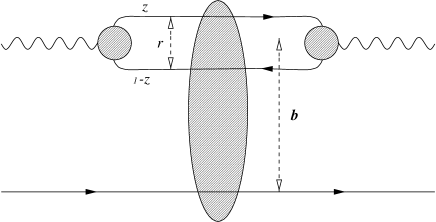
Figure 1: The colour dipole model for $\gamma^{*}p\to\gamma^{*}p$.

In the colour dipole model  [15, 16], the forward amplitude for virtual Compton scattering is assumed to be dominated by the mechanism illustrated in Figure 1 in which the photon fluctuates into a $q\bar{q}$ pair of fixed transverse separation $r$ and the quark carries a fraction $z$ of of the incoming photon light-cone energy. Using the optical theorem, this leads to

$$\sigma^{L,T}_{\gamma^{*}p}=\int dz\;d^{2}r\ |\psi_{L,T}(z,r)|^{2}\sigma(s^{*},r)$$ (1)

for the total virtual photon-proton cross-section, where $\psi_{L,T}(z,r)$ are the appropriate spin-averaged light-cone wavefunctions of the photon and $\sigma(s^{*},r)$ is the dipole cross-section. The dipole cross-section is usually assumed to be independent of $z$ (see below), and is parameterized in terms of an energy variable $s^{*}$ which depends on the model.

In the dipole model, not only the DIS total cross-section, but also the forward amplitudes for DDIS and DVCS, are determined by the same ingredients: the light-cone wavefunctions of the photon and the dipole cross-section. We shall briefly discuss each in turn.

For small $r$, the light-cone photon wavefunctions are given by the tree level QED expressions [15, 17]:

$$|\psi_{L}(z,r)|^{2} = \frac{6}{\pi^{2}}\alpha_{em}\sum_{f}e_{f}^{2}Q^{2}z^{2}(1-z)^{2}K_{0}^{2}(\epsilon r)$$ (2)

$$|\psi_{T}(z,r)|^{2} = \frac{3}{2\pi^{2}}\alpha_{em}\sum_{f}e_{f}^{2}\left\{[z^{2}+(1-z)^{2}]\epsilon^{2}K_{1}^{2}(\epsilon r)+m_{f}^{2}K_{0}^{2}(\epsilon r)\right\}$$ (3)

where $\epsilon^{2}=z(1-z)Q^{2}+m_{f}^{2}\;,$ $K_{0}$ and $K_{1}$ are modified Bessel functions and the sum is over quark flavours $f$ with quark masses $m_{f}$. These expressions decay exponentially at large $r$, with typical $r$-values of order $Q^{-1}$ at large $Q^{2}$ and of order $m_{f}^{-1}$ at $Q^{2}=0$. However for large dipoles $r\geq 1$fm, which are important at low $Q^{2}\leq 4m_{f}^{2}$, a perturbative treatment is not appropriate, and hadronic states of this transverse size are more sensibly modelled as pairs of constituent quarks, or vector mesons. For this reason, FKS [10, 11] used constituent quark masses, together with an enhancement factor in the region $r\approx 1$ fm, as suggested by Generalised Vector Dominance (GVD) ideas [18, 19, 20]. In contrast, the saturation models retain the perturbative wavefunction, but use a much smaller quark mass, which again enhances the wavefunction at large $r$. We have investigated both these approaches and find that the difference between them is only important when confronting the photoproduction data (mainly that from fixed-target experiments [21]). Since we are primarily interested in determining the need for saturation effects we will not need to consider these data here, and will therefore use the pertubative QED wavefunction (2) throughout, treating the quark mass as a parameter which can be used to adjust the wavefunction at large $r$-values. At high $Q^{2}$ where small dipoles dominate, the wavefunctions are insensitive to the quark mass.

Turning to the dipole cross-section, it is useful to distinguish three regions: small $r$, where pertubative ideas are relevant; large $r$, where typical “hadronic” behaviour is expected; and intermediate dipole sizes. The dipole formula (1) can be derived in the leading $\log(1/x)$ approximation of perturbative QCD [22]. In this approximation, the wavefunction is given by the perturbative expression (2) and the dipole cross-section is given by

$$\sigma(s^{*},r)=\frac{4\pi^{2}}{3}\alpha_{s}\int\frac{dk^{2}}{k^{4}}f(x,k^{2})(1-J_{0}(kr))\sim\frac{\pi^{2}r^{2}}{3}\alpha_{s}xg(x,A^{2}/r^{2}),$$ (4)

where $f(x,k^{2})$ is the unintegrated gluon density and the approximate equality holds for sufficiently small $r$ (with $A\sim 3$). As $x$ gets smaller, the gluon distribution grows rapidly, and the dipole cross-section in this region is sometimes approximated by the “hard pomeron” behaviour

$$\sigma(s^{*},r)\approx ar^{2}x^{-\lambda_{H}}$$ (5)

with $\lambda_{H}\approx 0.4$. At large $r\geq 1$ fm, which is important as $Q^{2}\to 0$, the models we discuss all build in “soft pomeron” behaviour

$$\sigma(s^{*},r)\approx\sigma_{0}s^{\lambda_{S}}\;,$$ (6)

with $\lambda_{S}$ small or zero. The dipole cross-section is then interpolated between the two in the intermediate $r$ region, in a way that depends on the specific model. For example, in the original Regge dipole model model of Forshaw, Kerley and Shaw [10, 11], the dipole cross-section was extracted from DIS and real photoabsorption data assuming a form with two terms, each with a Regge inspired $s$ dependence:

$$\sigma(s,r)=a_{soft}(r)s^{\lambda_{S}}+a_{hard}(r)s^{\lambda_{H}}\;$$ (7)

where the values $\lambda_{S}\approx 0.06$, $\lambda_{H}\approx 0.4$ resulting from the fit are characteristic of soft and hard diffraction respectively. The functions $a_{soft}(r)$, $a_{hard}(r)$ were chosen so that for small dipoles the hard term dominates yielding a behaviour $\sigma\rightarrow r^{2}(r^{2}s)^{\lambda_{H}}$ as $r\rightarrow 0$. This in accordance with the colour transparency ideas embodied in (4), since the dimensionless variable $r^{2}s$ is closely related to $x$ at large $Q^{2}$, where the typical dipole sizes $r\propto Q^{-1}$. For large dipoles $r\geq 1$ fm the soft term dominates with a hadronlike behaviour $\sigma\approx\sigma_{0}(r^{2}s)^{\lambda_{S}}$.

In any model which incorporates the “hard pomeron” behaviour (5), the dipole cross-section increases rapidly with decreasing $x$ for the small dipole sizes which dominate at large $Q^{2}$. In nature, however, one might expect this sharp rise to be softened by unitarity effects, an effect which we shall refer to as “gluon saturation” since, if it occurs in the region where (4) is valid, it can be interpreted as a dampening of the rapid increase of the gluon density with decreasing $x$ implied by (5). Such effects are not included in the FKS model [10, 11], where for a small dipoles of a given $r$, the behaviour (5) holds indefinitely as $x\rightarrow 0$. Non-linear saturation dynamics is, however, explicitly incorporated into the CGC model, in which the dipole cross-section is assumed to be of the form [5]

$$\sigma(x,r) = 2\pi R^{2}{\cal N}_{0}\left(\frac{rQ_{s}}{2}\right)^{2\left[\gamma_{s}+\frac{\ln(2/rQ_{s})}{\kappa\lambda\ln(1/x)}\right]}\hskip 28.45274pt\mathrm{for}\hskip 28.45274ptrQ_{s}\leq 2$$ (8)

$$= 2\pi R^{2}\{1-\exp[-a\ln^{2}(brQ_{s})]\}\hskip 28.45274pt\mathrm{for}\hskip 28.45274ptrQ_{s}>2~{},$$

where the saturation scale $Q_{s}\equiv(x_{0}/x)^{\lambda/2}$ GeV and $x=Q^{2}/(Q^{2}+s)$ is the Bjorken scaling variable. The parameters are fixed by a combination of theoretical constraints and a fit to DIS data. This dipole cross-section is characterised by a rapid increase with decreasing $x$, not dissimilar to (5), at small $r$, changing to a softer energy dependence as $r$ increases beyond

$$r_{s}(x)\equiv 2/Q_{s}=\;2(x/x_{0})^{\lambda/2}\;.$$

Saturation arises because of the decrease of the “saturation radius”, $r_{s}$, with decreasing $x$. Let us consider a dipole of fixed transverse size $r$. If $r<r_{s}(x)$, the dipole cross-section increases rapidly as $x$ decreases. However, this rapid rise eventually switches to a softer $x$ dependence when $x$ becomes so small that $r_{s}(x)$ itself decreases below the the fixed dipole size $r$.

Finally we remark that the word “saturation” is also often used to describe a somewhat different effect. In all models, the approximate $r^{2}$ dependence which pertains in the perturbative region at small $r$ is flattened when $r$ increases to values in the non-perturbative region. This “non-perturbative saturation” is important in describing the transition from high to low $Q^{2}$ values. However it is not what we are concerned with here.

3 Analysis of the HERA data

The parameters of the original Regge dipole model of FKS were determined using the DIS data available in 1999. However, since then more precise measurements of the deep inelastic scattering data in the diffractive region have been made at HERA [13], and there exists new data on DDIS [14]. In this section, we examine these newer data to see whether they can throw any new light on the issue of gluon saturation.

Our strategy is to confront the HERA data with a new Regge dipole model (which can be thought of as an update of the original FKS model to accommodate the latest data) and also a variant of that model which includes saturation. We shall also always compare to the predictions of the CGC saturation model.

Let us introduce our new and very simple Regge inspired dipole model. We shall assume that

$$\sigma(x_{m},r) = A_{H}r^{2}x_{m}^{-\lambda_{H}}~{}~{}{\mathrm{for}}~{}~{}r<r_{0}~{}~{}{\mathrm{and}}$$ (9)

$$= A_{S}x_{m}^{-\lambda_{S}}~{}~{}{\mathrm{for}}~{}~{}r>r_{1},$$

where

$$x_{m}=\frac{Q^{2}}{Q^{2}+W^{2}}\left(1+\frac{4m^{2}}{Q^{2}}\right).$$ (10)

For light quark dipoles, the quark mass $m$ is a parameter in the fit, whilst for charm quark dipoles the mass is fixed at 1.4 GeV.

In the intermediate region $r_{0}\leq r\leq r_{1}$ we interpolate linearly between the two forms of (9). Whether this is a Regge inspired model or a saturation model depends entirely upon the way in which the boundary parameter $r_{0}$ is determined.

3.1 Regge Fit to DIS data

If the boundary parameter $r_{0}$ is kept constant then the parameterisation reduces to a sum of two powers, as might be predicted in a two pomeron approach. It is plainly unsaturated, with the dipole cross-section obtained at small $r$-values growing rapidly with increasing $s$ at fixed $Q^{2}$ (or equivalently with decreasing $x$) without damping of any kind.

In all cases, we shall fit the electroproduction data in the kinematic range

$$0.045\,{\rm GeV}^{2}<Q^{2}<45\,{\rm GeV}^{2}\hskip 14.22636ptx\leq 0.01\;,$$ (11)

which is identical to that which was used to determine the parameters of the CGC saturation model.

The best fit obtained with what we shall henceforth call our FS2004 Regge fit is shown as the dashed line in Figure 2 (left) and the parameter values are listed in Table 1. While the values of the Regge exponents $\lambda_{S}$ and $\lambda_{H}$, and of the boundary parameters $r_{0}$ and $r_{1}$ are eminently sensible, the quality of the fit is not good, corresponding to a $\chi^{2}$/data point of 428/156. This is not just a failing of this particular parameterisation. We have attempted to fit the data with other Regge inspired models, including the original FKS parameterization, without success.

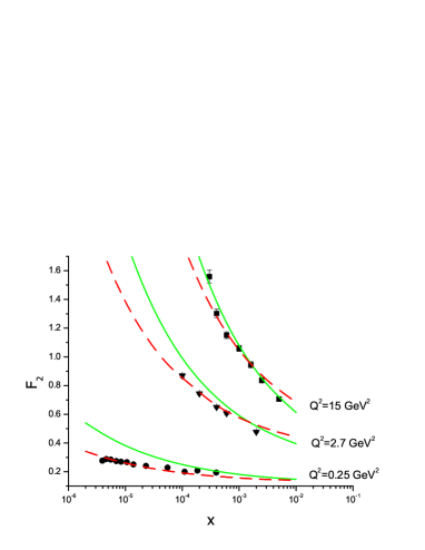
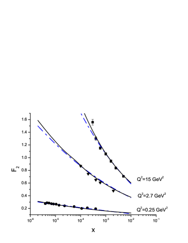
Figure 2: Comparison of our new dipole model fits to a subset of DIS data [13]. Left: No saturation fits. FS2004 Regge dipole fit (dashed line) and (solid line) a fit of the same model to data in the restricted range $5\times 10^{-4}<x<10^{-2}$, extrapolated over the whole $x$-range $x<0.01$. Right: Saturation fits. FS2004 saturation fit (solid line) and the CGC dipole model (dot-dashed line)

A possible reason for this failing is suggested by Figure 2 (left). At fixed-$Q^{2}$, the poor $\chi^{2}$ arises because the fit has much too flat an energy dependence at the larger $x$-values for all except the lowest $Q^{2}$ value. This could be corrected by increasing the proportion of the hard term, but this necessarily would lead to a steeper dependence at the lower $x$-values at all $Q^{2}$. This interpretation is confirmed by the solid curve in Figure 2 (left), which shows a the result of fitting only to data in the $x$-range $5\times 10^{-4}<x<10^{-2}$, and then extrapolating the fit to lower $x$-values, corresponding to higher energies at fixed-$Q^{2}$. As can be seen, this leads to a much steeper dependence at these lower $x$-values than is allowed by the data at all $Q^{2}$. An obvious way to solve this problem is by introducing saturation at high energies, to dampen this rise.

$$\begin{array}[]{c|c|c|c}\hline\cr A_{H}&0.650&\lambda_{H}&0.338\\ A_{S}&58.42&\lambda_{S}&0.0664\\ r_{0}&0.872&r_{1}&4.844\\ \hline\cr m&0.223&&\\ \hline\cr\end{array}$$ (12)

Table 1: Parameters for the FS2004 Regge model in the appropriate GeV based units.

We note that the aforementioned problem could also be resolved by restricting the fitted region to $x\leq 10^{-3}$. In our view, there is no justification for this, since the non-diffractive contributions are already small at $x\approx 0.01$. Furthemore, they make a positive contribution which decreases in size as $x$-decreases so that, to the extent that they are not completely negligible, they make the problem worse.

3.2 Saturation fits to DIS.

Saturation can be introduced into our new model by adopting a device previously utilized in [24]. Instead of taking $r_{0}$ to be fixed we now determine it to be the value at which the hard component is some fixed fraction of the soft component, i.e.

$$\sigma(x_{m},r_{0})/\sigma(x_{m},r_{1})=f$$ (13)

and treat $f$ instead of $r_{0}$ as a fitting parameter. This introduces no new parameters compared to our previous fit. However, the scale $r_{0}$ now moves to lower values as $x$ decreases, and the rapid growth of the dipole cross-section at a fixed value of $r$ begins to be damped as soon as $r_{0}$ becomes smaller than $r$. In this sense we model saturation, albeit crudely, with $r_{0}$ the saturation radius.

The best fit parameter values for what we refer to as our FS2004 saturation fit are listed in Table 2 corresponding to a $\chi^{2}$/data point of 155/156. The corresponding fits to the data are shown in Figure 2 (right). Also shown are the very similar results obtained using the more sophisticated CGC model (no charm fit) [5].

$$\begin{array}[]{c|c|c|c}\hline\cr A_{H}&0.836&\lambda_{H}&0.324\\ A_{S}&46.24&\lambda_{S}&0.0572\\ r_{1}&4.48&f&0.129\\ \hline\cr m&0.140&&\\ \hline\cr\end{array}$$ (14)

Table 2: Parameters for the FS2004 saturation model in the appropriate GeV based units.

It is clear from these results that the introduction of saturation into the model immediately removes the tension between the soft and hard components which is so disfavoured by the data. However, it is important to note that this conclusion relies on the inclusion of the data in the low $Q^{2}$ region: both the Regge and saturation models yield satisfactory fits if we restrict to $Q^{2}\geq 2\,{\rm GeV}^{2}$, with $\chi^{2}$/data point values of 78/86 and 68/86 respectively.

3.3 Predictions for DDIS

We finally seek support for our suggestion that saturation dynamics may already have been observed in the HERA data by turning to a comparison to data on diffractive deep inelastic scattering (DDIS).

In principle, if evidence for saturation is seen in DIS data, it should also be detectable at some level in DDIS data. As we have seen, there is a characteristic difference in the predictions of the Regge and saturation models for the energy dependence of the DIS structure function $F_{2}$ at fixed $Q^{2}$. If DIS and DDIS are described by the same dipole cross-section, then there should be corresponding differences in the predictions for the energy dependence of the diffractive structure function $F_{2}^{D(3)}$ at fixed $Q^{2}$ and fixed diffractively produced mass $M_{X}$. In the modern parlance, we shall examine the $x_{P}=(Q^{2}+M_{X}^{2})/(Q^{2}+s)$ distribution at fixed $\beta=Q^{2}/(M_{X}^{2}+Q^{2})$ and fixed $Q^{2}$.

A recent discussion of DDIS in the context of the dipole model, including the predictions of the CGC model, has been presented in reference [8] and we refer to that paper for the relevant formulae and more detailed discussion.

Our predictions involve no adjustment of the dipole cross-sections used to describe the $F_{2}$ data. However, we are free to adjust the forward slope for inclusive diffraction, $b$, within the range acceptable to experiment and in all cases we took $b=4.5$ GeV^-2. This simply influences the overall normalization of $F_{2}^{D(3)}$ which is therefore free to vary slightly. We are also somewhat free to vary the value of $\alpha_{s}$ used to define the normalization of the $q\bar{q}g$ component, which is important at low values of $\beta$. In all cases we choose $\alpha_{s}=0.1$.

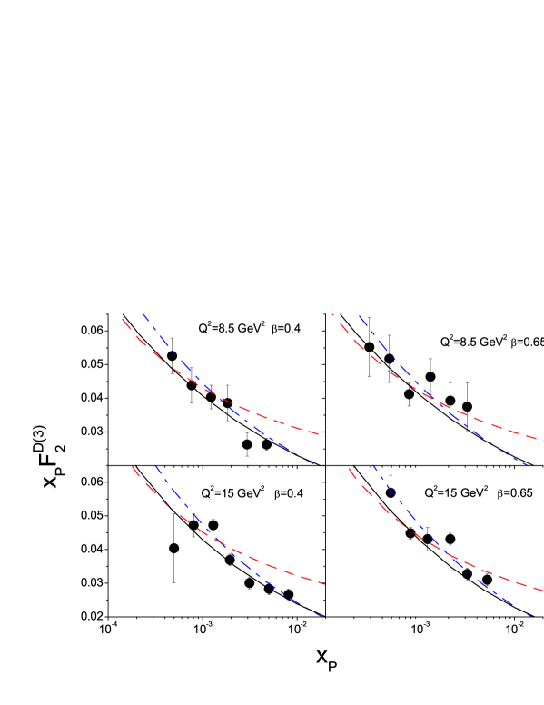
Figure 3: Comparison of the predictions of the FS2004 Regge fit (dashed line), the FS2004 saturation fit (solid line) and CGC fit (dot-dashed line) to the data on $F_{2}^{D(3)}$. Preliminary data from [14].

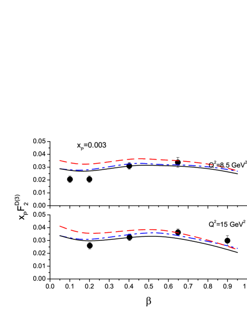
Figure 4: Comparison of the predictions of the FS2004 Regge fit (dashed line), the FS2004 saturation fit (solid line) and CGC fit (dot-dashed line) to the data on $F_{2}^{D(3)}$. Preliminary data from [14].

In Figure 3 we show the predictions of our new FS2004 Regge and saturation models for the $x_{P}$ dependence of the structure function $F_{2}^{D(3)}$ at fixed $Q^{2}$ and $\beta$, together with the corresponding predictions of the CGC model. In doing so, we have chosen to focus on $\beta$ values in the intermediate range where the predictions are relatively insensitive to the qq̄g term and to the large $r$ behaviour of the photon wavefunction, which are both rather uncertain.

There is, as expected, a characteristically different energy dependence of the Regge model and the two saturation models. There is a hint that the data prefer the saturation models, but more accuracy would be needed in order to make a more positive statement.

In Figure 4 we show the $\beta$ dependence at fixed $x_{P}$ and $Q^{2}$. Although this is unlikely to exhibit saturation effects in a transparent way, it is nonetheless a significant test of the dipole models discussed, because different size dipoles enter in markedly different relative weightings to the DIS case. For $\beta\geq 0.4$, where the $q\bar{q}$ dominates, it is clear that both the Regge dipole and both saturation models are compatible with the data, given the uncertainty in normalisation associated with the value of the slope parameter alluded to above. At the lowest $\beta$ values, where the model dependent $q\bar{q}g$ component is dominant, there is a discrepancy between the data and the predictions of all three models, which can only be removed by reducing the value of $\alpha_{s}$ well below the value assumed .

4 Conclusions

The colour dipole model offers a unified picture of diffractive photoprocesses over a wide range of $Q^{2}$. In this paper, we have attempted to throw light on the question of saturation in dipole models using both DIS and DDIS data.

To do this, we have used a particular dipole cross-section in which saturation effects can be included, or not included, in a simple way. When we speak of saturation we refer specifically to the effect whereby the rapid increase in energy of the contribution associated with small dipoles is damped at high enough energies. If there is no such damping, we say there is no saturation. Without saturation, we find that the model is unable to give a satisfactory account of the data, although the fit is better than with our original Regge dipole model [10] and many variations on it. Furthermore the discrepancies between data and fit are qualitatively of the sort which one might expect that saturation effects could remove. On incorporating such effects, we indeed obtain a very good fit to the data, without extra parameters, and the fit is of comparable quality to that obtained using the Colour Glass Condensate Model [5], which incorporates a more sophisticated treatment of saturation effects. Both models yield very similar, successful, predictions for the DDIS data in the regions where the $q\bar{q}$ dipole contribution dominates.

Finally, we note that the evidence we have presented for gluon saturation rests upon the applicability of the dipole model. It is of course well known that DGLAP fits to the DIS data work well down to $Q^{2}\sim 1$ GeV² [25, 26]. Such observations are in accord with our observation that the higher $Q^{2}$ data can be fitted without invoking saturation, and it is only on admitting the lower $Q^{2}$ data that the evidence emerges. However, Thorne has recently pointed out that DGLAP corrections to the dipole formulation are surely needed in order to make precise comparison to the data and therefore that any claims for saturation are to be viewed with caution [27]. This may well be a valid point and it will be interesting to see if our statement that saturation is responsible for alleviating the tension between the low and intermediate $Q^{2}$ data survives a more careful analysis.

5 Acknowledgement

This research was supported in part by a UK Particle Physics and Astronomy Research Council grant number PPA/G/0/2002/00471. We would like to thank Ruben Sandapen fruitful discussions. .

References

- [1] K. Golec-Biernat and M. Wüsthoff, Phys. Rev. D59 (1999) 014017.
- [2] K. Golec-Biernat and M. Wüsthoff, Phys. Rev. D60 (1999) 114023.
- [3] C. Adloff et al., H1 Collab., Zeit. Phys. C76 (1997) 613.
- [4] J. Breitweg et al., ZEUS Collab., Eur. Phys. J. C6 (1999) 43.
- [5] E. Iancu, K. Itakura and S. Munier, Phys. Lett. B590 (2004) 199.
- [6] I. Balitsky, Nucl. Phys. B463 (1996) 99; Yu.V. Kovchegov, Phys. Rev. D60 (1999) 034008.
- [7] J.R. Forshaw, R. Sandapen and G. Shaw, Phys.Rev. D69 (2004) 094013.
- [8] J.R. Forshaw, R. Sandapen and G. Shaw, Phys.Lett. B594 (2004) 283.
-
[9]
A.I. Shoshi, F.D. Steffen and H.J. Pirner, Nucl. Phys. A709 (2002) 131;
A. Kovner and U. Wiedemann, Phys. Rev. D66 (2002) 034031;
S. Munier, Phys. Rev. D66 (2002) 114012;
D. Kharzeev, E. Levin and L. McLerran, Phys. Lett. B561 (2003) 93;
E. Gotsman, E. Levin, M. Lublinsky and U. Maor, Eur. Phys. J. C27 (2003) 411;
L. Favart and M.V.T. Machado, Eur. Phys. J. C29 (2003) 365;
H. Kowalski and D. Tearney, Phys. Rev. D68 (2003) 114005;
J. Bartels, E. Gotsman, E. Levin, M. Lublinsky and U. Maor, Phys. Lett. B556 (2003) 114; ibid., Phys. Rev. D68 (2003) 054008;
E. Levin, hep-ph/0408039. - [10] J.R. Forshaw, G. Kerley and G. Shaw, Phys. Rev. D60 (1999) 074012.
- [11] J.R. Forshaw, G. Kerley and G. Shaw, Nucl. Phys. A675 (2000) 80.
- [12] M.F. McDermott, R. Sandapen and G. Shaw, Eur. Phys. J. C22 (2002) 665; J.R. Forshaw, R. Sandapen and G. Shaw, Proc. of the 26th Montreal-Rochester-Syracuse-Toronto (MRST) conference, 2004, hep-ph/0407261.
- [13] S. Chekanov et al., ZEUS Collab., Eur. Phys. J. C21 (2001) 442; C. Adloff et al., H1 Collab., Eur. Phys. J. C21 (2001) 33.
- [14] H1 Collaboration: Proc. of the International Europhysics Conference on High Energy Physics, Aachen, July 2003.
- [15] N.N. Nikolaev and B.G. Zakharov, Z. Phys. C49 (1991) 607; C53 (1992) 331.
- [16] A.H. Mueller, Nucl. Phys. B415 (1994) 273; A.H. Mueller and B. Patel, Nucl. Phys. B425 (1994) 471.
- [17] H.G. Dosch, T. Gousset, G. Kulzinger and H.J. Pirner, Phys. Rev. D55 (1997) 2602.
- [18] L. Frankfurt, V. Guzey and M. Strikman, Phys. Rev. D58 (1998) 094039.
- [19] H. Fraas, B. J. Read and D. Schildknecht, Nucl. Phys. B86 (1975) 346.
- [20] G. Shaw, Phys. Rev. D47 (1993) R3676; G. Shaw, Phys. Lett. B228 (1989) 125; P. Ditsas and G. Shaw, Nucl.Phys. B113 (1976) 246.
- [21] D.O. Caldwell et. al. Phys. Rev. Lett. 40 (1978) 1222.
- [22] L. Frankfurt, A. Radyushkin and M. Strikman, Phys. Rev. D55 (1997) 98.
- [23] A. Donnachie and P. V. Landshoff, Z. Phys. C61 (1994) 139
- [24] M. McDermott, L. Frankfurt, V. Guzey and M. Strikman, Eur. Phys. J. C16 (2000) 641.
- [25] A.D. Martin, R.G. Roberts, W.J. Stirling, R.S. Thorne, hep-ph/0410230
- [26] J. Pumplin, D.R. Stump, J. Huston, H.L. Lai, P. Nadolsky and W.K. Tung, JHEP 0207 (2002) 012.
- [27] R.S. Thorne, talk presented at DIS 2004, Prague (2004).