PSEUDO-AXIONS
IN LITTLE HIGGS MODELS

ABSTRACT

Little Higgs models have an enlarged global symmetry which makes the Higgs boson a pseudo-Goldstone boson. This symmetry typically contains spontaneously broken $U(1)$ subgroups which provide light electroweak-singlet pseudoscalars. Unless such particles are absorbed as the longitudinal component of $Z^{\prime}$ states, they appear as pseudoscalars in the physical spectrum at the electroweak scale. We outline their significant impact on Little Higgs phenomenology and analyze a few possible signatures at the LHC and other future colliders in detail. In particular, their presence significantly affects the physics of the new heavy quark states predicted in Little Higgs models, and inclusive production at LHC may yield impressive diphoton resonances.

1 Introduction

Little Higgs models [1] have recently emerged as an alternative solution to the naturalness problem of the Higgs sector in the Standard Model (SM). In these models, the origin of the electroweak (EW) scale is identified as new dynamics in the multi-TeV range that involves the spontaneous breaking of some extra continuous symmetry. While the exact nature of this dynamics, the UV completion, is undetermined — scenarios involving strong interactions [2], iterated Little Higgs models [3], or supersymmetry [4] have been proposed — the low-energy effective theory below the UV scale, $\Lambda$, is determined by the assumed symmetries. Various realizations of the Little Higgs symmetry structure have been proposed [5, 6, 7, 8, 9].

If at the scale $\Lambda$ an exact global (i.e., ungauged) symmetry is spontaneously broken, the spectrum contains Nambu-Goldstone bosons (NGBs) which are massless and have no renormalizable interactions. In analogy to low-energy QCD, we denote the would-be decay constant of these scalars by $F$. Naive dimensional analysis relates this scale to the cutoff $\Lambda$ by $F\sim\Lambda/4\pi$.

In Little Higgs models, the SM Higgs doublet is among these NGBs. This would be a natural explanation for a weakly interacting Higgs sector. However, since the Higgs doublet does have nontrivial renormalizable interactions — gauge, Yukawa, and self-couplings — there must be interactions in the initial Lagrangian which break the global symmetry explicitly. In general, such symmetry-breaking interactions introduce a one-loop Coleman-Weinberg potential [10] and a Higgs mass proportional to $m_{H}^{2}\sim\Lambda^{2}/(16\pi^{2})\sim F^{2}$. Without fine-tuning the parameters or adding additional fields, one then derives $F\sim v$, i.e., the new symmetry-breaking scale is near the electroweak symmetry breaking (EWSB) scale [11].

The new ingredient in Little Higgs models is the mechanism of collective symmetry breaking, as it was observed in the context of deconstructed extra-dimension models [12]. Each renormalizable scalar interaction breaks the postulated global symmetry explicitly, but leaves a continuous subgroup intact. Spontaneous breaking of this remaining global symmetry then still implies the existence of a massless NGB. However, all interactions together break all global symmetries explicitly, and no particle stays massless to all orders. The Higgs doublet is found among the scalars that still remain NGBs as long as only a single symmetry-breaking coefficient (spurion) is present in the Lagrangian, but acquire masses once all spurions are turned on. For instance, for two spurions $g_{1},g_{2}$ the resulting quadratic term in the effective Higgs potential is proportional to $(g_{1}/4\pi)^{2}(g_{2}/4\pi)^{2}\Lambda^{2}$. As usual, EWSB is triggered by such a term, and thus we have a three-scale model with

$$v\sim F/4\pi\sim\Lambda/(4\pi)^{2}\;.$$ (1)

Since the UV-completion scale $\Lambda$ is parameterically two orders of magnitude above the EW scale, any sign of the associated dynamics is strongly suppressed, and we are left with the virtual effects of new particles at the intermediate scale $F$. For a consistent implementation of collective symmetry breaking, enlarged symmetries must be introduced in all sectors of the model, so we expect new vector, spinor, and scalar particles with masses of order $F$. The low-energy traces of these particles can be computed and have been used to derive limits on the parameter space of any given Little Higgs model [13, 14, 15, 16, 17, 18, 19].

In this paper we study the phenomenological consequences of a particular property of the Little Higgs mechanism. To allow for an EW doublet among the NGBs, the spontaneous breaking of the global symmetry group typically involves a reduction of the group rank, e.g. $SU(3)\to SU(2)$. While the Higgs doublet in this example corresponds to the off-diagonal broken generators (analogous to the kaons in QCD), there is also one broken diagonal generator (analogous to the $\eta$). If there were no explicit symmetry-breaking terms, this particle, which acts as a pseudoscalar in its fermionic couplings, would behave as an axion, so we may call it the pseudo-axion of a Little Higgs model. Similar particles show up in other models which involve enlarged global symmetries, e.g. technicolor models [20, 21], see-saw topcolor models [22, 23], or the NMSSM [24, 25]. To determine the detailed model structure, one must experimentally establish any pseudo-axions as part of the Higgs sector and determine their properties. We find that these states have significant, broad impact on Little Higgs phenomenology.

2 Pseudo-axions in Little Higgs Models

In the bosonic sector, two different lines of model-building realize collective symmetry breaking. In models built along the lines of theory-space or moose models [1, 6, 7, 8, 9], the global-symmetry representation is reducible, i.e., in the scalar sector there are several distinct multiplets with gauge quantum numbers. The gauge coupling of any multiplet acts as a spurion which reduces the global symmetry down to the exactly realized gauge symmetry. This is spontaneously broken down to the EW gauge group $SU(2)\times U(1)$, and some NGBs are absorbed as the longitudinal components of new heavy vector bosons. However, if there are several scalar multiplets, there are not enough gauge bosons to absorb all the NGBs. The masses of the uneaten linear combinations are proportional to two or more spurions (i.e., gauge couplings) and do not appear up to one-loop order. Introducing scalar self-couplings as additional spurions, the structure becomes more complicated and more scalar multiplets are needed to keep the Little Higgs mechanism working, but the line of reasoning remains unchanged.

For concrete examples, let us consider the Minimal Moose [6] and Simple Group [7] models. In the first, with exactly one scalar coupling turned on, the global symmetry breaking is $[SU(3)]^{4}\to SU(3)$. The group rank is reduced by $k=6$ units, yielding $6$ pseudo-axion candidates. The rank of the spontaneously broken gauge group $SU(3)\times SU(2)\times U(1)$ is $r=2$ units larger than the SM EW group, so $2$ axions are eaten to make vectors massive and $k-r=4$ of them remain in the low-energy spectrum. (Two are EW singlets, while the other two are the neutral members of two real EW triplets.) Similarly, in the Simple Group model, if exactly one scalar coupling is turned on, the pattern of global symmetry breaking is $[SU(4)]^{3}\to[SU(3)]^{2}\times SU(2)$, while the gauge group is $SU(4)\times U(1)$. This yields $k=4$ and $r=2$, so there are $k-r=2$ pseudo-axions in this case.

As an alternative, some models implement an irreducible representation of the symmetry group in the scalar sector [5, 8]. In this case, to provide independent spurions in the gauge sector, the enlarged gauge symmetry must be such that part of it commutes with the EW gauge group. In this setting, for which the Littlest Higgs model [5] serves as an example, scalar self-couplings arise at one loop from integrating out the heavy vector bosons and fermions. Here, the global symmetry breaking is $SU(5)\to SO(5)$, with rank reduction $k=2$. If the extra gauge group is $SU(2)$, one pseudo-axion ($r=1$) is eaten in its symmetry breaking, and one ($k-r=1$) remains in the spectrum. On the other hand, if the extra gauge group is $SU(2)\times U(1)$, as originally proposed, both axions disappear from the spectrum.

This example demonstrates that the new particles become unphysical if all extra broken $U(1)$ symmetries are gauged. However, in that case we expect the corresponding number of new $Z^{\prime}$ bosons with masses of order $F$. These states are generally easy to detect at future colliders, either directly as resonances in $q\bar{q}$ or $e^{+}e^{-}$ annihilation [15, 26], or indirectly via the observation of contact interactions and of mixing with the standard $Z$ boson [13, 14]. In some models, these effects can be used to rule out much of the parameter space from existing data alone [13, 14, 15, 16, 17, 18, 19]. In the following, we therefore consider the situation where the extra groups are ungauged [15, 16, 17] and the pseudo-axions are physical.

3 Pseudo-axion Interactions

Let us consider the case of a single pseudo-axion which we denote by $\eta$. As an EW singlet it does not couple to EW gauge bosons at leading order. Furthermore, if $\eta$ is an exact NGB, it has no potential and does not couple to Higgs bosons either. However, in the fermion sector the situation is different. To account for Higgs Yukawa couplings, Little Higgs models contain interactions of fermions with the NGB multiplet, inducing Yukawa couplings for the axion. If the $U(1)$ symmetry generated by $\eta$ is parameterized by

$$\xi=\exp\frac{i}{F}\eta,$$ (2)

where $F$ is the symmetry breaking scale of the Little Higgs model, each field $\psi_{i}$ transforms like $\psi_{i}\to\xi^{\beta_{i}}\psi_{i}$, where $\beta_{i}$ is the corresponding $U(1)$ charge.

In some models, for some of the axions, these couplings are fixed by the symmetry structure that generates EWSB and can thus be deduced from the study of observables in the gauge, Higgs, or fermion sectors. In other models they cannot be determined this way. Typically, the axion interactions depend on additional parameters, so their observation provides independent information on the high-energy structure of the model. In the following, we present three specific models where axions play a role and discuss their interactions in some detail.

3.1 Mass and decays

For a phenomenological discussion of an $\eta$ axion, we need an estimate of its mass. If $\eta$ is an exact NGB, it would be exactly massless. This appears to be the case in some of the models we discuss in the following subsections. However, even then the $U(1)_{\eta}$ symmetry must be explicitly broken at some stage, so that $\eta$ picks up a mass; a massless particle coupled to fermions (even if this coupling is suppressed by $v/F$ and CKM factors) would induce a long-range force many orders of magnitude stronger than gravity and is therefore very strongly ruled out.

In general, the $U(1)_{\eta}$ symmetry will be anomalous. Then, if $m_{\eta}$ is below the QCD scale, $\eta$ becomes a Peccei-Quinn axion, which is ruled out for the parameter range of interest. Hence, we can assume a lower mass limit in the ${\rm GeV}$ range.

In any model, we can also put a rough upper limit on $m_{\eta}$ by considering its influence on the Higgs mass. To this end, we first note that a vertex $\eta^{2}H^{2}$ in the scalar potential would re-introduce a quadratic divergence in the Higgs mass at one loop, i.e., a correction $\Delta m_{H}^{2}\sim\Lambda^{2}/(16\pi^{2})\sim F^{2}$. If there is such a term, its coefficient should be parameterically of order $1/(16\pi^{2})$, so that the induced Higgs mass correction is at most of order $v^{2}$. Next consider $\eta H$ scattering: the NGB Lagrangian will contain derivative interactions of the form $\partial\eta^{2}\partial H^{2}/F^{2}$ which at one-loop order yield an effective $\eta^{2}H^{2}$ vertex with a quadratic divergence proportional to $(m_{\eta}^{2}/F^{4})\Lambda^{2}/(16\pi^{2})\sim m_{\eta}^{2}/F^{2}$. To keep this consistent without fine-tuning, we generally have to require $m_{\eta}\lesssim v$, i.e., the EW scale is an upper limit for the pseudo-axion mass.

All $\eta$ couplings to SM particles are suppressed by $v/F$, hence the rates for direct production are generically a factor of $(v/F)^{2}$ smaller than the corresponding Higgs production channels. For the decays, throughout the mass range we expect a similar pattern as for a light Higgs boson: dominant ($t\bar{t}$,) $b\bar{b}$, $\tau^{+}\tau^{-}$, … branching ratios (BRs), depending on kinematic accessibility, and some fraction of gauge-boson pairs, i.e., $gg$, $\gamma\gamma$, and $Z^{(*)}\gamma$, $ZZ^{(*)}$, $WW^{(*)}$. Since the axion is CP-odd, the vector-boson pair branching fractions are loop-induced and therefore stay small even above the thresholds for on-shell $WW$ and $ZZ$ pair production.

3.2 The Littlest Higgs model

Here we derive the pseudo-axion interactions in the Littlest Higgs model [5] with only one $U(1)$ gauged [15, 16, 17]. While this model has been extensively discussed in the literature, the pseudo-axion interactions have so far been ignored.

In this model, the NGB multiplet is parameterized by a $5\times 5$ matrix

$$\Xi=\left(\exp\frac{2i}{F}\Pi\right)\Xi_{0}\;,$$ (3)

where

$$\Xi_{0}=\begin{pmatrix}0&0&1_{2\times 2}\\ 0&1&0\\ 1_{2\times 2}&0&0\end{pmatrix}\quad{\rm and}\quad\Pi=\frac{1}{\sqrt{2}}\begin{pmatrix}\eta/\sqrt{10}&h&\phi\\ h^{\dagger}&-4\eta/\sqrt{10}&h^{T}\\ \phi^{\dagger}&h^{*}&\eta/\sqrt{10}\end{pmatrix}\;.$$ (4)

We have included only the physical states: the Higgs doublet, the $\eta$ singlet which multiplies the (canonically normalized) generator $\mathop{\rm diag}(1,1,-4,1,1)/2\sqrt{10}\,$, and $\phi$ which is a complex triplet written as a symmetric $2\times 2$ matrix. The triplet becomes heavy [i.e., its mass is of order $F$] and has little impact on low-energy phenomenology, so we ignore it in the following.

The kinetic term for the NGB multiplet is given by

$$\frac{F^{2}}{8}\mathop{\rm Tr}[(D_{\mu}\Xi)^{*}(D^{\mu}\Xi)]\,=\,|Dh|^{2}+\frac{1}{2}(\partial\eta)^{2}+\cdots\,,$$ (5)

which fixes the $\eta$ field normalization. In writing the Yukawa interaction we have to allow for $\eta$-dependent factors

$$\xi=\exp\frac{i}{\sqrt{5}\,F}\eta\;,$$ (6)

where the normalization has been adjusted for later convenience. The third-generation fermions are the left-handed quark doublet $q_{L}=(t_{L},b_{L})^{T}$, the right-handed singlet $t_{R}$, and the new singlets $T_{R},T_{L}$. We also define the matrices

$$\chi_{L}=\begin{pmatrix}i\tau^{2}\xi^{\beta_{0}}T_{L}&iq_{L}&0\\ -iq_{L}^{T}&0&0\\ 0&0&0\end{pmatrix}\quad{\rm and}\quad iT_{2}^{2}\,=\,\mathop{\rm diag}(0,0,-i\tau^{2\ast})/2\;.$$ (7)

With these definitions, the Yukawa interaction has the form [5, 19]

$$\mathcal{L}_{Y}^{t}=\lambda_{1}F\xi^{\beta_{1}}\bar{t}_{R}\mathop{\rm Tr}\left[\Xi^{*}(iT_{2}^{2})\Xi^{*}\chi_{L}\right]-\lambda_{2}F\xi^{\beta_{2}}\bar{T}_{R}T_{L}+\text{h.c.}$$ (8)

The parameters $\beta_{0,1,2}$ are real numbers determined by the differences of fermion $U(1)_{\eta}$ charges. The model has no prediction for these numbers (note that anomaly cancellation is not an issue since the $U(1)_{\eta}$ symmetry may well be anomalous), so we leave them as free parameters. In particular, we allow for $\beta_{2}\neq 0$. If this is the case, the $T$ quark mass is protected by a chiral symmetry and is therefore naturally of order $F$, the $U(1)_{\eta}$ breaking scale.

When the Yukawa interaction in Eq. (8) is expanded in powers of $1/F$, it yields a mass term for the new fermion $T$, a mixing of $t$ and $T$, a Higgs Yukawa interaction of the top quark, and higher-order terms:

$$\begin{split}\mathcal{L}_{Y}^{t}&=-\lambda_{1}F\bar{t}_{R}T_{L}-\lambda_{2}F\bar{T}_{R}T_{L}+\sqrt{2}\,\lambda_{1}\bar{t}_{R}h^{T}\tilde{q}_{L}\\ &\quad+\frac{i}{\sqrt{5}}(2-\beta_{0}-\beta_{1})\lambda_{1}\bar{t}_{R}\eta T_{L}-\frac{i}{\sqrt{5}}\beta_{2}\lambda_{2}\bar{T}_{R}\eta T_{L}+\cdots+\text{h.c.}\;,\end{split}$$ (9)

where $\tilde{q}_{L}=i\tau^{2}q_{L}$.

The mass matrix is diagonalized first by a rotation of the right-handed fields with the parameters

$$s=\lambda_{1}/\lambda\,,\qquad c=\lambda_{2}/\lambda\,,\qquad\lambda=\sqrt{\lambda_{1}^{2}+\lambda_{2}^{2}}\;,$$ (10)

which are expected to be ${\cal O}(1)$, and then by subsequent rotations of the left- and right-handed fields where the rotation angles are suppressed by powers of $v/F$. Keeping only the leading terms, we write the interactions in terms of the physical fields $H$ and $\eta$ and the quark masses $M_{T}=\lambda F$ and $m_{t}=sc\lambda v$, where $v$ is the Higgs vacuum expectation value:

$$\begin{split}\mathcal{L}_{Y}^{t}&=-\,M_{T}\,\bar{T}_{R}T_{L}\;-\,m_{t}\,\bar{t}_{R}t_{L}\\ &\quad+\,sc\frac{m_{t}}{F}\,H\bar{T}_{R}T_{L}\;-\,\frac{s}{c}\frac{m_{t}}{v}\,H\bar{T}_{R}t_{L}\;-\,\frac{m_{t}}{v}\,H\bar{t}_{R}t_{L}\\ &\quad+\,\frac{i}{cs}\frac{m_{t}}{v}\beta\,\eta\,\bar{T}_{R}T_{L}\;+\,i\frac{m_{t}}{v}\beta^{\prime}\,\eta\,\bar{t}_{R}T_{L}\;-\,i\frac{m_{t}}{F}\beta^{\prime\prime}\,\eta\,\bar{t}_{R}t_{L}\;+\,\cdots\,+\,\text{h.c.}\end{split}$$ (11)

The coefficients of the axion couplings depend on the fermion $U(1)_{\eta}$ charges as:

$$\beta =\;\frac{1}{\sqrt{5}}\left[(2-\beta_{0}-\beta_{1})s^{2}-\beta_{2}c^{2}\right],$$ (12a)

$$\beta^{\prime} =\;\frac{1}{\sqrt{5}}\left(2-\beta_{0}-\beta_{1}+\beta_{2}\right),$$ (12b)

$$\beta^{\prime\prime} =\;\frac{1}{\sqrt{5}}\left[(2-\beta_{0}+\beta_{2})s^{2}+\beta_{1}c^{2}\right]$$ (12c)

From the mass-eigenstate Lagrangian of Eq. (11) we can read off the vertex structure. By construction, $\eta$ is CP-odd. While the particular values of the Yukawa coupling coefficients are specific to a given model, their orders of magnitude with respect to the mass scales of the theory, shown in Table 1, are dictated by the $SU(2)$ transformation properties and thus are generic for Little Higgs models. The relation of the $T\bar{T}$ and $t\bar{t}$ couplings is a consequence of the fact that, after Little Higgs symmetry breaking, the heavy states are vectorlike, while $t$ is a chiral fermion. For $T\bar{T}$, unbroken EW symmetry forbids a coupling to the Higgs doublet, so this coupling must be proportional to $v/F$ which arises from $t-T$ mixing. Similarly, the coupling $t\bar{t}\eta$ is forbidden for unbroken symmetry since $\eta$ is a singlet. The chirality assignments of the mixed couplings are model-dependent: If the heavy singlet $T$ is replaced by a doublet, $P_{R}$ and $P_{L}$ have to be exchanged. For $T$ as a heavy triplet, the structure of $T\bar{t}H$ is unchanged while the $T\bar{t}\eta$ couplings are suppressed by $v/F$.

$$\begin{array}[]{|cc|}\hline\cr\bar{T}TH&{\cal O}(\frac{v}{F})\\ \bar{T}tH&{\cal O}(1)\,\mathcal{P}_{L}+{\cal O}(\frac{v}{F})\,\mathcal{P}_{R}\\ \bar{t}tH&{\cal O}(1)\\ \hline\cr\end{array}\qquad\begin{array}[]{|cc|}\hline\cr\bar{T}T\eta&{\cal O}(1)\,\gamma_{5}\\ \bar{T}t\eta&{\cal O}(1)\,\mathcal{P}_{R}+{\cal O}(\frac{v}{F})\,\mathcal{P}_{L}\\ \bar{t}t\eta&{\cal O}(\frac{v}{F})\,\gamma_{5}\\ \hline\cr\end{array}$$

Table 1: Chiral structure of the Yukawa couplings in Little Higgs models with a heavy $SU(2)$ singlet $T$. $P_{R,L}$ are the chirality projectors. For the coefficients, only the order of magnitude is indicated. This structure remains valid for the $\mu$ model presented in Sec. 3.3.

Although not previously defined in the literature, we posit that the Yukawa coupling for down-type fermions in the Littlest Higgs model can be written down as:

$$\mathcal{L}_{Y}^{b}=-\frac{\lambda_{b}}{\sqrt{2}}F\xi^{\beta_{3}}\overline{b}_{R}\mathop{\rm Tr}\left[\Sigma Y_{1}\chi_{L}\right]+\text{h.c.}\,,$$ (13)

where $Y_{1}$ is one of the hypercharge operators defined in [19],

$$Y_{1}=\frac{1}{10}\text{diag}(3,3,-2,-2,-2)\,.$$ (14)

The pseudoscalar coupling is then

$$g_{\eta bb}\overline{b}\gamma^{5}b\qquad\text{with}\qquad g_{\eta bb}=\frac{m_{b}}{\sqrt{5}F}\beta_{3}$$ (15)

Clearly, $\beta_{3}$ is an additional new free parameter.

The free parameters in the model are then one Yukawa coupling, $\lambda_{1}$, the mass scale $F$, and the four differences of $U(1)$ fermion charge assignments, $\beta_{0,1,2,3}$; $\lambda_{2}$ is fixed by the top quark mass condition. We consider the case $F=4$ TeV, which is motivated by the precision EW limits for the Littlest model [19].

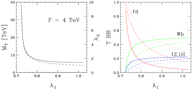
Figure 1: Left: $M_{T}$ (solid) v. $\lambda_{1}$ in the Littlest Higgs model with $F=4\,{\rm TeV}$. Also plotted is $\lambda_{2}$ (dashed), which is constrained by the choice of $\lambda_{1}$ and the known value $m_{t}$. Right: Heavy $T$ quark branching ratios to $Wb$ (green), $tZ/th$ (blue), and $t\eta$ (red), for three choices of the $U(1)_{\eta}$ charge differences $\beta_{0,1,2}$: 1,1,1 (solid); 1,0,1 (dashed); 0,0,1 (dotted).

The presence of the pseudo-axion $\eta$ alters the decay spectra of the heavy quark $T$ (see Appendix A), drastically for some regions of parameter space. Note in Eq. (11) that the $T\to t\eta$ partial width is proportional to $\beta^{\prime 2}$, which is a pure difference of the $\beta_{i}$ and contains no mixing factors, whereas the $T\to tH$ partial width is protected by $SU(2)$ and therefore appears only as a consequence of $T-t$ mixing. The latter is true also of the decays $T\to Wb,tZ\,$. (Ignoring mass effects, $\Gamma_{tH}=\Gamma_{tZ}=\frac{1}{2}\Gamma_{bW}\,$.) Due to the sum rule $1/\lambda^{2}_{t}=1/\lambda^{2}_{1}+1/\lambda^{2}_{2}$, both $\lambda_{1}$ and $\lambda_{2}$ must be larger than $\lambda_{t}$. While there is no general obstacle against $\lambda_{1}>\lambda_{2}$ (i.e. $\sin>\cos$), this is disfavored by large mixings of the third-generation EW currents [19]. So we take $\lambda_{1}$ to be bounded from below by $\lambda_{t}$, and from above by $\sqrt{2}\lambda_{t}$ using the condition $\lambda_{1}=\lambda_{2}$. This translates to a range $0.72<\lambda_{1}<1.02$. In Fig. 1 we plot $m_{T}$ v. the allowed values of $\lambda_{1}$, as well as the consequential $\lambda_{2}$, which closely tracks $m_{T}$. As expected, in the $\lambda_{1}\to\lambda^{SM}_{t}$ limit, $\lambda_{2}$ becomes large and almost totally responsible for $m_{T}$, which becomes (perhaps unnaturally, although one could argue that $\lambda_{1}=\lambda^{SM}_{t}$ is “natural” as well) much larger than $F$. For the lower extremal limit, $t-T$ mixing vanishes and the partial decay widths to $Wb,tZ,tH$ vanish correspondingly (the decoupling limit). The right-hand side of Fig. 1 shows the resulting $T$ BRs for three choices of the relevant $\beta_{i}$. For large mixing and equal $U(1)_{\eta}$ charges, BR($t\eta$) bottoms out at around $5\%$ and dominates only when the mixing becomes very small and $m_{T}$ grows quite large. For other choices of $\beta_{i}$, e.g. only $\beta_{2}\neq 0$, $\beta^{\prime}$ triples and BR($t\eta$) dominates everywhere, with the $T$ quark total width being ${\cal O}(10-100)$ GeV. For negative $\beta_{0,1}$, which are in no way unnatural, the non-$\eta$ decays would be practically squelched for all Yukawa couplings, and the total $T$ width can be hundreds of GeV. The shapes of all curves in Fig. 1 are independent of the choice of $F$.

The dominant decays of the $\eta$ are to $b\bar{b}$, $gg$ and $\gamma\gamma$, the latter two being loop-induced couplings (see Appendix B), and for $m_{\eta}>2m_{t}$, decays to top quark pairs. While there will also be loop-induced decays to $ZZ$ and $W^{+}W^{-}$, the BRs to observable final states are small fractions of the already rare decay rates, so we do not consider these further. There are in principle also direct couplings to the lighter fermions, but proportional to the fermion mass squared. We ignore these, as the only straightforward, high-efficiency signal would be to muons and that BR is typically an order of magnitude smaller than to photons. The BRs are independent of the scale $F$, since it appears the same way in all partial widths; and to the percent level, independent of $\lambda_{1}$. Table 2 shows the BRs to the dominant final states for various values of $m_{\eta}$. Note that from $m_{H}$ stability arguments we don’t expect $m_{\eta}\gtrsim v$, but this is order-of-magnitude, so we show one case with $m_{\eta}>2m_{t}$ for illustration.

$m_{\eta}$ [GeV] ($\beta_{i}$)	150 (1,1,1,1)	150 (1,0,1,1)	150 (1,1,1,0)	250 (1,1,1,1)	400
$\eta\to t\bar{t}$	$0\%$	$0\%$	$0\%$	$0\%$	$99.3\%$
$\eta\to b\bar{b}$	$38\%$	$72\%$	$0\%$	$17\%$	$0.02\%$
$\eta\to gg$	$61\%$	$29\%$	$99.7\%$	$83\%$	$0.5\%$
$\eta\to\gamma\gamma$	$0.17\%$	$0.08\%$	$0.27\%$	$0.27\%$	$0.002\%$

Table 2: Dominant branching ratios of the $\eta$ in the Littlest Higgs model. The case $\beta_{i}=(0,0,1,1)$ is identical to (1,0,1,1). For the case $m_{\eta}=400$ GeV, the $\beta_{i}$ assignments are irrelevant, as decay to top quark pairs overwhelmingly dominates.

It should be obvious that the phenomenology of the Littlest Higgs model has an extreme dependence on the presence of the pseudo-axion and the pattern of $U(1)_{\eta}$ fermion charge assignments $\beta_{i}$, which are undefined. It would not be inaccurate to say that the model is fairly incompletely defined. The situation is even more complicated than presented above, since there should be some $U(1)_{\eta}$ charge assignment for every SM fermion, greatly increasing the number of free parameters, although one could reasonably argue based on flavor-changing neutral current (FCNC) constraints that the charge assignments are identical at least across generations. Even the presence of just the third-generation $\beta_{i}$ introduces enough new parameters to present a serious phenomenological challenge at future colliders. The positive aspect of this is that measuring these parameters may provide clues to the model’s UV completion. Furthermore, the Little Higgs mechanism doesn’t depend on any of the $\beta_{i}$.

3.3 The $\mu$ model

Recently, Schmaltz has proposed a moose-type model [9] where the Little Higgs mechanism is implemented in a very economic way. A $\mu$ term which explictly breaks some of the global symmetry is responsible both for the absence of fine-tuning and for EWSB. The EW group is enlarged to gauged $SU(3)\times U(1)$. There are two nonlinear sigma model fields, each of which parameterizes a coset space $U(3)/U(2)$:

$$\Phi_{1}=\exp\biggl{[}i\frac{F_{2}}{F_{1}}\Theta\biggr{]}\begin{pmatrix}0\\ 0\\ F_{1}\end{pmatrix}\,,\qquad\Phi_{2}=\exp\biggl{[}-i\frac{F_{1}}{F_{2}}\Theta\biggr{]}\begin{pmatrix}0\\ 0\\ F_{2}\end{pmatrix}\,,$$ (16)

where 

$$\Theta=\frac{1}{F}\left\{\frac{\eta}{\sqrt{2}}+\begin{pmatrix}\begin{array}[]{cc}0&0\\ 0&0\end{array}&h^{*}\\ h^{T}&0\end{pmatrix}\right\}\,,\qquad F^{2}=F_{1}^{2}+F_{2}^{2}\;.$$ (17)

As usual, the global Little Higgs symmetry is broken radiatively by the gauge and Yukawa interactions that trigger EWSB and give the Higgs a mass, but they leave a global $U(1)_{\eta}$ symmetry intact. The Coleman-Weinberg mechanism thus generates a negative Higgs mass-squared and a positive quartic coupling, but without $U(1)_{\eta}$ breaking it does not contribute $\eta^{2}$, $\eta^{4}$, or $\eta^{2}h^{2}$ terms. These are generated only by the $\mu$ term:

$$-V=\;\mu^{2}\Phi_{1}^{\dagger}\Phi_{2}+\text{h.c.}=2F_{1}F_{2}\mu^{2}\cos\left(\frac{F\eta}{\sqrt{2}F_{1}F_{2}}\right)\Biggl{[}1-\frac{F^{2}}{2F_{1}^{2}F_{2}^{2}}(h^{\dagger}h)+\frac{F^{4}}{24F_{1}^{3}F_{2}^{3}}(h^{\dagger}h)^{2}+\ldots\Biggr{]}\,.$$ (18)

Thus, the complete potential up to quartic order is ($\kappa\equiv F_{1}/F_{2}+F_{2}/F_{1}\geq 2$):

$$-V=\;-(\delta m^{2}+\mu^{2}\kappa)(h^{\dagger}h)-\mu^{2}\kappa\frac{\eta^{2}}{2}+\left(\frac{\mu^{2}\kappa^{2}}{12F_{1}F_{2}}-\delta\lambda\right)(h^{\dagger}h)^{2}+\frac{\mu^{2}\kappa^{2}}{12F_{1}F_{2}}\left(\frac{\eta^{4}}{4}+\frac{3(h^{\dagger}h)\eta^{2}}{2}\right)+\ldots$$ (19)

Here, $\delta m$ and $\delta\lambda$ are the one-loop contributions to the Higgs boson mass and quartic coupling from the Coleman-Weinberg potential given in [9]. From this we read off the $\eta$ mass

$$m_{\eta}\;=\;\sqrt{\kappa}\,\mu\;\geq\;\sqrt{2}\,\mu.$$ (20)

To minimize the amount of fine-tuning, $\mu$ is chosen to be roughly of the order of the EW scale. Also from Eq. (19) we deduce the connection

$$m_{H}^{2}=-2(\delta m^{2}+m_{\eta}^{2})\;.$$ (21)

The interesting property of this model is that the $\eta$ mass is predicted, and can be calculated based on other experimental observables. In principle, only the masses of the Higgs boson and either the heavy $T$ quark or one heavy vector are needed to determine the scales $F_{1}$ and $F_{2}$. One can then calculate $\delta m^{2}$ [9] and predict $m_{\eta}$ by Eq. (21). However, $\delta m^{2}$ depends on the theory cutoff $\Lambda$ and has a noticeable dependence, so in practice performing precision fits to the model would be difficult, since the physical impact of the cutoff would not necessarily be clear. Nevertheless, within some reasonable uncertainty, measuring these values would be a first test of whether or not a discovery satisfied this particular model.

There are two possible gauge charge assignments for fermions in the $\mu$ model, called types I and II. The first has heavy partners of the top, charm and up quarks, and all generations carry identical gauge quantum numbers. This is, however, anomalous. This model also appears to be ruled out from precision EW data [9], so we do not discuss it further. The second model has slightly different charge assignments to eliminate the anomalies, and is not yet ruled out. In this scenario the top, strange and down quarks have heavy partners, and the Yukawa interactions are given by

$$\begin{split}\mathcal{L}&=-\,\lambda^{t}_{1}\overline{t}_{1,R}\Phi_{1}^{\dagger}\Psi_{T,L}\,-\,\lambda^{t}_{2}\overline{t}_{2,R}\Phi_{2}^{\dagger}\Psi_{T,L}\,-\,\frac{\lambda^{b}}{\Lambda}\epsilon^{ijk}\Phi^{i}_{1}\Phi^{j}_{2}\Psi^{k}_{T,L}\,\\ &\quad-\,\lambda^{d}_{1}\overline{q}^{d}_{1,R}\Phi_{1}^{\dagger}\Psi_{Q,L}\,-\,\lambda^{d}_{2}\overline{q}^{d}_{2,R}\Phi_{2}^{\dagger}\Psi_{Q,L}\,-\,\frac{\lambda^{u}}{\Lambda}\epsilon^{ijk}\Phi^{i}_{1}\Phi^{j}_{2}\Psi^{k}_{Q,L}\,\\ &\quad+\cdots+\text{h.c.}\end{split}$$ (22)

where the $SU(3)$ triplet is $\Psi_{T,L}=(\tau^{2}q^{3}_{L},T_{L})^{T}$ and $d,u$ sum over the first two generations; we assume the up-quark sector to be generationally diagonal, which is not necessary but simplifies the model. We diagonalize the mass matrix first with ${\cal O}(1)$ right-handed singlet-field rotations $t_{1,R}\to c\,t_{R}+s\,T_{R}$, $t_{2,R}\to-s\,t_{R}+c\,T_{R}$, with $s=\lambda_{1}F_{1}/M_{T}$ and $c=\lambda_{2}F_{2}/M_{T}$. We then rotate the left-handed fields by an ${\cal O}(v/F)$ angle $N_{1}m_{t}/M_{T}$ (see below). The leading (to ${\cal O}(v/F)$) Yukawa terms are

$$\begin{split}\mathcal{L}&=-M_{T}\,\overline{T}_{R}T_{L}-m_{t}\,\overline{t}_{R}t_{L}\\ &\quad-\frac{m_{t}}{v}\,H\overline{t}_{R}t_{L}-g_{\eta TT}\,H\overline{T}_{R}t_{L}+g_{\eta tt}\,H\overline{t}_{R}T_{L}+g_{HTT}\,H\overline{T}_{L}T_{R}\\ &\quad+ig_{\eta tt}\,\eta\,\overline{t}_{R}t_{L}+ig_{HTT}\,\eta\,\overline{T}_{R}t_{L}+i\frac{m_{t}}{v}\,\eta\,\overline{t}_{R}T_{L}+ig_{\eta TT}\,\eta\,\overline{T}_{R}T_{L}\\ &\quad+\cdots+\text{h.c.}\end{split}$$ (23)

where $m_{t}=\lambda_{1}\lambda_{2}vF/\sqrt{2}M_{T}$ and $M_{T}=\sqrt{\lambda_{1}^{2}F_{1}^{2}+\lambda_{2}^{2}F_{2}^{2}}\,$. The couplings are given by

$$g_{\eta tt}=\frac{m_{t}N_{2}}{\sqrt{2}F}-\frac{m_{t}^{2}N_{1}}{vM_{T}}\,,\qquad g_{\eta TT}=\frac{N_{1}m_{t}}{v}\,,\qquad g_{HTT}=-\frac{N_{1}^{2}m_{t}^{2}}{vM_{T}}+\frac{N_{3}v}{2M_{T}}\;,$$ (24)

with the abbreviations

$$N_{1}=\frac{F_{1}F_{2}}{F^{2}}\frac{\lambda_{1}^{2}-\lambda^{2}_{2}}{\lambda_{1}\lambda_{2}}\,,\qquad N_{2}=\frac{F_{2}^{2}-F_{1}^{2}}{F_{1}F_{2}}\,,\qquad N_{3}=\frac{\lambda_{1}^{2}F_{2}^{2}+\lambda_{2}^{2}F_{1}^{2}}{F^{2}}\;.$$ (25)

Comparing this with the Littlest Higgs model, we observe that here the axion properties are fully defined, i.e., no additional parameters have to be introduced. Furthermore, there are heavy partners of at least one quark and lepton of each generation. By contrast, in the Littlest Higgs model the presence of heavy fermions beyond the top-quark partner $T$ is not necessary.

We adopt the parameter set of Ref. [9], consistent with existing EW and flavor data and the preference for a light Higgs boson. The complete set of inputs, excluding the lepton sector, is $F_{1,2}$, $\lambda^{i}_{1,2}$, $\lambda^{b}$, $\lambda^{u}$, $\lambda^{d}$, and $\mu$. To simplify the set we assume $\lambda^{1,2}_{1}\ll\lambda^{1,2}_{2}\equiv\lambda^{t}_{2}$, so there is essentially no mixing between the SM down-type quarks and their heavy partners, whose masses are simply $\lambda_{2}F_{2}$. Deviations from this matter very little for the gross phenomenology. We further choose $\lambda^{t}_{1,2}$ to minimize $m_{T}$ given $F_{1,2}\,$ and $m_{t}$. $\lambda^{b}$ and $\lambda^{u}$ are fixed by $m_{b}$, $m_{c}$ and $m_{u}$. Our only free parameters are then $F_{1,2}$ and $\mu$, with the constraint that $F_{1}$ not be as small as the EW scale, $F\gtrsim 2$ TeV from EW precision constraints (primarily $\Delta T$ and four-fermion operators), and $F_{2}>F_{1}$ to avoid too much mixing which would lead to fermion non-universality. $F_{1}=F_{2}$ lies right at the edge of the limits on the latter. The cutoffs of the theory, $\Lambda_{1,2}$, are nominally $4\pi F_{1,2}$, but this is somewhat vague. Their precise choice affects the predicted Higgs mass, but because of the inherent uncertainty as to their definition we simply choose the suggested [9] value of $\Lambda_{1}=\Lambda_{2}\equiv\Lambda=5$ TeV and vary $\mu$ over a slightly broader range than the calculated $m_{H}$ would suggest is allowed or favored by data.

Starting then with the “Golden Point” in Ref. [9] of

$$F_{1}=0.5\,{\rm TeV},\quad F_{2}=2\,{\rm TeV},\quad\Lambda=5\,{\rm TeV}$$ (26)

we calculate

$$m_{T}=990\,{\rm GeV},\quad m_{S,D}=700\,{\rm GeV},\quad m_{Z^{\prime}}=1.2\,{\rm TeV},\quad m_{W^{\prime}}=950\,{\rm GeV}\,.$$ (27)

For $\mu\gtrsim 150$ GeV, $m_{H}$ is lower than the LEP direct exclusion limit of $\sim 114$ GeV. For $\mu\lesssim 120$ GeV we find that $m_{H}$ is greater than the SM $95\%\;{\rm c.l.}$ upper bound from precision EW data. However, in general in Little Higgs models, larger values of $m_{H}$ are allowed because of additional positive $\Delta T$ contributions from the other new content. We therefore do not restrict ourselves to a lower bound on $\mu$. For this Golden Point, as $\mu\to 0$, $m_{H}$ plateaus at around 450 GeV. To illustrate the dependence on $\Lambda$, if instead we explicitly set $\Lambda=4\pi F_{1}$ then only $\mu\gtrsim 135$ GeV is allowed. It is noteworthy that $m_{\eta}<2m_{t}$ for this parameter choice.

Figure 2: Left: $m_{\eta}$ v. $\mu$ for four choices of the ratio $F_{1}/F_{2}$: 1 (solid), 1/2 (dashed), 1/4 (dot-dashed), and 1/6 (dotted). Middle: $m_{H}$ v. $\mu$ for fixed $F_{2}=2.0$ TeV and various choices of $F_{1}/F_{2}$: 1 (solid), 1/2 (dashed) and 1/4 (dot-dashed). Right: $m_{H}$ v. $\mu$ for fixed $F_{1}/F_{2}=1/4$ and various $F_{1}$ [TeV]: 0.5 (solid), 1.0 (dashed), 1.5 (dot-dashed), and 2.0 (dotted).

Figure 3: $\eta$ branching ratios in the $\mu$ model for the Golden Point, as discussed in the text, as a function of $m_{\eta}$.

Moving away from the Golden Point, we observe several interesting features. First, while $m_{\eta}$ depends only on the ratio $F_{1}/F_{2}$ rather than their individual magnitudes, and grows larger for smaller ratios, for smaller ratios it is quite easy to violate the LEP direct exclusion limit on $m_{H}$. The trend for increasing ratio is shown in Fig. 2, left panel. The upper end of each curve is cut off by the condition that $m_{H}\gtrsim 114$ GeV. In general as $F_{1}/F_{2}$ approaches about 1/3, $m_{\eta}>2m_{t}$ becomes possible for $\mu\gtrsim 200$ GeV.

The right panel shows the (more complicated) trend for $m_{H}$. As $F_{1}$ moves closer to $F_{2}$, $m_{H}$ prefers to become quite heavy, although as both values become very large, this trend can reverse and $m_{H}$ becomes lighter. For example, $m_{H}$ plateaus at around 800 GeV for small $\mu$, although at the extremal point $F_{i}=3.3$ GeV the range of $m_{H}$ suddenly drops radically to around 100-200 GeV. For $F_{i}\gtrsim 3.4$ TeV, EWSB does not occur, providing a strong upper bound on the allowed values of $F_{i}$. For smaller ratios $F_{1}/F_{2}$, both the low-$\mu$ plateau for $m_{H}$ and the upper limit on $\mu$ become smaller. The latter is cut off by the Higgs becoming lighter than the LEP direct exclusion limit. A more thorough understanding of the allowed parameter space based on EW precision data would require a complete EW fit, which is beyond the scope of this work. We would still expect the EW data to prefer a light Higgs, but the upper limit could be considerably larger than in the SM, which is why we do not impose an upper limit on $m_{H}$ in Fig. 2.

Decays of the $\eta$ are more straightforward in this model than that of Sec 3.2, because all couplings are precisely defined. This is true for the $b\bar{b}\eta$ coupling as well, which in this model we derive to be

$$g_{\eta bb}\,=\,-\frac{N_{2}}{\sqrt{2}}\frac{m_{b}}{F}\;,$$ (28)

which is exactly like the $t\bar{t}\eta$ coupling (Eq. (23)), except that there is no term proportional to $N_{1}$ from mixing since there is no heavy partner of the $b$ quark. It has the interesting properties that it appears only at higher orders in the expansion of $\Phi_{1,2}$ (yet remains ${\cal O}(v/F)$), and that it is driven rapidly to zero as $F_{1}$ and $F_{2}$ approach each other. Couplings to muons and tau leptons will have the same form. The coupling to charm quarks will technically have the same form as that for top quarks, but here the mixing term is trivially small due to the ratio $m_{c}/M_{C}$. We can then straightforwardly predict the partial widths for $\eta$ to decay into SM particles.

However, there is one complication: unlike in the Littlest model, here there is a $ZH\eta$ coupling which arises from the kinetic term for $\Phi_{1},\Phi_{2}$ (note that both Higgs triplets have the same $SU(3)_{w}\times U(1)_{x}$ quantum numbers).

$$\mathcal{L}=(D_{\mu}\Phi_{1})^{\dagger}D^{\mu}\Phi_{1}+(D_{\mu}\Phi_{2})^{\dagger}D^{\mu}\Phi_{2}$$ (29)

with the covariant derivative expressed by the physical fields:

$$D_{\mu}\Phi_{k}=\partial_{\mu}\Phi_{k}+i\begin{pmatrix}eA_{\mu}+g\frac{c_{w}}{2}(1-t_{w}^{2})Z_{\mu}&\frac{g}{\sqrt{2}}W_{\mu}^{-}&0\\ \frac{g}{\sqrt{2}}W_{\mu}^{+}&-\frac{g}{2c_{w}}Z_{\mu}&0\\ 0&0&0\end{pmatrix}\Phi_{k}+\ldots\qquad k=1,2\;.$$ (30)

The dots stand for the part of the covariant derivative containing the five remaining heavy gauge bosons, which we leave out here. Plugging in the expansion of the nonlinear sigma-model Higgs fields, we derive a $ZH\eta$ coupling

$$\mathcal{L}_{ZH\eta}=\frac{m_{Z}}{\sqrt{2}F}N_{2}Z_{\mu}(\eta\partial^{\mu}H-H\partial^{\mu}\eta)$$ (31)

with $N_{2}$ defined previously. Such a coupling is forbidden for unbroken EW symmetry ($\eta$ is a singlet) so it must be proportional to $v/F$, but this is partially compensated for by large $N_{2}$ for the Golden Point.

We plot the BRs for $\eta$ to decay into SM particles, including the $ZH$ final state, in Fig. 3, as a function of $m_{\eta}$ for the Golden Point. Decays to the final state $b\bar{b}$ dominate for $m_{\eta}\lesssim 200$ GeV. Above this $gg$ dominates until the $ZH$ threshold is crossed at around $m_{\eta}=290$ GeV. Note that BR($\gamma\gamma$) remains non-trivial over an extremely large range of $\mu$. We can make a rough comparison with how a typical two-Higgs doublet model pseudoscalar behaves at low values of $\tan\beta$. Here, the role of $\tan\beta$ is played by the ratio of $\Phi$ decay constants, $F_{1}/F_{2}$. Due to constraint from lepton universality, we must have $F_{1}<F_{2}$, or $\tan\beta<1$, which is the opposite of what is required in e.g. the MSSM.

Although we do not plot the decay BRs for the Higgs, it is worth pointing out that for much of the parameter space where the $\eta$ does not decay to $ZH$, instead the decay $H\to Z\eta$ is kinematically allowed and constitutes a very large partial width. We discuss the impact of this on general Higgs sector phenomenology further in Sec. 4.

3.4 The original Simple Group model

The Simple Group model introduced in Ref. [7] displays an axion phenomenology that is a synthesis of the two previously discussed models. The low-energy effective theory contains two Higgs doublets. The global symmetry structure exhibits breaking of the semisimple group $[SU(4)]^{4}\to[SU(3)]^{4}$, while one $SU(4)$ subgroup is gauged and broken down to the SM gauge group $SU(2)$. Neglecting heavy singlet scalars, the four fundamental scalar multiplets can be approximately written as

$$\Phi_{1} \approx\;e^{+{\rm i}H/F}e^{+{\rm i}E_{u}/F}(0,0,F,0)^{T}\,,$$ (32)

$$\Phi_{2} \approx\;e^{-{\rm i}H/F}e^{-{\rm i}E_{u}/F}(0,0,F,0)^{T}\,,$$ (33)

$$\Psi_{1} \approx\;e^{+{\rm i}H/F}e^{+{\rm i}E_{d}/F}(0,0,0,F)^{T}\,,$$ (34)

$$\Psi_{2} \approx\;e^{-{\rm i}H/F}e^{-{\rm i}E_{d}/F}(0,0,0,F)^{T}\,.$$ (35)

The matrices are

$$H=\frac{1}{\sqrt{2}}\begin{pmatrix}\begin{matrix}0&0\\ 0&0\end{matrix}&\begin{matrix}h_{u}&h_{d}\end{matrix}\\ \begin{matrix}h_{u}^{\dagger}\\ h_{d}^{\dagger}\end{matrix}&\begin{matrix}0&0\\ 0&0\end{matrix}\end{pmatrix}\,,\qquad E_{U}=\frac{\eta_{u}}{6}\text{diag}(1,1,-3,1)\,,\quad E_{D}=\frac{\eta_{d}}{6}\text{diag}(1,1,1,-3)\;.$$ (36)

We introduce the abbreviations

$$\xi_{u/d}=\exp[{\rm i}\eta_{u/d}/(6F)]$$ (37)

to obtain

$$(\Phi_{1})_{i} \approx\;\xi_{u}^{3} \left[F\delta_{i,3}+\frac{{\rm i}}{\sqrt{2}}h_{u,j}\delta_{ij}\right],$$ (38)

$$(\Phi_{2})_{i} \approx\;\xi_{u}^{-3} \left[F\delta_{i,3}-\frac{{\rm i}}{\sqrt{2}}h_{u,j}\delta_{ij}\right],$$ (39)

$$(\Psi_{1})_{i} \approx\;\xi_{d}^{3} \left[F\delta_{i,4}+\frac{{\rm i}}{\sqrt{2}}h_{d,j}\delta_{ij}\right],$$ (40)

$$(\Psi_{2})_{i} \approx\;\xi_{d}^{-3} \left[F\delta_{i,4}-\frac{{\rm i}}{\sqrt{2}}h_{d,j}\delta_{ij}\right].$$ (41)

Considering the potential necessary to break EW symmetry, we can construct four bilinears $\Phi_{1}^{\dagger}\Psi_{1}$, $\Phi_{2}^{\dagger}\Psi_{2}$, $\Phi_{1}^{\dagger}\Psi_{2}$, and $\Phi_{2}^{\dagger}\Psi_{1}$. In those with like indices the Higgs doublets cancel, so these terms approximately vanish. The potential for $\eta$ is generated by the remaining terms

$$V_{\eta} =\;2b_{12}\text{Re}\left[\Phi_{1}^{\dagger}\Psi_{2}\right]+2b_{21}\text{Re}\left[\Phi_{2}^{\dagger}\Psi_{1}\right]\,,$$ (42)

namely,

$$\Phi^{\dagger}_{1}\Psi_{2}\approx F^{2}(\xi_{u}\xi_{d})^{3}\left(\exp[-2{\rm i}H/F]\right)_{34}=-(\xi_{u}\xi_{d})^{3}(h_{u}^{\dagger}h_{d})_{34}\;,\qquad\Phi^{\dagger}_{2}\Psi_{1}\approx(\Phi^{\dagger}_{1}\Psi_{2})^{\dagger}\;.$$ (43)

The coefficients $b_{ij}$ are expected to be of order $F^{2}$. The expansion in powers of $1/F$ yields

$$V_{\eta}=2(b_{12}+b_{21})\biggl{[}\text{Re}\left[h_{u}^{\dagger}h_{d}\right]-\frac{\eta_{u}+\eta_{d}}{2F}\text{Im}\left[h_{u}^{\dagger}h_{d}\right]-\frac{(\eta_{u}+\eta_{d})^{2}}{8F^{2}}\text{Re}\left[h_{u}^{\dagger}h_{d}\right]\biggr{]}.$$ (44)

Note that the $\eta$ couplings prefactor cannot vanish if EW symmetry is to be broken. Introducing the standard Higgs-field components (cf. also [16]), we get (as usual in 2-Higgs-doublet models, the scalar Higgs bosons are denoted by $h$ and $H$, the pseudoscalar by $A$)

$$\text{Re}\left[h_{u}^{\dagger}h_{d}\right] =\;\frac{1}{2}\left[(v_{1}+Hc_{\alpha}-hs_{\alpha})(v_{2}+Hs_{\alpha}+hc_{\alpha})+c_{\beta}s_{\beta}(A^{2}+2H^{+}H^{-})\right]$$ (45)

$$\text{Im}\left[h_{u}^{\dagger}h_{d}\right] =\;\frac{A}{2}\left[v_{1}c_{\beta}-v_{2}s_{\beta}+Hc_{\alpha+\beta}-hs_{\alpha-\beta}\right]$$ (46)

We observe that a potential is generated only for the linear combination $\eta_{+}=(\eta_{u}+\eta_{d})/\sqrt{2}$. This pseudo-axion is analogous to the one in the $\mu$ model. However, the mass of $\eta_{+}$ is very low, of order $v^{2}/F$. A further effect of the above potential is mixing of $\eta_{+}$ with the pseudoscalar $A$ of the second Higgs doublet, suppressed by $v/F$.

The orthogonal combination $\eta_{-}=(\eta_{u}-\eta_{d})/\sqrt{2}$ remains massless, similar to the $\eta$ of the Littlest Higgs model. Without introducing extra symmetry-breaking terms we have no prediction for $m_{\eta_{-}}$.

Due to the mixing interaction, there is an $h\eta_{+}\eta_{+}$ vertex with a coupling of the order $v^{3}/F^{2}$. This modifies the standard Higgs width by an amount of

$$\Gamma_{H\to\eta_{+}\eta_{+}}\sim\frac{1}{16\pi}\sqrt{1-\frac{4m_{\eta_{+}}^{2}}{m_{H}^{2}}}\frac{v^{5}}{F^{4}}\sim\frac{15}{\left(F[\text{TeV}]\right)^{4}}\;{\rm MeV},$$ (47)

and gives a BR of order $5-10\%$ into an $\eta_{+}$ pair. This decay may be detectable when measuring Higgs BRs at a future linear collider.

The quark Yukawa Lagrangian with $\eta$’s present is

$$\mathcal{L}_{Y}= \;\lambda_{1}\overline{\chi}_{1,R}\chi_{1,L}F\xi_{u}^{3}+\lambda_{2}\overline{\chi}_{2,R}\chi_{1,L}F\xi_{u}^{3}+\lambda_{3}\overline{\chi}_{3,R}\chi_{1,L}F\xi_{d}^{3}$$

$$+\lambda_{1}\sqrt{2}{\rm i}(\overline{\chi}_{1,R}h_{u}^{\dagger}q_{L})\xi_{u}^{3}-\lambda_{2}\sqrt{2}{\rm i}(\overline{\chi}_{2,R}h_{u}^{\dagger}q_{L})\xi_{u}^{3}-\lambda_{2}\sqrt{2}{\rm i}(\overline{\chi}_{3,R}h_{d}^{\dagger}q_{L})\xi_{d}^{3}\;.$$ (48)

Ignoring the coupling $\lambda_{1}$ (light quark limit) as well as $\lambda_{d}$ (for the down-type quarks) [16], and inserting the vacuum expectation values of the Higgs fields and keeping at most trilinear terms, we obtain the fermion mass matrix

$$(\overline{\chi}_{1,R},\overline{\chi}_{2,R},\overline{\chi}_{3,R})\begin{pmatrix}0&0&0\\ \lambda_{2}v\cos\beta\cos\gamma\xi_{u}^{3}&\lambda_{2}F\xi_{u}^{3}&0\\ \lambda_{3}v\sin\beta\sin\phi\xi_{d}^{3}&0&\lambda_{3}F\xi_{d}^{3}\end{pmatrix}\begin{pmatrix}t_{L}\\ \chi_{1,L}\\ \chi_{2,L}\end{pmatrix}\,.$$ (49)

Here the additional angles $\gamma$ and $\phi$ parameterize different scales within different Higgs multiplets. One linear combination of $\overline{\chi}_{2,R}$ and $\overline{\chi}_{3,R}$ is the right-handed top quark, while the orthogonal linear combination mixes with $\chi_{1,L}$ and $\chi_{2,L}$ to give two heavy quarks with masses of the order $F$. Here, the physically relevant rotation is between the left-handed fermions. The resulting structure of the $\eta$ couplings is determined by the general rules given in Sec. 3.2. Regarding the couplings, the $\eta_{+}$ is something like a pseudoscalar Higgs rendered ultralight by a sort-of Little see-saw mechanism between the scales $v$ and $F$. In contrast, the $\eta_{-}$ is a pseudo-axion in the pure sense, with similar properties as described in the previous section.

The extreme complexity of this model is manifest. We therefore do not try to examine its phenomenology in detail. Rather, we wish to point out generically that the addition of more heavy quark and lepton partners can multiply the partial widths of the $\eta$ to $gg$ and $\gamma\gamma$, which would in general increase the $gg\to\eta\to\gamma\gamma$ rate at hadron colliders, discussed in the next section.

4 Phenomenology

We concluded in the previous section that the $\eta$ coupling structure to SM fermions and gauge bosons resembles the couplings of a CP-odd Higgs boson. Compared to standard two-Higgs doublet model interactions, however, there are three important differences: (i) all couplings to SM particles are suppressed by a common factor $v/F$, which reduces direct production rates by $(v/F)^{2}$, although for $gg\to\eta$ at hadron colliders this may be compensated by the presence of multiple heavy particles running in the loop; (ii) the $Tt\eta$ coupling is not suppressed and can be similar in magnitude to $Tth$, altering the phenomenology of the new heavy quarks from that expected by strict $SU(2)$ symmetry; (iii) the $ZH\eta$ interaction is not allowed in all models.

4.1 Production related to heavy $T$ quarks at hadron colliders

The pseudo-axion $\eta$ has essentially Yukawa couplings to the SM fermions, which are large for the top quark. Thus, one would anticipate that associated $t\bar{t}\eta$ production would occur, analogous to top-pion [27] or two-Higgs doublet model pseudoscalar production [28] but the $(v/F)^{2}$ suppression factor renders this channel useless by trivial comparison to the SM Higgs. While the rate for $T\bar{T}$ is not suppressed by $(v/F)^{2}$, it is unfortunately hugely phase-space suppressed: the $T\bar{T}$ rate is already sub-fb level.

However, the $T$ quark can decay to $t\eta$, often with significant BR and sometimes dominantly. At a minimum the $T$ quark phenomenology is changed in a non-trivial way, since the $\eta$ does not participate in $SU(2)$. Because the coupling is highly model-dependent, and not even completely defined in some models, predictions rapidly become exercises in having too many free parameters. On the other hand, precisely measuring all BRs, both to the “standard” final states $tH$, $tZ$, and $bW$ [17], and to $t\eta$, could provide deep insight into the full structure of the model that is realized in nature, if the Little Higgs mechanism is discovered.

Heavy $T$ quarks can be produced at hadron colliders singly or in pairs, analogous to SM $t$ quark production. However, in general the single-$T$ rate is larger than that for $T\bar{T}$ because of the enormous phase-space suppression in heavy pair production. Consequently, only single-$T$ phenomenology has been studied seriously [29]. This study found that even observing TeV scale $T$ quarks in a clean channel is difficult with large luminosity, and the final state $tH$ may be impossible except at the luminosity-upgraded SLHC [30]. While the single-$T$ production rate is different in the $\mu$ model compared to the Littlest Higgs model that Ref. [29] investigated, it is similar. Because of the extremely complicated final states requiring multiple large, complicated backgrounds, we do not attempt to study any of these potential signals in detail here, deferring this to a later publication [31]. We do, however, outline some general features one can expect in the various models.

For the Littlest Higgs case, EW precision data already limit $F\gtrsim 4$ TeV, in which case single-$T$ production rates are fewer than 10 events per 300 fb^-1. This is far too few events to utilize, although at the upgraded SLHC [30] it might be feasible to observe the $T$ quark in $Wb$ decays [29]. The same study showed that the decay $tH$ was barely feasible for $m_{T}=1$ TeV, so by quick comparison of rates we predict it would be hopeless to see either the $tH$ or $t\eta$ modes of a Littlest Higgs even at SLHC. Unfortunately, while the case $\lambda_{1}\sim\lambda_{t}$ for Littlest Higgs makes BR($t\eta$) dominant, for this parameter choice $M_{T}$ is simultaneously driven well above the scale $F$: for $F=4$ TeV, this region of $\lambda_{1}$ yields $M_{T}\sim 20-40$ TeV, so that the $T\bar{T}$ final state is not even accessible at LHC. Estimates of the signal cross section alone suggest it would not even be accessible at a 200 TeV VLHC. However, it is worth investigating the non-extreme case of $\lambda_{1}\sim\lambda_{2}$ for a VLHC, which is more likely in any case from the point of view of fine-tuning of the model and the $T$ quark’s role in cancelling the Higgs mass quadratic divergence coming from the SM $t$ contribution.

The situation is different for $\eta$ in the $\mu$ model, however. For a type II model, EW precision data do not constrain the scale of new physics all that much: $F_{1,2}=0.5,2$ TeV is in good agreement with current data. For the allowed range $\mu\lesssim 150$ GeV, $m_{H}$ ranges from 450 down to 120 GeV, $m_{\eta}$ from 10 up to 310 GeV, BR($T\to t\eta$) is roughly 1/3, and BR($\eta\to b\bar{b}$) is from $90\%$ to $27\%$. The heavy $T$ quark mass remains fixed (here, 990 GeV) so the rate to a triggerable final state is often large. The main issues will be that $m_{\eta}$ is large enough to avoid the large QCD continuum $b\bar{b}$ contribution, and that it also does not overlap the Higgs signal. Due to finite $m_{b\bar{b}}$ resolution, this means that the resonances will have to be separated by about 50 GeV to be separately visible.

In the $\mu$ model there is also the interesting prospect that $\eta$ can decay to $ZH$, if its mass is large enough, typically $m_{\eta}\gtrsim 300$ GeV. This would allow for the extremely unique decay signature $T\to t\eta\to tZH$, which is admittedly an extremely complicated final state with low efficiency for identification, but also has much smaller backgrounds than any of the standard $T$ quark final states, or $T\to t\eta\to tb\bar{b}$. For an $\eta$ mass above the $t\bar{t}$ threshold $ZH$ remains the dominant decay mode, with a branching ratio of three quarters, while $t\bar{t}$ is nearly the remaining quarter, so the $ZH$ signal likely remains feasible for large $m_{\eta}$.

4.2 Direct production at hadron colliders

Another possible production mechanism, which appears to be more interesting than that from $T$ decays, is gluon fusion, which proceeds via the axial $U(1)_{\eta}$ anomaly, analogous to the $\eta^{\prime}$ anomaly of $U(1)_{A}$ in QCD. In general, the more heavy fermions in the model, the more the suppression factor $v/F$ is overcome in the loop-induced coupling to gluon pairs, and thus the higher the production rate. As in SM Higgs phenomenology, the only viable decay channels at the LHC will be weak boson final states, of which $\gamma\gamma$, similar to $gg\to H\to\gamma\gamma$ [32, 33], offers the best prospect due to high efficiency from not having subsequent decays.

We calculate the rates of $gg\to\eta$ production in the Littlest Higgs and $\mu$ models for a range of allowed parameter choices. Our results are shown in Fig. 4, where we plot both the NLO signal absolute cross sections and differentially bin the continuum diphoton background, which includes the direct, 1- and 2-fragmentation contributions at NLO [34] . We have applied kinematic cuts of $p_{T}(\gamma)>40$ GeV and $|\eta_{\gamma}|<2.5$, as well as an efficiency factor of $\epsilon_{\gamma}=0.8$ for each photon to be identified in the detector.

Figure 4: Diphoton signal for $gg\to\eta\to\gamma\gamma$ at the LHC, shown as individual points which reflect the total signal cross section for each parameter space choice. The symbols for the Littlest Higgs points are shown in the plot legend along with the chosen $\beta_{i}$ sets. The symbols for the $\mu$ model points are shown with their corresponding choices for $F_{1},F_{2}$. Two data points are shown for each value of $m_{\eta}$ in the Littlest Higgs model, representing the extremal allowed values of $\lambda_{1}$: $\lambda_{t}$ and $\sqrt{2}\lambda_{t}$. We have applied the known NLO K-factors to the signal cross sections. The continuum diphoton invariant mass distribution is shown as a differential cross section histogram with 4 GeV bins. It includes the direct photon, 1-fragmentation and 2-fragmentation contributions at NLO. All samples include kinematic cuts as described in the text, and an ID efficiency factor $\epsilon_{\gamma}=0.8$ for each photon.

For the Littlest Higgs model, we select the minimum allowed scale choice, $F=4$ TeV, four choices of $\beta_{i}$ which reflect various $gg\eta$ and $b\bar{b}\eta$ coupling strengths, and we consider the mass range $100<m_{\eta}<350$ GeV. Unfortunately, these signals appear to be invisible everywhere. The most optimistic point is for the case $\beta_{i}=[1,1,1,1]$ just below the $t\bar{t}$ threshold, where at the SLHC with 3000 fb^-1 the signal might be about $4\sigma$. Above 350 GeV, the $\eta$ would decay for all practical purposes only to $t\bar{t}$ final states, which would be lost in the $t\bar{t}$ continuum that is more than two orders of magnitude larger. The other choices of $\beta_{i}$ shown exhibit qulitatively different, but rather moot, behavior. For $\beta_{1,2}=0$, the cross sections are typically an order of magnitude smaller than for the choice $\beta_{1,2}=1$, as $\beta_{1}$ directly affects the $t\bar{t}\eta$ coupling. As $m_{\eta}$ increases, the ratio $\lambda_{1}/\lambda_{2}$ becomes more important. As expected, the cross sections are larger for $\beta_{3}=0$ compared to non-zero values, as the partial width to $b\bar{b}$ goes to zero, allowing for a larger BR($\gamma\gamma$). Negative values for $\beta_{0,1}$, which result in dominant $T\to t\eta$ decays as discussed previously, do not result in an enhanced signal here. The reason is that the $t\bar{t}\eta$ coupling remains approximately the same size, but turns negative, resulting in a cancellation between the $t$ and $T$ loops. The choice $\beta_{i}=-2,-2,0,1$ produces signal cross sections approximately the same size as the case $\beta_{i}=1,1,1,0$, so obviously one can search for optimistic cases. However, since the Littlest model does not define the $\beta_{i}$, nor even allow for educated guesses, we cannot speculate further.

The situation in the $\mu$ model is somewhat more positive. Again in Fig. 4 we show the signal as absolute cross sections, for several choices of $F_{1}$ and $F_{2}$. The $gg\eta$ coupling is comparatively much larger than in the Littlest model, first because there is no $1/\sqrt{5}$ hypercharge embedding factor penalty, and second there is the enhancement from the additional heavy states running in the loop. Thus, for the Golden Point, the cross section is more than an order of magnitude larger than the cases shown for the Littlest Higgs model. Interestingly, as a function of $m_{\eta}$ the product $\sigma_{\eta}\times$BR($\gamma\gamma$) is nearly flat. This is due to the coincidental cancelling of dropoff in production cross section as $m_{\eta}$ grows, with the rise in partial width of $\eta\to\gamma\gamma$. As $F_{1}$ is taken to be closer to $F_{2}$, the cross section becomes considerably smaller, and for $F_{1}=F_{2}$ it is more than two orders of magnitude smaller. This is because the $t\bar{t}\eta$ coupling goes to zero as $F_{1}\to F_{2}$, which not only reduces the production cross section but drives BR($\gamma\gamma$) to extremely small values.

For the Golden Point at LHC, 300 fb^-1 would give a $7\sigma$ signal for the highest-mass point allowed, and the signal drops below $5\sigma$ for about $m_{\eta}=240$ GeV. The SLHC reach would extend down to about $m_{\eta}=130$ GeV. For the case $F_{1,2}=0.6,3$ TeV, the signal is barely $5\sigma$ for $m_{\eta}=300$ GeV, while at the SLHC one could discover the $\eta$ in this channel down to about $m_{\eta}=160$ GeV. At the upper end of the $m_{\eta}$ ranges, the signal-to-background ratio is a decent $S:B\sim 1/10$, while at the lower end of the accessibility range it drops to $S:B\sim 1/50$, about what the SM $H\to\gamma\gamma$ inclusive search would experience. If $F_{1,2}=1,2$ TeV, the signal degrades further, with no observability at LHC. The SLHC, however, could have limited access, for about $m_{\eta}\gtrsim 320$ GeV. The $F_{1}=F_{2}$ cases would always be invisible.

While we do not work out the Simple Group model case, we can expect that the signal would in general be a factor of 2 larger than in the $\mu$ model, based on counting the number of heavy quarks that run in the loop. However, the coefficients of the $t\bar{t}\eta$,$Q\bar{Q}\eta$ couplings may have non-trivial coefficients, so this is not a rigorous prediction.

A final note is that while we have included the NLO 1- and 2-fragmentation contributions to the diphoton continuum background, we have not included other sources of fake photons from jets, which typically are a $20-40\%$ effect, depending on ultimately how well ATLAS and CMS can reject these events. We have also not included the NNLO signal contributions, which are another $20\%$ or so. Since we further apply only K-factors for the signal with simple kinematic cuts, details such as $\gamma\gamma$ recoil are left out. Yet our results should still be regarded as conservative and optimistic since we use 4 GeV bins, which are slightly larger than necessary for diphoton final states. Our results are therefore a reasonable estimate of the reach of the LHC in these Little Higgs models with pseudo-axions at the weak scale.

4.3 Pseudo-axion detection at a Linear Collider

Figure 5: The $t\bar{t}\eta$ cross section at a 1 TeV linear collider, for three different values of $g_{t\bar{t}\eta}$.

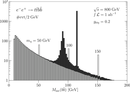
Figure 6: Invariant $b\bar{b}$ mass distribution for $e^{+}e^{-}\to\bar{t}t\bar{b}b$, showing the expected number of events in $2\;{\rm GeV}$ bins for $1\;{\rm ab}^{-1}$ of data. Medium gray is the QCD contribution, dark gray is EW with $m_{H}=115\;{\rm GeV}$. The light-gray spikes are $\eta$ signals for three values of $m_{\eta}$ with $g_{tt\eta}=0.2$. We do not include finite detector resolution effects, so e.g. the $m_{\eta}=150$ GeV signal is marginal.

At an $e^{+}e^{-}$ collider, some models will allow for the possibility of $Z^{*}\to H\eta$, but we do leave this investigation for a later publication [31]. Here we estimate the possibility of producing $\eta$ in $t\bar{t}\eta$ associated production. Unfortunately, even for the analogous $t\bar{t}H$ channel, the cross section is at most a few fb. For $\eta$, the coupling to top quarks $g_{tt\eta}$ is proportional to $v/F$, so the rate is $(v/F)^{2}$-suppressed. On the other hand, the rate is enhanced if $m_{\eta}$ is significantly below $m_{H}$. Fig. 5 shows the total cross section for this process for three choices of $g_{t\bar{t}\eta}$.

In the mass range below $2m_{t}$ the $\eta$ decays with significant BR into a $b\bar{b}$ pair. The most important background is $t\bar{t}b\bar{b}$ production. In Fig. 6 we show the invariant $b\bar{b}$ mass distribution for signal and background, for three choices of $m_{\eta}$ and fixed coupling to top quarks. This plot, which was calculated using the programs of Refs. [35, 36] shows the difficulties in detecting this final state: for low $\eta$ masses, the signal cross section is sizable but the QCD background is rather large. If the $\eta$ mass is close to the $Z$ or Higgs masses, the EW background is oberwhelming. For larger $m_{\eta}$ values which are well separated from the $Z$ and Higgs, the production cross section rapidly decreases. In any case, the experimental analysis of the $t\bar{t}b\bar{b}$ final state is nontrivial [37], and the achievable resolution in the invariant $b\bar{b}$ mass (with correct identification of the $t\bar{t}$ pair) determines the sensitivity for detecting a pseudo-axion in this final state.

In principle, the process $e^{+}e^{-}\to\gamma^{*}\to\eta\gamma$ is possible with the help of the anomaly coupling, but it turns out that the $b\bar{b}\gamma$ background is generally too large for this to be viable.

4.4 Pseudo-axions at a photon collider

Figure 7: Total cross section for resonant $\eta$ production at a future photon collider, with different anomaly coefficients as indicated by the number of non-SM particles with masses $\sim 1\>{\rm TeV}$ in the loop. For comparison, Higgs production cross sections are shown for the SM as well as SM plus a heavy $T$ quark.

Especially for Higgs precision measurements, a high energy photon collider is expected to be operated at a future linear collider, by Compton backscattering laser photons off the electron beam. At such a machine the Higgs boson(s) as well as pseudoscalar Higgs bosons can be produced as $s$-channel resonances [38]. Pseudo-axions could be produced the same way. The effective cross sections for resonant pseudo-axion production with different choices of the anomaly factors (i.e., different numbers of particles in the loop and/or different coupling factors) are shown in Fig. 7. Since all strongly-coupled particles running in the loop are much heavier than the pseudo-axion itself, the cross section remains constant over a wide range of $m_{\eta}$, while the Higgs boson shows the well-known maximum at the $W$ threshold as well as the destructive interference between gauge boson and fermion loops for masses around $650\,{\rm GeV}$.

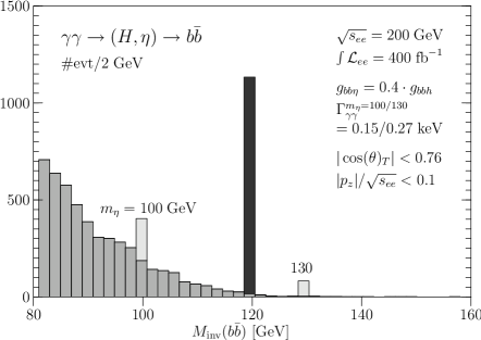
Figure 8: Invariant $b\bar{b}$ mass distribution for $\gamma\gamma\to b\bar{b}$, showing the expected number of events in $2\;{\rm GeV}$ bins for $400\;{\rm fb}^{-1}$ of data. The light gray spikes are $\eta$ signals for various $m_{\eta}$ with $g_{bb\eta}=0.4g_{bbh}$. We also show the SM Higgs signal for $m_{H}=120\;{\rm GeV}$ for comparison (in the $\mu$ model, $m_{H}\sim 420\ldots 440\,{\rm GeV}$). Applied kinematic cuts are shown in the figure. We do not include finite detector resolution effects.

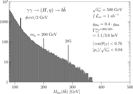
Figure 9: Signals for heavy pseudo-axions at the photon collider for $m_{\eta}=200,285\,{\rm GeV}$. The values for coupling constants and cuts are given in the figure. For comparison, the signal for a $120\,{\rm GeV}$ Higgs is shown (in the $\mu$ model the corresponding Higgs masses in the two cases are $368/230\,{\rm GeV}$, respectively.)

The decay mode $\eta\to b\bar{b}$ is typically large (although not necessarily dominant), and the $\eta$ manifests itself as a sharp spike in the $b\bar{b}$ invariant mass spectrum. Fig. 8 shows the $b\bar{b}$ invariant mass spectrum at a 200 GeV photon collider, which is optimal for studies of a light Higgs boson. Experimentally, the discovery is challenging since the anomaly factor must not be too small and the scale $F$ should not be too high in order for the $\eta$ signal to be clearly visible. For larger $\eta$ masses the situation is almost the same as for the linear collider: the background falls rapidly with increasing $m_{b\bar{b}}$, but the signal cross section falls at a similar rate. Fig. 9 shows the peaks in the $m_{b\bar{b}}$ spectrum for larger $\eta$ masses. For very heavy pseudo-axions, $m_{\eta}\sim 350\,{\rm GeV}$, the $t\bar{t}$ channel opens up and one can look for peaks in this spectrum. Figs. 8 and 9 were produced with the programs of Refs. [39, 40].

Mühlleitner et al. [38] studied the case of a pseudoscalar Higgs boson in a certain region of MSSM parameter space, in which the Higgs pseudoscalar $A$ has exactly the same total width and BR($b\bar{b}$) as the $\mu$ model $\eta$ at the Golden Point. They considered finite $b\bar{b}$ resolution and other effects, such as detector smearing of the signal, and found a significant pseudoscalar signal at the photon collider.

5 Conclusions

If a Little Higgs scenario is realized in nature, Higgs bosons at the EW scale are typically accompanied by new gauge-singlet pseudoscalar particles $\eta$ that are associated with the extra spontaneously broken $U(1)$ symmetry groups. If these abelian subgroups are gauged, the particles are absorbed as the longitudinal components of extra $Z^{\prime}$ bosons. At future colliders, such (heavy) vector resonances can be detected by standard methods. Their indirect effects on the existing EW precision data already constrain the parameter space of Little Higgs models.

Therefore, we have considered the alternative case that at least one $U(1)$ group is ungauged, so that the associated NGB is physical. To avoid the limits on light axions, we require the presence of explicit $U(1)$ symmetry breaking terms which give the would-be axion a mass in the EW range. In particular models, some of the pseudo-axion masses are calculable, while in other models (such as the Littlest Higgs model) $m_{\eta}$ is undetermined.

Detecting these particles would be an important test of the Little Higgs model structure. At the LHC, one can perhaps search for them in decays of the heavy top quark partners $T\to t\eta$ and subsequent decay $\eta\to b\bar{b}$, or possibly $\eta\to gg$ for extreme parameter choices or at an upgraded LHC or a future, higher-energy hadron collider. In some models, the decay $\eta\to ZH$ is open, giving rise to extremely distinctive but probably small signals. In either case, $T\to t\eta$ decay channels are extremely complicated and their exact utility will have to await further detailed work. Our work has been to point out that the presence of pseudo-axions generally alters the phenomenology of $T$ quarks, often significantly and in some cases to the point of domination.

Our much more interesting result is the prospect of searching for pseudo-axions in direct production at hadron colliders, $gg\to\eta$, with subsequent decay to photon pairs, in the spirit of Higgs boson searches. While observation does not appear to generally be possible in the Littlest model without fine-tuned choices of the fermion $U(1)_{\eta}$ charges, in the $\mu$ model the $\eta$ would be visible at the LHC for larger values of $m_{\eta}$, and over significant parameter space at the luminosity-upgraded SLHC. The general feature of direct production is that the more heavy quark partners of the model, the stronger the production rate; e.g. one would expect even larger rates in the Simple Group model. Unlike pseudoscalars in supersymmetry, the BR($\gamma\gamma$) is not suppressed by fermion couplings enhanced by $\tan\beta^{2}$ dominating the total decay width ($\tan\beta$ is typically restricted to large values in supersymmetry scenarios). Instead, in general the $b\bar{b}\eta$ couplings are suppressed relative to Higgs-like couplings, resulting in an often sub-dominant BR relative to the $gg$ final state, and a non-trivial BR($\gamma\gamma$) even up to the $ZH$ or $t\bar{t}$ thresholds.

The production channels at a Linear Collider ($e^{+}e^{-}\to t\bar{t}\eta$) or at a photon collider ($\gamma\gamma\to\eta$) are also promising, and we have presented results for a few cases. While the backgrounds to these processes appear manageable, the expected signal rates are low, so high luminosity and a sophisticated experimental analysis will be necessary to confirm the presence of a low-mass pseudo-axion.

The pseudoscalar’s nature would easily be distinguished from a standard Higgs boson by the absence of the $WW$ and $ZZ$ fusion channels, which are well-known to work over an extremely large mass range [41], as well as “standard” decay channels such as $gg\to\eta\to W^{+}W^{-},ZZ$ [42, 32, 33].

To distinguish $\eta$ from a pseudoscalar Higgs in more conventional two-doublet models or other extended Higgs sectors, we would have to identify it as a gauge singlet. We anticipate that observing all possible $T$ decay modes would aid this, but it probably would require an $e^{+}e^{-}$ collider which can cover the parameter space as well as prove the absence of charged and additional CP-even neutral partners.

Acknowledgements

We thank K. Desch, R. Harlander, G. Hiller, T. Ohl, M. Peskin, and A. Pierce for useful discussions, Martin Schmaltz and Tim Tait for critical reviews of the manuscript, and Thomas Binoth for providing us with Diphox NLO diphoton continuum predictions for the LHC. W.K. is grateful for the hospitality of the SLAC Theory Group, and D.R. thanks the KITP for its hospitality, where part of this work was completed. This research was supported in part by the National Science Foundation under Grant No. PHY99-07949, the U.S. Department of Energy under grant No. DE-FG02-91ER40685, and by the Helmholtz-Gemeinschaft under Grant No. VH-NG-005. J.R. was also supported by the DFG Sonderforschungsbereich (SFB) “Transregio 9 – Computergestützte Theoretische Teilchenphysik” and the Graduiertenkolleg (GK) “Hochenergiephysik und Teilchenastrophysik”.

Appendix A Heavy $T$ quark decay partial widths

In the Littlest Higgs model, the $T$ partial decay widths $T\to tH$ and $T\to t\eta$ are given by

$$\Gamma =\frac{M_{T}}{32\pi}f(x_{t},x_{h})[(1+x_{t}^{2}-x_{h}^{2})(\kappa_{L}^{2}+\kappa_{R}^{2})+4\kappa_{L}\kappa_{R}x_{t}]$$ (50)

with the usual definitions $x_{i}=m_{i}/M_{T}$ and the function

$$f(x_{i},x_{j}) =\sqrt{(1-(x_{i}+x_{j})^{2})(1-(x_{i}-x_{j})^{2})},$$ (51)

where for $H$ and $\eta$ the left- and right-handed couplings are

$$\kappa_{L}^{H} =\mathcal{O}\left(\frac{v}{F}\right) \kappa_{R}^{H} =-\frac{s}{c}\frac{m}{v}$$ (52)

$$\kappa_{L}^{\eta} =i\frac{m}{v}\beta^{\prime} \kappa_{R}^{\eta} =i\mathcal{O}\left(\frac{v}{F}\right)$$ (53)

In the limit $v/F\to 0$ where the masses of $H,Z,W$, and $\eta$ can be neglected compared to $M_{T}$, $SU(2)$ symmetry relates the partial decay widths into (longitudinally polarized) vector bosons to the partial decay widths into a Higgs boson, and the BRs simplify to

$$\Gamma(T\to tH) =\frac{M_{T}}{32\pi}\frac{m^{2}}{v^{2}}\frac{s^{2}}{c^{2}}=\Gamma(T\to tZ^{0})=\frac{1}{2}\Gamma(T\to bW^{+})$$ (54)

$$\Gamma(T\to t\eta) =\frac{M_{T}}{32\pi}\frac{m^{2}}{v^{2}}\beta^{\prime 2}\;.$$ (55)

For the $\mu$ model, the partial widths of the heavy $T$ quark (neglecting the $b$ quark mass) are:

$$\Gamma(T\to th) =\;\frac{M_{T}}{32\pi}f(x_{t},x_{h})\left[(1+x_{t}^{2}-x_{h}^{2})(\kappa_{L}^{h\,2}+\kappa_{R}^{h\,2})+4\kappa_{L}^{h}\kappa_{R}^{h}x_{t}\right]$$ (56)

$$\Gamma(T\to t\eta) =\;\frac{M_{T}}{32\pi}f(x_{t},x_{\eta})\left[(1+x_{t}^{2}-x_{\eta}^{2})(\kappa_{L}^{\eta\,2}+\kappa_{R}^{\eta\,2})+4\kappa_{L}^{\eta}\kappa_{R}^{\eta}x_{t}\right]$$ (57)

$$\Gamma(T\to Zt) =\;\frac{\sqrt{\lambda(M_{T}^{2},m_{Z},m_{t})}}{16\pi M_{T}^{3}}\biggl{\{}(c_{V}^{2}+c_{A}^{2})\Bigl{(}M_{T}^{2}-m_{Z}^{2}+m_{t}^{2}+$$ (58)

$$\qquad\frac{(M_{T}^{2}+m_{Z}^{2}-m_{t}^{2})(M_{T}^{2}-m_{Z}^{2}-m_{t}^{2})}{m_{Z}^{2}}\Bigr{)}-6M_{T}m_{t}(c_{V}^{2}-c_{A}^{2})\biggr{\}}$$ (59)

$$\Gamma(T\to Wb) =\;\frac{\sqrt{\lambda(M_{T}^{2},m_{W}^{2},0)}}{32\pi M_{T}^{3}}g_{TWb}^{2}(M_{T}^{2}-m_{W}^{2})\left(2+\frac{M_{T}^{2}}{m_{W}^{2}}\right)$$ (60)

with

$$\lambda(x,y,z)=(x-(y+z)^{2})(x-(y-z)^{2})\;.$$ (61)

Yukawa-type couplings are defined as

$$\bar{\Psi}\gamma^{\mu}(c_{V}-\gamma^{5}c_{A})\Psi,\qquad g\bar{\Psi}\gamma^{\mu}\frac{1}{2}(1-\gamma^{5})\Psi\;.$$ (62)

Appendix B Loop-induced couplings

Little Higgs pseudo-axions couple to vector bosons at one-loop order via the usual triangle graphs in Higgs phenomenology. All fermions which get their mass by $U(1)_{\eta}$ breaking run in the loop. As long as these fermions are heavy compared to the axion, the loop value is independent of the heavy-fermion mass. It depends only on the triangle anomaly coefficient, i.e., the magnitudes of the effective $\eta\gamma\gamma$, $\eta W^{+}W^{-}$, $\eta ZZ$ and $\eta gg$ vertices, given by the mixed anomalies of the $U(1)_{\eta}$ symmetry with the electromagnetic, EW, and QCD gauge groups, respectively. We write the anomaly coefficients $C_{i}$ as parameters:

$$\begin{split}\mathcal{L}_{\text{anom.}}&=\frac{1}{F}\frac{\alpha_{s}}{8\pi^{2}}C_{g}\cdot\eta G_{\mu\nu}\tilde{G}^{\mu\nu}+\frac{1}{F}\frac{\alpha}{8\pi^{2}}C_{\gamma}\cdot\eta A_{\mu\nu}\tilde{A}^{\mu\nu}\\ &\quad+\frac{1}{F}\frac{\alpha}{4\pi^{2}}C_{Z\gamma}\cdot\eta Z_{\mu\nu}\tilde{A}^{\mu\nu}+\frac{1}{F}\frac{\alpha}{8\pi^{2}}C_{Z}\cdot\eta Z_{\mu\nu}\tilde{Z}^{\mu\nu}+\frac{1}{F}\frac{\alpha}{4\pi^{2}}C_{W}\cdot\eta W^{+}_{\mu\nu}\tilde{W}^{-\,\mu\nu}\end{split}$$ (63)

The dual field strengths are normalized by $\tilde{F}^{\mu\nu}=\frac{1}{2}\epsilon^{\mu\nu\rho\sigma}F_{\rho\sigma}$ The values of the anomaly coefficients are model-dependent and given by

$$C_{\gamma} =\;\sum_{f}N^{f}_{c}Q_{f}^{2}|F^{\eta}_{1/2}(4m_{f}^{2}/m_{\eta}^{2})|\frac{g_{\eta f\bar{f}}}{\lambda_{f}}\,,$$ (64a)

$$C_{g} =\;\sum_{q}\frac{1}{2}\,|F^{\eta}_{1/2}(4m_{q}^{2}/m_{\eta}^{2})|\frac{g_{\eta q\bar{q}}}{\lambda_{q}}\,,$$ (64b)

where the mass of the fermion in the loop is parameterized by $m_{f}=\lambda_{f}F$ (for heavy particles $\lambda_{f}$ and $g_{\eta f\bar{f}}$ are both order one, while for SM particles like the top both are order $v/F$) and $F_{1/2}^{\eta}$ is the function defined in [43]. We are not interested in the operators containing the $W$ or the $Z$ here because the $\eta$ already has small production cross sections, and further small BRs to observable (lepton) final states makes these decays moot. The relevant couplings are given in Eq. (11) for the Littlest Higgs model and in Eq. (23) for the $\mu$ model. Unlike for a Higgs scalar, the $W$ loop is unimportant, since the $\eta$ does not couple to weak bosons at tree level. Since the $W$ loop would otherwise contribute with opposite sign to fermion loops, there is no destructive interference as in the SM.

In contrast, in Little Higgs models the masses of all new heavy fermions are expected to be non-invariant under the $U(1)_{\eta}$ symmetries (to make the model natural), hence they all contribute to the axion-gauge boson interactions with full strength. In particular, the Simple Group models discussed above predict heavy partners for all SM fermions. Leaving aside the detailed coupling structure, for the $\eta gg$ coupling the heavy quark triangle diagram value is approximately multiplied by $N=3$ (the number of quarks) in the $\mu$ model, or $N=6$ in the Simple Group model. For the coupling to EW gauge bosons, the heavy partners of leptons and neutrinos have also to be included in the loop, which we ignore here. Note also that in extended scalar sectors in models like the $[SU(4)/SU(3)]^{4}$ simple group, there can be enhancement effects by the tangent of a mixing angle analogous to that of the MSSM. The loop integrals for the triangle graphs are found in [43].

In the Littlest Higgs model, the situation is less certain since we do not know how many heavy fermions actually exist. Furthermore, we need the absolute $U(1)_{\eta}$ charges of the fermions, while the previously introduced $\beta$ coefficients are merely differences of $U(1)_{\eta}$ charges. Here, we cannot predict the anomaly coefficients but have to leave them as free parameters. It is even possible for them to cancel for randomly chosen integer values of $\beta_{0},\beta_{1},\beta_{2}$. This is largely irrelevant, however, as we note that the normalization factor $1/\sqrt{5}$ squared highly suppresses the anomalous partial widths. This is peculiar to the Littlest Higgs model and is due to the hypercharge embedding. However, judicious choice of the $\beta$ coefficients can compensate for this.

Nevertheless, it is not unreasonable to expect that the factor $v/F$, which suppresses the $\eta$ couplings compared to the corresponding CP-even or CP-odd Higgs couplings in the SM or MSSM, is compensated by the large weight of the heavy-fermion sector in any Little Higgs model.

References

- [1] N. Arkani-Hamed, A. G. Cohen, H. Georgi, Phys. Lett. B 513 (2001) 232; N. Arkani-Hamed, A. G. Cohen, T. Gregoire, and J. G. Wacker, JHEP 0208 (2002) 020.
- [2] E. Katz, J. y. Lee, A. E. Nelson and D. G. E. Walker, arXiv:hep-ph/0312287; M. Piai, A. Pierce and J. Wacker, arXiv:hep-ph/0405242.
- [3] D. E. Kaplan, M. Schmaltz and W. Skiba, arXiv:hep-ph/0405257.
- [4] A. Birkedal, Z. Chacko and M. K. Gaillard, arXiv:hep-ph/0404197; P. H. Chankowski, A. Falkowski, S. Pokorski and J. Wagner, Phys. Lett. B598 (2004) 252.
- [5] N. Arkani-Hamed, A. G. Cohen, E. Katz, and A. E. Nelson, JHEP 0207 (2002) 034.
- [6] N. Arkani-Hamed et al., JHEP 0208 (2002) 021.
- [7] D. E. Kaplan and M. Schmaltz, JHEP 0310 (2003) 039.
- [8] I. Low, W. Skiba, and D. Smith, Phys. Rev. D 66 (2002) 072001. S. Chang and J. G. Wacker, Phys. Rev. D 69 (2004) 035002; T. Gregoire, D. R. Smith, and J. G. Wacker, Phys. Rev. D 69 (2004) 115008; W. Skiba and J. Terning, Phys. Rev. D 68 (2003) 075001; S. Chang, JHEP 0312 (2003) 057.
- [9] M. Schmaltz, JHEP 0408 (2004) 056.
- [10] S. R. Coleman and E. Weinberg, Phys. Rev. D 7 (1973) 1888.
- [11] D. B. Kaplan and H. Georgi, Phys. Lett. B 136 (1984) 183; D. B. Kaplan, H. Georgi and S. Dimopoulos, Phys. Lett. B 136 (1984) 187.
- [12] C. T. Hill, S. Pokorski and J. Wang, Phys. Rev. D 64 (2001) 105005; N. Arkani-Hamed, A. G. Cohen and H. Georgi, Phys. Lett. B 513 (2001) 232.
- [13] C. Csáki et al., Phys. Rev. D 67 (2003) 115002.
- [14] J. L. Hewett, F. J. Petriello, and T. G. Rizzo, JHEP 0310 (2003) 062.
- [15] T. Han, H. E. Logan, B. McElrath, and L.-T. Wang, Phys. Rev. D 67 (2003) 095004.
- [16] C. Csaki et al., Phys. Rev. D 68 (2003) 035009.
- [17] M. Perelstein, M. E. Peskin, and A. Pierce, Phys. Rev. D 69 (2004) 075002.
- [18] S. C. Park and J.-H. Song, arXiv:hep-ph/0306112; M.-C. Chen and S. Dawson, Phys. Rev. D 70 (2004) 015003; R. Casalbuoni, A. Deandrea, and M. Oertel, JHEP 0402 (2004) 032.
- [19] W. Kilian and J. Reuter, Phys. Rev. D 70 (2004) 015004.
- [20] S. Weinberg, Phys. Rev. D 13 (1976) 974; L. Susskind, Phys. Rev. D 20 (1979) 2619; E. Farhi and L. Susskind, Phys. Rev. D 20 (1979) 3404; E. Eichten and K. D. Lane, Phys. Lett. B 90 (1980) 125.
- [21] S. Dimopoulos, Nucl. Phys. B 168 (1980) 69; E. Eichten, I. Hinchliffe, K. D. Lane and C. Quigg, Rev. Mod. Phys. 56 (1984) 579 [Addendum-ibid. 58 (1986) 1065]; E. Eichten, I. Hinchliffe, K. D. Lane and C. Quigg, Phys. Rev. D 34 (1986) 1547; R. Casalbuoni et al., Nucl. Phys. B 555 (1999) 3.
- [22] B. A. Dobrescu and C. T. Hill, Phys. Rev. Lett. 81 (1998) 2634; R. S. Chivukula, B. A. Dobrescu, H. Georgi and C. T. Hill, Phys. Rev. D 59 (1999) 075003; G. Burdman and N. J. Evans, Phys. Rev. D 59 (1999) 115005.
- [23] B. A. Dobrescu, Phys. Rev. D 63 (2001) 015004.
- [24] J. R. Ellis et al., Phys. Rev. D 39 (1989) 844; U. Ellwanger, M. Rausch de Traubenberg and C. A. Savoy, Nucl. Phys. B 492 (1997) 21; D. J. Miller, R. Nevzorov and P. M. Zerwas, Nucl. Phys. B 681 (2004) 3.
- [25] B. A. Dobrescu and K. T. Matchev, JHEP 0009 (2000) 031; G. Hiller, Phys. Rev. D 70 (2004) 034018.
- [26] G. Burdman, M. Perelstein, and A. Pierce, Phys. Rev. Lett. 90 (2003) 241802 [Erratum-ibid. 92 (2004) 049903].
- [27] A. K. Leibovich and D. L. Rainwater, Phys. Rev. D 65, 055012 (2002).
- [28] D. Kominis, Nucl. Phys. B 427, 575 (1994)
- [29] G. Azuelos et al., arXiv:hep-ph/0402037.
- [30] F. Gianotti et al., arXiv:hep-ph/0204087.
- [31] W. Kilian, D. Rainwater and J. Reuter, Phys. Rev. D 74, 095003 (2006) [arXiv:hep-ph/0609119].
- [32] ATLAS TDR, report CERN/LHCC/99-15 (1999).
- [33] CMS TP, report CERN/LHCC/94-38 (1994).
- [34] T. Binoth, J. P. Guillet, E. Pilon and M. Werlen, Eur. Phys. J. C 16 (2000) 311; T. Binoth, J. P. Guillet, E. Pilon and M. Werlen, Eur. Phys. J. directC 4 (2002) 7.
- [35] http://whizard.event-generator.org; W. Kilian, T. Ohl and J. Reuter, arXiv:0708.4233 [hep-ph]; W. Kilian, LC-TOOL-2001-039, Jan 2001.
- [36] T. Stelzer, F. Long, Comput. Phys. Commun. 81 (1994) 357.
- [37] A. Gay, A. Besson, and M. Winter, to appear in: Proc. LCWS 2004, Paris, France.
- [38] M. M. Mühlleitner, M. Krämer, M. Spira and P. M. Zerwas, Phys. Lett. B 508, 311 (2001); [arXiv:hep-ph/0101083]. K. Cheung and H. W. Tseng, arXiv:hep-ph/0410231; J. Tandean, Phys. Rev. D52 (1995) 1398.
- [39] T. Ohl, O’Mega: An Optimizing Matrix Element Generator, in Proceedings of 7th International Workshop on Advanced Computing and Analysis Techniques in Physics Research (ACAT 2000) (Fermilab, Batavia, Il, 2000) [arXiv:hep-ph/0011243]; M. Moretti, T. Ohl, J. Reuter, [arXiv:hep-ph/0102195].
- [40] T. Ohl, Comput. Phys. Commun. 101 (1997) 269; T. Ohl, Circe 2.0 Beam Spectra for Simulating Linear Collider and Photon Collider Physics, WUE-ITP-2002-006.
- [41] S. Asai et al., Eur. Phys. J. C 32S2, 19 (2004).
- [42] M. Dittmar and H. K. Dreiner, Phys. Rev. D 55, 167 (1997).
- [43] J. F. Gunion, H. E. Haber, G. Kane, and S. Dawson, The Higgs Hunter’s Guide, Addison-Wesley Publ. Co., 1990.