${\cal{O}}(\alpha_{s}^{2})$ QCD corrections to the electroproduction of hadrons with high
transverse momentum.

Abstract

We compute the order $\alpha_{s}^{2}$ corrections to the one particle inclusive electroproduction cross section of hadrons with non vanishing transverse momentum. We perform the full calculation analytically, and obtain the expression of the factorized (finite) cross section at this order. We compare our results with H1 data on forward production of $\pi^{0}$, and discuss the phenomenological implications of the rather large higher order contributions obtained in that case. Specifically, we analyze the cross section sensitivity to the factorization and renormalization scales, and to the input fragmentation functions, over the kinematical region covered by data. We conclude that the data is well described by the ${\cal{O}}(\alpha_{s}^{2})$ predictions within the theoretical uncertainties and without the inclusion of any physics content beyond the DGLAP approach.

Introduction

The precise measurement of final state hadrons in lepton nucleon deep inelastic scattering constitutes an excellent benchmark for different features of perturbative quantum chromodynamics (pQCD). These processes are crucially sensitive to the three main ingredients of pQCD: the parton content of the nucleon, the hadronization mechanism of partons into the detected final state hadron, and the parton radiation before and after the interaction with the electromagnetic prove.

The first of these ingredients is well characterized by modern parton distribution functions (PDFs). The knowledge on these distributions have become increasingly precise as a result of two decades of high precision inclusive measurements, and the corresponding QCD analyses, driven by the role of PDFs as inputs for theoretical predictions for any experiment involving initial state hadrons MRST04 ; CTEQ . Although the high degree of accuracy attained by PDFs, less inclusive observables, sensitive to flavor combinations of PDFs other than those relevant in inclusive measurements, improve the insight and provide a further check on the universality of PDFs and on factorization.

The second ingredient is addressed by the so called fragmentation functions (FF), which are rapidly evolving following the path of PDFs, but without attaining yet the refinement of the latter KKP ; kretzer . Most of the data used to determine these distributions, which come essentially from electron-positron annihilation into hadrons, give no information on how the individual quark flavor fragments into hadrons and leave a considerable uncertainty on the gluon density. For these reasons, the NLO analysis of one particle inclusive data is crucial for the extraction of fragmentation functions.

The last ingredient concerns higher order QCD calculations, which have been explored and validated for most processes up to next to leading order (NLO) accuracy, and are currently being extended even beyond that point. For the one particle inclusive processes only very recently there has been progress beyond the leading order (LO) gluon ; quark ; aure ; Fontannaz:2004ev ; Maniatis:2004xk . However, up to now there were no analytic computation of the ${\cal{O}}(\alpha_{s}^{2})$ corrections for the electroproduction of hadrons with non vanishing transverse momentum. The analytic computation of the ${\cal{O}}(\alpha_{s}^{2})$ corrections allows us to check factorization in a direct way, which means that collinear singularities showing up in the partonic cross section factorize into PDFs as required by inclusive deep inelastic scattering, and into FFs for electron-positron annihilation into hadrons. As a consequence of this explicit cancellation, the resulting cross section is finite and can be straightforwardly convoluted with PDFs and FFs in a faster and more stable numerical code, compared to what can be usually obtained in numerical implementations using either the subtraction Maniatis:2004xk or the slicing aure ; Fontannaz:2004ev methods. The analytical result is still sufficiently exclusive and keeps the dependence on the rapidity and the transverse momentum of the produced hadron, allowing a detailed comparison with the experimental data.

In this paper we compute the order $\alpha_{s}^{2}$ corrections to the one particle inclusive leptoproduction cross section of hadrons with non vanishing transverse momentum. We perform the cancellation of collinear singularities analytically, and obtain the full expression of the factorized, and thus finite, cross section at this order. The outline of the paper is as follows: in the next section we summarize the relevant kinematics and details about the phase space integration for the O($\alpha_{s}^{2}$) contributions to the cross section, together with the conventions and notation adopted. In section II we compute the corresponding real and virtual amplitudes, we discuss the nature of the singularities that contribute to them, we analyse the factorization of collinear singularities, and pay special attention to the scale dependence induced in the cross section by this factorization procedure. Section III deals with the phenomenological implications of the new corrections. Specifically, we compare our results with data on forward production of $\pi^{0}$, presented recently by the H1 collaboration, as an example, and evaluate the phenomenological implications of the rather large higher order corrections. Special attention is paid to the cross section sensitivity to the factorization scale choosen, and to the fragmentation functions input as sources of theoretical uncertainties. We also analyze the consequences of the forward pion selection on the LO and NLO underlying partonic processes, finding this kinematical suppression as the main reason for the unusual difference between the LO and NLO estimates. In agreement with the results obtained in aure , we conclude that the data is well described by the pure Dokshitzer-Grivov-Lipatov-Altarelli-Parisi (DGLAP) ${\cal{O}}(\alpha_{s}^{2})$ predictions within the theoretical uncertainties, but without need to appeal to resolved photon contributions, as suggested in Fontannaz:2004ev .

I Kinematics

We begin with the kinematical characterization of the one particle inclusive deep inelastic scattering processes. Since the choice of variables required to deal with the singularity structure of electroproduction is different from those used in both photo-production Aurenche:1983eq ; Gordon:1994wu ; deFlorian:1998fq and electroproduction in the very forward region gluon ; quark , in the following we discuss it in some detail. We consider the process

$$l(l)+P(P)\longrightarrow l^{\prime}(l^{\prime})+h(P_{h})+X,$$ (1)

where a lepton of momentum $l$ scatters off a nucleon of momentum $P$ with a lepton of momentum $l^{\prime}$ and a hadron $h$ of momentum $P_{h}$ tagged in the final state. Omitting target fragmentation at zero transverse momentum, which has been discussed at length in gluon ; quark , the cross section for this process can be written as

$$\frac{d\sigma^{h}}{dx_{B}\,dQ^{2}}=\sum_{i,j,n}\,\int_{0}^{1}d\xi\,\int_{0}^{1}d\zeta\,\int\mbox{dPS}^{(n)}\,\left[f_{i}(\xi)\,D_{h/j}(\zeta)\,\frac{d\sigma^{(n)}_{ij}}{dx_{B}\,dQ^{2}\,\mbox{dPS}^{(n)}}\right]$$ (2)

where $\sigma^{(n)}_{ij}$ is the partonic level cross section corresponding to the process

$$l(l)+i(p_{i})\longrightarrow l^{\prime}(l^{\prime})+j(k_{j})+\mbox{n-1 additional partons}\,,$$ (3)

before renormalization of the coupling constant and factorization of collinear singularities. $f_{i}(\xi)$ and $D_{h/j}(\zeta)$ are the bare parton densities and fragmentation functions, and dPS⁽ⁿ⁾ the $n$-parton phase space. $\xi$ is the proton momentum fraction carried by the parton $i$ and $\zeta$ is the fraction of parton $j$ momentum taken away by the final state hadron. In addition to the usual DIS variables,

$$Q^{2}=-q^{2}=-(l^{\prime}-l)^{2}\,,\;\,\,\,\,\,\,x_{B}=\frac{Q^{2}}{2P\cdot q}\,,\;\,\,\,\,\,\,y_{e}=\frac{P\cdot q}{P\cdot l}\,,\;\,\,\,\,\,\,S_{H}=(P+l)^{2}\,,$$ (4)

we define Mandelstam variables both at parton and at hadron level:

$$s =(q+p_{i})^{2} S =(q+P)^{2}\,,$$ (5)

$$t =-2\,q\cdot k_{j} T =-2\,q\cdot P_{h}\,,$$ (6)

$$u =-2\,p_{i}\cdot k_{j} U =-2\,P\cdot P_{h}\,,$$ (7)

respectively. The above definitions imply

$$s =\xi\,S-Q^{2}\,(1-\xi)\,, t =\frac{T}{\zeta}\,, u =\frac{\xi}{\zeta}\,U\,.$$ (8)

Notice that the $t>0$ ($T>0$) region exists only for $Q^{2}\neq 0$, feature that considerably reduces the integration region in the case of photo-production. The following step is the definition of suitable partonic variables to characterize the phase space. The choice of these variables is critical for the identification and further prescription of collinear singularities in the partonic cross section. We find particularly useful the variables

$$y \equiv-\frac{u}{Q^{2}+s} z\equiv\frac{(Q^{2}+s)(s+t+u)}{s\,(Q^{2}+s+u)}\,,$$ (9)

with $y,z\in[0,1]$. In terms of these partonic variables, the $n$-particle phase space can be factorized as:

$$\mbox{dPS}^{(n)}=\widehat{\mbox{dPS}}^{(n-1)}\,dy\,dz\,,$$ (10)

where $\widehat{\mbox{dPS}}^{(n-1)}$ includes the phase space of the ‘spectator’ partons (those that not fragment into the detected final state hadron) and the corresponding jacobian. For example for $n=3$, in $D=4+\epsilon$ dimensions we have

$$\begin{split}\mbox{dPS}^{(3)}&=\left(\frac{s}{4\,\pi}\right)^{\epsilon}\,\frac{s}{(4\,\pi)^{4}\,\Gamma(1+\epsilon)}\,(1-y)\,z^{\epsilon/2}\,y^{\epsilon/2}(1-y)^{\epsilon}\,(1-z)^{\epsilon/2}\,dy\,dz\\ &\times\sin^{1+\epsilon}\beta_{1}\,\sin^{\epsilon}\beta_{2}\,d\beta_{1}\,d\beta_{2}\,,\end{split}$$ (11)

where $\beta_{1}$ and $\beta_{2}$ are the angles defined by the spectator partons in their center of mass frame. In terms of the factorized phase space, eq.(2) reads

$$\frac{d\sigma^{h}}{dx_{B}\,dQ^{2}}=\sum_{i,j,n}\,\int_{0}^{1}d\xi\,\int_{0}^{1}d\zeta\,\int_{0}^{1}\,dy\,\int_{0}^{1}\,dz\,\left[f_{i}(\xi)\,D_{h/j}(\zeta)\,\frac{d\sigma^{(n)}_{ij}}{dx_{B}\,dQ^{2}\,dy\,dz}\right]\,,$$ (12)

where $d\sigma^{(n)}_{ij}/dx_{B}\,dQ^{2}dy\,dz$ is the partonic cross section already integrated over the spectator partons, and with the adequate normalization. Finally, changing variables from ($\xi$,$\zeta$) to hadronic transverse momentum $p_{T}$ and rapidity $\eta$, defined in the center of mass frame of the proton and the virtual photon, we find

$$\frac{d\sigma^{h}}{dx_{B}\,dQ^{2}\,dp_{T}^{2}\,d\eta}=\sum_{i,j,n}\frac{e^{-\eta}\,\sqrt{S}}{|p_{T}|\,(Q^{2}+S)}\,\int_{e^{\eta}\,\frac{|p_{T}|}{\sqrt{S}}}^{\frac{e^{2\eta}}{1+e^{2\eta}}}\,\frac{dy}{1-y}\int_{0}^{1-\frac{y}{1-y}\,e^{-2\eta}}\,\frac{dz}{1-z}\,\left[f_{i}(\xi)\,D_{h/j}(\zeta)\,\frac{d\sigma^{(n)}_{ij}}{dx_{B}\,dQ^{2}\,dy\,dz}\,\right]\,.$$ (13)

In terms of the hadronic variables, $\xi$ and $\zeta$ are given by

$$\xi =\frac{Q^{2}\,(1-y)\,(1-z)+S\,y\,e^{-2\eta}}{(Q^{2}+S)\,(1-y)\,(1-z)} \zeta=\frac{e^{\eta}|p_{T}|}{\sqrt{S}\,y}\,.$$ (14)

Clearly, the transformation is singular at $y=0$, $y=1$ and $z=1$, however these points are excluded by $|p_{T}|>0$ (notice that $|\eta|$ is bounded from above), as can be seen from the limits in eq. (13). Finally, in order to obtain more compact expressions for the partonic cross sections, it turns out to be convenient to introduce the auxiliary variable

$$\varrho=\frac{x_{B}}{\xi}=\frac{Q^{2}}{Q^{2}+s}\,.$$ (15)

II Order $\alpha_{s}$ and $\alpha_{s}^{2}$ partonic cross sections

The partonic cross sections in eq.(13) are calculated order by order in perturbation theory and are related to the parton-photon squared matrix elements $\overline{H}^{(n)}_{\mu\nu}(i,j)$ for the $i+\gamma\rightarrow j+X$ processes

$$\frac{d\sigma^{(n)}_{ij}}{dx_{B}\,dQ^{2}\,dy\,dz}=\frac{\alpha_{em}^{2}}{e^{2}}\frac{1}{\xi\,x_{B}^{2}\,S_{H}^{2}}\left(Y_{M}(-g^{\mu\nu})+Y_{L}\frac{4x_{B}^{2}}{Q^{2}}P^{\mu}P^{\nu}\right)\sum_{n}\overline{H}^{(n)}_{\mu\nu}(i,j)\,.$$ (16)

Matrix elements are averaged over initial state polarizations, summed over final state polarizations, and integrated over the spectator partons (i.e. integrated over $\widehat{\mbox{dPS}}^{(n-1)}$). $\alpha_{em}$ stands for the fine structure constant and $e$ is the electron charge. Finally, $Y_{M}$ and $Y_{L}$ are the standard kinematic factors for the contributions of each photon polarization and are given by,

$$Y_{M}=\frac{1+(1-y_{e})^{2}}{2\,y_{e}^{2}}\,,\>\>\>Y_{L}=\frac{1+4(1-y_{e})+(1-y_{e})^{2}}{2\,y_{e}^{2}}\,.$$ (17)

The first contribution to the cross section (13) comes from the partonic tensor at order $\alpha_{s}$, as, in the naive parton model (${\cal{O}}(\alpha_{s}^{0})$), final state hadrons can only be produced with $|p_{T}|=0$ in the proton-virtual photon rest frame. At order $\alpha_{s}$, the partonic cross sections have no collinear divergences provided $|p_{T}|>0$. Up to order $\epsilon$, they are given by

$$\begin{split}\frac{d\sigma^{(1)}_{qq}}{dx_{B}\,dQ^{2}\,dy\,dz}=\frac{c_{q}\,C_{\epsilon}}{\xi\,x_{B}^{2}\,S_{H}^{2}}\,C_{F}\,&\Bigg{\{}Y_{M}\,\left[\frac{(\varrho+y)^{2}+2\,(1-\varrho-y)}{\left(1-\varrho\right)\,\left(1-y\right)}\,\left(1+\frac{\epsilon}{2}\,L_{1}\right)+\frac{\epsilon}{2}\frac{{\left(\varrho-y\right)}^{2}}{\left(1-\varrho\right)\,\left(1-y\right)}\right]\\ &+Y_{L}\,\left[2\,\varrho\,y\,\left(1+\frac{\epsilon}{2}\,L_{1}\right)\right]+{\cal O}(\epsilon^{2})\Bigg{\}}\,\delta(z)\,,\end{split}$$ (18)

$$\begin{split}\frac{d\sigma^{(1)}_{qg}}{dx_{B}\,dQ^{2}\,dy\,dz}=\frac{c_{q}\,C_{\epsilon}}{\xi\,x_{B}^{2}\,S_{H}^{2}}\,C_{F}\,&\Bigg{\{}Y_{M}\,\left[\frac{\left(1+(\varrho-y)^{2}\right)}{(1-\varrho)\,y}\,\left(1+\frac{\epsilon}{2}\,L_{1}\right)+\frac{\epsilon}{2}\,\frac{{\left(1-\varrho-y\right)}^{2}}{\left(1-\varrho\right)\,y}\right]\\ &+Y_{L}\,\left[2\,\varrho\,\left(1-y\right)\,\left(1+\frac{\epsilon}{2}\,L_{1}\right)\right]+{\cal O}(\epsilon^{2})\Bigg{\}}\,\delta(z)\,,\end{split}$$ (19)

$$\begin{split}\frac{d\sigma^{(1)}_{gq}}{dx_{B}\,dQ^{2}\,dy\,dz}=\frac{c_{q}\,C_{\epsilon}}{\xi\,x_{B}^{2}\,S_{H}^{2}}\,T_{F}\,&\Bigg{\{}Y_{M}\,\left[\frac{\left(1-2\,\left(1-\varrho\right)\,\varrho-2\,\left(1-y\right)\,y\right)}{\left(1-y\right)\,y}\,\left(1+\frac{\epsilon}{2}\,L_{1}\right)+\epsilon\,\frac{\left(\left(1-\varrho\right)\,\varrho+\left(1-y\right)\,y\right)}{\left(1-y\right)\,y}\right]\\ &+Y_{L}\,\left[4\,\left(1-\varrho\right)\,\varrho\,\left(1+\frac{\epsilon}{2}\,L_{1}\right)-2\,\epsilon\,\left(1-\varrho\right)\,\varrho\right]+{\cal O}(\epsilon^{2})\Bigg{\}}\,\delta(z)\,,\end{split}$$ (20)

where

$$c_{q}=\alpha_{em}^{2}2\pi\,(2+\epsilon)\,e_{q}^{2}\,,\>\>\>\>\>\>\>\>C_{\epsilon}=\frac{\alpha_{s}}{2\pi}\,f_{\Gamma}\left(\frac{Q^{2}}{4\pi\mu^{2}}\right)^{\epsilon/2},\>\>\>\>\>\>\>\>f_{\Gamma}={\frac{\Gamma(1+\epsilon/2)}{\Gamma(1+\epsilon)}}\,$$ (21)

and

$$L_{1}=\log\left(\frac{(1-\varrho)(1-y)y}{\varrho}\right)\,.$$ (22)

At order-$\alpha_{s}^{2}$, the partonic cross sections receive contributions from the following reactions:

$$\begin{array}[]{ll}\mbox{Real contributions}&\left\{\begin{array}[]{lcl}\gamma+q(\bar{q})&\rightarrow&g+g+q(\bar{q})\\ \gamma+q_{i}(\bar{q_{i}})&\rightarrow&q_{i}(\bar{q_{i}})+q_{j}+\bar{q_{j}}\,\,\,\,(i\neq j)\\ \gamma+q_{i}(\bar{q_{i}})&\rightarrow&q_{i}(\bar{q_{i}})+q_{i}+\bar{q_{i}}\\ \gamma+g&\rightarrow&g+q+\bar{q}\end{array}\right.\\ \mbox{Virtual contributions}&\left\{\begin{array}[]{lcl}\gamma+q(\bar{q})&\rightarrow&g+q(\bar{q})\\ \gamma+g&\rightarrow&q+\bar{q}\end{array}\right.\end{array}$$ (23)

where any of the outgoing partons can fragment into the final state hadron $h$. Order $\alpha_{s}$ and $\alpha_{s}^{2}$ contributions in the very forward region and its singularity structure have already discussed in deep in references gluon ; quark . In this section we analyze the $|p_{T}|>0$ region, and examine the nature of the singularities that it involves. These contributions are computed in $d=4+\epsilon$ dimensions, in the Feynman gauge, and considering all the quarks as massless. Algebraic manipulations were performed with the aid of the program Mathematica math and the package Tracer tracer to perform the traces over the Dirac indices.

The order $\alpha_{s}^{2}$ partonic cross sections can be obtained from the corresponding quark and gluon initiated amplitudes as in references gluon ; quark , taking care of the appropriate flavor discrimination. The angular integrations can be performed with the standard techniques ert ; been , taking into account the additional complications of the one particle inclusive case: the necessity of collecting to all orders the potentially singular factors in the three particle final state integrals. For the integrals that are known to all orders in $\epsilon$, this is not a problem, while for those which are only known up to a given order a careful treatment is required. Once the angular integrals are performed, matrix elements are still distributions in three variables, $y$ and $z$ and $\varrho$, regulated by the parameter $\epsilon$.

At variance with the very forward case ($|p_{T}|=0$), where the integration over final states leads to overlapping singularities along various curves in the residual phase space, here the only remaining singularities are found at $z=0$ and thus they can be dealt with the standard method. After combining real and virtual contributions to a given partonic process, the cross section can be written as

$$\frac{d\sigma^{(2)}_{ij}}{dx_{B}\,dQ^{2}\,dy\,dz} = \frac{c_{q}\,C_{\epsilon}^{2}}{\xi\,x_{B}^{2}\,S_{H}^{2}}\,\left\{\frac{1}{\epsilon}\,{\cal{P}}^{(2)}_{1\,ij}(\varrho,y,z)\,+C^{(2)}_{ij}(\varrho,y,z)+{\cal O}(\epsilon)\right\}\,,$$ (24)

where the coefficient of the single poles, ${\cal{P}}^{(2)}_{1\,ij}(\varrho,y,z)$, as well as the finite contributions $C^{(2)}_{ij}(\varrho,y,z)$, include ‘delta’ and ‘plus’ distributions in $z$. The IR double poles present in the individual real and virtual contributions cancel out in the sum, providing the first straightforward check on the angular integration of real amplitudes and the loop integrals in the virtual case. In the real terms, the above mentioned double poles come from the product of a pole arising in the integration over the spectators phase space (i.e. integration over $\beta_{1}$ and $\beta_{2}$ in (11)) and a single pole coming from the expansion of $z^{-1+\epsilon}$ factors. Double poles in the virtual contributions always arise from loop integrals.

The remaining singularities, contributing to the single pole, are of UV and collinear origin. The former are removed by means of coupling constant renormalization, whereas the latter have to be factorized in the redefinition of parton densities and fragmentation functions. The redefinition of parton densities is exactly the same as in totally inclusive DIS whereas fragmentation functions are renormalized as they are in one-particle inclusive electron-positron annihilation. Typical expressions for renormalized parton densities and fragmentation functions, up to order $\alpha_{s}^{2}$ and in the $\overline{MS}$ factorization scheme, can be found, for example, in Refs.zijli and rijken respectively. Factorization of collinear singularities and cancellation of the UV ones, then impose

$${\cal{P}}^{(2)}_{1\,ij}(\varrho,y,z)=2\,(C_{lj}^{(1)}\otimes P^{(0)}_{li}+C_{ik}^{(1)}\otimes P^{(0)}_{jk})-\beta_{0}\,C_{ij}^{(1)}$$ (25)

where the $C_{ik}^{(1)}$ correspond to the finite (${\cal O}(\epsilon^{0})$) terms in the ${\cal{O}}(\alpha_{s})$ partonic cross sections of eqs. (18), (19) and (20). $P_{ij}$ are the standard LO Altarelli-Parisi kernels, and $\otimes$ denotes the appropriate convolution coming from the factorization recipes.

The factorized, and thus finite, partonic cross sections have terms proportional to $\delta(z)$, terms containing ‘plus’ distributions, and purely functional contributions. The logarithmic ‘plus’ contributions have their origin in the multiple emission of soft-gluons and can therefore be predicted by taking the order $\alpha_{s}$ expansion of the corresponding resumed cross-section. For a partonic subprocess initiated by a parton $i$, where a parton $j$ fragments, and with a gluon and a parton $s$ as spectators, $\gamma+i\rightarrow g+j+s$, the result is

$$\left.\frac{d\hat{\sigma}^{(2)}_{ij}}{dx_{B}\,dQ^{2}\,dy\,dz}\right|_{+}=\frac{d\hat{\sigma}^{(1)}_{ij}}{dx_{B}\,dQ^{2}\,dy\,dz}\left[1+\frac{\alpha_{s}}{2\pi}\left(\frac{\mbox{ln}z}{z}\right)_{+}\left(4\,C_{i}+4\,C_{j}-2\,C_{s}\right)\right]$$ (26)

where the general color factor $C_{k}$ corresponds to $C_{F}$ if $k$ is a quark and to $C_{A}$ if it is a gluon. The agreement with this prediction provides a further test on our results.

Since the factorized coefficients get contributions from both the real and virtual process at order $\alpha_{s}^{2}$, together with finite terms coming from the renormalization and factorization procedure, their explicit expressions are considerably long and thus are omitted here .

Notice that the renormalization and factorization processes introduce scale dependent terms in the final cross section which partially cancel the scale dependence induced by the coupling constant, parton densities, and fragmentation functions. The structure of these terms follows that of the factorization contributions in eq.(25).

$$-2\left[C_{lj}^{(1)}\otimes P_{li}\,\,\mbox{ln}\left(\frac{M_{F}^{2}}{Q^{2}}\right)+C_{ik}^{(1)}\otimes P_{jk}\,\,\mbox{ln}\left(\frac{M_{D}^{2}}{Q^{2}}\right)\right]+\beta_{0}C_{ij}^{(1)}\,\,\mbox{ln}\left(\frac{M_{R}^{2}}{Q^{2}}\right)$$ (27)

where $M_{R}$, is the renormalization scale and $M_{F}$ and $M_{D}$ are factorization scale for parton densities and fragmentation functions, respectively.

In order to visualize the magnitude of the higher order corrections, in Figure 1 we show the ratio between the order $\alpha_{s}^{2}$ and $\alpha_{s}$ cross sections for $\pi^{0}$ production (K-factor) as a function of $p_{T}$ for $Q^{2}=200\,\mbox{GeV}^{2}$, integrated over rapidity and for different values of $x_{B}$ in the kinematically allowed range. As input parton densities and fragmentation functions we choose the MRST02 MRST02 and KKP KKP , NLO and LO sets, respectively. In the following we refer to the convolution of ${\cal{O}}(\alpha_{s}^{2})$ cross sections and NLO densities as NLO prediction, whereas ${\cal{O}}(\alpha_{s})$ cross sections convoluted with LO densities define the LO estimate.

Figure 1: K-factor as a function of $p_{T}$.

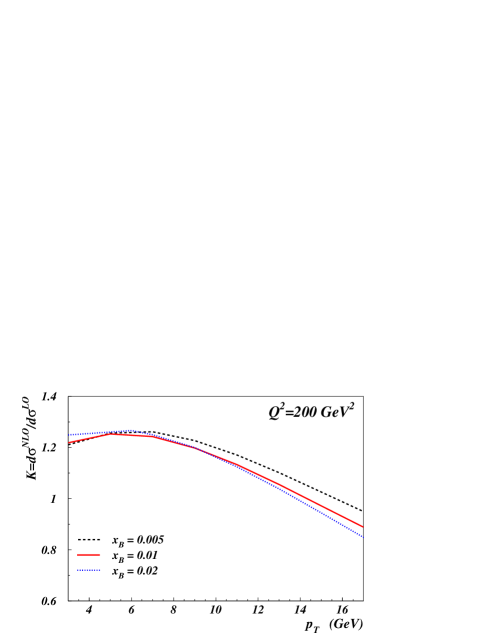
The renormalization and factorization scales $M_{R}^{2}$, $M_{F}^{2}$ and $M_{D}^{2}$ were taken to be the average between the two main physical scales of the process, namely the transverse momentum of the final state particle and the virtuality of the photon as

$$M_{R}^{2}=M_{F}^{2}=M_{D}^{2}=\frac{Q^{2}+p_{T}^{2}}{2}\,.$$ (28)

The K-factor exhibits the characteristic behavior of higher order corrections; they increase at low transverse momentum and also at low $x_{B}$. At very high $p_{T}$, where the LO estimate becomes larger than the NLO prediction, threshold effects become dominant and the perturbative expansion at fixed order in the coupling constant is not expected to be reliable.

The dependence on the particular choice for the factorization and renormalization scales is expected to be weaker at NLO than at LO. In Figure 2 we show this dependence plotting the rate between the cross section evaluated at an arbitrary scale $\mu^{2}$ and the cross section at $\mu^{2}_{0}=(Q^{2}+p_{T}^{2})/2$ as function of the rate $\mu^{2}/\mu^{2}_{0}$.

Figure 2: Scale dependence of the electroproduction cross section.

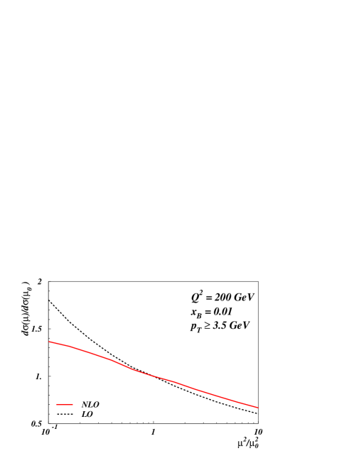
As in the previous plot $Q^{2}=200\,\mbox{GeV}^{2}$, but $x_{B}=0.01$ and we integrate over the allowed $p_{T}$ range, starting from $|p_{T}|>3.5\,\mbox{GeV}$. As expected, the scale dependence is milder for the NLO estimate, although it is not negligible.

Notice that our NLO estimate focus on the ‘direct’ coupling of photons to partons, without taking into account the ‘resolved’ photon contributions, as those computed with virtual photon parton densities. These contributions have been carefully analyzed in references aure ; Fontannaz:2004ev .

III Phenomenology

Recently the H1 Aktas:2004rb collaboration has presented an improved measurement of the production of neutral pions in collisions between $27.6\mbox{ GeV}$ positrons and $820\mbox{ GeV}$ protons. Neutral pions are required to be produced within a small angle $\theta_{\pi}$ from the proton beam in the laboratory frame ($\theta_{\pi}\in[5^{o},25^{o}]$), with an energy fraction $x_{\pi}=E_{\pi}/E_{P}>0.01$ and $2.5<p_{T}<\,15\mbox{ GeV}$. The data confirmed previous measurements which suggested that QCD LO predictions underestimate the cross section at low $x_{B}$ H1viejo . On the other side, predictions based on BFKL dynamics BFKL , or on a large virtual photon content Jung seemed to provide better descriptions.

The disagreement between the H1 data and estimates based on ${\cal{O}}(\alpha_{s})$ cross sections convoluted with LO parton densities and fragmentation functions can be as large as an order of magnitude, depending on the particular kinematical region. This discrepancy is far larger than the typical K-factor found in the previous section, what suggests the onset of a physical mechanism different to leading or next to leading order DGLAP dynamics.

However, several non-negligible effects are present at the particular kinematical regime of the experiment, which are responsible for a large difference between the LO and NLO estimates. The first one is the stringent cut on the pion production angle in H1 data, which suppresses LO and NLO contributions in a different way. The suppression of LO configurations is proportionally bigger than for NLO, implying an effective K-factor much larger than the one found for the cross section without cuts. The second important feature is the rather low value of the scales involved ($p_{T}$ and $Q^{2}$) which enhance the uncertainty due to the particular choice for the factorization scale, even in the NLO calculation, as it has been pointed in aure . This is particularly significant for the lowest $Q^{2}$ bins. Finally, there is also a large uncertainty factor in the theoretical prediction coming from fragmentation functions. Although fragmentation functions reproduce fairly well $e^{+}e^{-}$ annihilation into hadrons, they show large differences when they are used to compute deep inelastic semi-inclusive cross sections.

In Figures 3 and 4 we show the LO and NLO predictions for the electroproduction of neutral pions as a function of $x_{B}$ and $p_{T}$, respectively, in the kinematical range of the H1 experiment, together with the most recent data for the range $p_{T}\geq 3.5\mbox{ GeV}$. The cross sections are computed as described in the previous sections, applying H1 cuts and using MRST02 parton densities MRST02 . Similar results are found using other sets of modern PDFs. For the input fragmentation functions, we use two different sets, the ones from reference KKP denoted as KKP and those from kretzer referenced as K. We set the renormalization and factorization scales as in eq. (27) and we compute $\alpha_{s}$ at NLO(LO) fixing $\Lambda_{QCD}$ as in the MRST analysis, such that $\alpha_{s}(M_{Z})=0.1197(0.130)$.

Figure 3: LO and NLO cross sections, including experimental cuts as explained in the text, as a function of $x_{B}$. H1 data Aktas:2004rb for the range $p_{T}\geq 3.5\mbox{ GeV}$ are also shown.

Figure 4: Cross section as a function of $p_{T}$, data and cuts as in Figure 3.

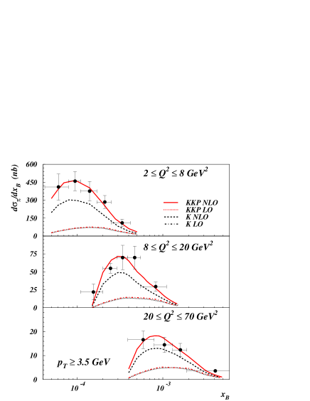
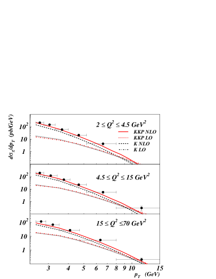
The plots clearly show some of the features mentioned above. On the one hand, the NLO cross sections are much larger than the LO ones, even by the required order of magnitude in certain kinematical regions, once the forward $\pi^{0}$ selection applied by H1 is implemented. The position of the maximum for the $x_{B}$ distribution is also shifted to lower $x_{B}$ values, agreeing nicely with the experimental shape. Cross sections differential in $p_{T}$ show similar features, however the difference between LO and NLO decreases as $p_{T}$ increases.

The uncertainty due to the choice of a fragmentation functions set is also quite noticeable, this fact driven by the different gluon content of the two sets considered here. Low $Q^{2}$ bins seem to prefer KKP set, which have a larger gluon-fragmentation content, whereas for larger $Q^{2}$ both sets agree with the data within errors. LO estimates show a much smaller sensitivity on the choice of fragmentation functions, since gluon fragmentation does not contribute significantly to the cross section at this order.

Figure 5: NLO cross sections as a function of $x_{B}$. The central (solid) line corresponds to setting the factorization and renormalization scales to $(Q^{2}+p_{T}^{2})/2$ and the upper and lower (dashed) ones to $(Q^{2}+p_{T}^{2})/4$ and $Q^{2}+p_{T}^{2}$ respectively.

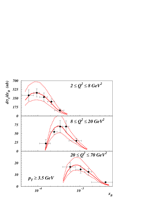
As mentioned, the dependence of the cross section in the choice for the renormalization and factorization scale is also an important source of uncertainty even at NLO. In Figure 5 we show the NLO prediction with the standard choice for the scale, MRST02 parton densities and KKP fragmentation functions (solid line) as in Figure 3, together with H1 data and the estimates with a scale twice as large (lower dashes) and another scale half of the former (upper dashes).

Finally, in order to illustrate the effects of the forward selection criteria, in Figure 6 we show the effective K-factor for the lowest $Q^{2}$ bin, with and without taking into account the constraints on $\theta_{\pi}$ and $x_{\pi}$.

Figure 6: K-factors for the lowest $Q^{2}$ bin of Figure 3 as a function of $x_{B}$ with and without the experimental cuts.

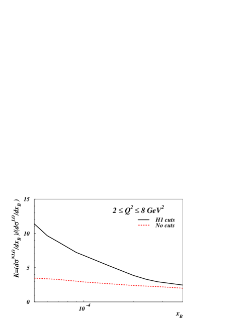
Although the low values of $x_{B}$ and $Q^{2}$ lead to a very large K-factor, the forward selection, typically enhances it by a factor of three. Notice that the process $\gamma+g\rightarrow g+q+\bar{q}$ becomes active at ${\cal{O}}(\alpha_{s}^{2})$ and indeed turns out to be responsible for most of the correction, as it is illustrated in Figure 7, where we show the different contributions to the cross section discriminated by the underlying partonic process.

Figure 7: Contributions to the cross section discriminated by the underlying partonic process for the lowest $Q^{2}$ bin of Figure 3, including experimental cuts. Processes $qg$ and $q\bar{q}$ give negligible contributions and are not shown in the plot.

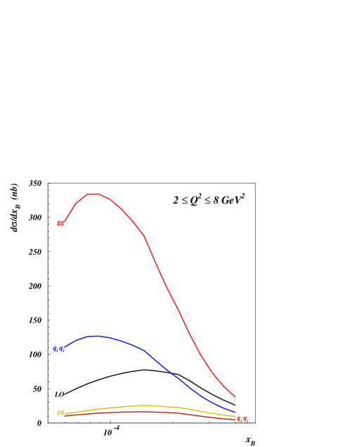
The rather large size of the K-factor can, then, be understood as a consequence of the opening of a new dominant (‘leading-order’) channel, and not to the ‘genuine’ increase in the partonic cross section that might otherwise threaten perturbative stability. The dominance of the new channel is due to the size of the gluon distribution at small $x_{B}$ and to the fact that the H1 selection cuts highlight the kinematical region dominated by the $\gamma+g\rightarrow g+q+\bar{q}$ partonic process. In particular, without the experimental cuts for the final state hadrons, the $gg$ component represents less than $25\%$ of the total NLO contribution at small $x_{B}$, which is dominated by the $gq$ subprocess. The forward selection is also responsible of the scale sensitivity of the cross section, as it supresses large components with small scale dependence whereas it stresses components as $gg$ whose scale dependence would be partly canceled only at NNLO.

IV Conclusions

We have presented the analytical calculation of the differential cross section for semi-inclusive production of a hadron, with non vanishing transverse momentum, in DIS at next-to-leading-order in QCD. As for any semi-inclusive process, the necessity of integrating the phase space of the unobserved particles, but keeping the full dependence on the variables characterizing the final state hadron (and thus of the parton from where it comes), makes the computation of higher order corrections much more involved than the inclusive case. In the present case we showed that, with a suitable parameterization of the phase space, the necessary integrations can be performed analytically and the remaining singularities can be dealt with standard prescription recipes, without the need of substraction or phase space slicing methods.

We found that the order $\alpha_{s}^{2}$ corrections are important, leading to large K-factors. The main contributions to these corrections come from the partonic subprocess $\gamma+g\rightarrow g+q+\bar{q}$ which appears for the first time at that order. The appearance of new channels also leads to quite a significant factorization scale dependence even at the NLO level.

Concerning the phenomenological consequences of our results, we compared them with recent data coming from the H1 experiment at HERA Aktas:2004rb . Within the uncertainties arising from the scale dependence and the particular sensitivity of the results to the gluon hadronization mechanism, parameterized in the fragmentation functions, we found a very good agreement between data and theoretical expectations for both the $x_{B}$ and $p_{T}$ distributions. In particular, fixing the factorization and renormalization scales as just the average between the photon virtuality and the transverse momentum of the final state hadron, both distributions are well described by purely DGLAP evolution. We also found that the experimental cuts applied to the H1 data play a crucial role, boosting the NLO corrections, and thus explaining the unusual poor description of the LO estimate. Finally, our results are in agreement with those obtained previously by numerical methods aure ; Fontannaz:2004ev .

The large K-factors and the significant factorization scale dependence, both related to the opening of new channels at NLO, suggest the presence of non negligible NNLO effects. This feature, altogether with the fact that data is reasonably described by NLO estimates within uncertainties, obliterate any further effect that might contribute, like the resolved component of the photon or those coming from BFKL dynamics in the present experiments.

V Acknowledgements

We warmly acknowledge C. A. García Canal for comments and suggestions. The work of one of us (A.D.) was supported in part by the Swiss National Science Foundation (SNF) through grant No. 200021-101874.

References

- (1) A. D. Martin, R. G. Roberts, W. J. Stirling and R. S. Thorne, arXiv:hep-ph/0411040.
- (2) J. Pumplin, D. R. Stump, J. Huston, H. L. Lai, P. Nadolsky and W. K. Tung, JHEP 0207 (2002) 012 [arXiv:hep-ph/0201195].
- (3) B. A. Kniehl, G. Kramer and B. Potter, Nucl. Phys. B582 (2000) 514 [arXiv:hep-ph/0010289].
- (4) S. Kretzer, Phys. Rev. D62 (2000) 054001. [arXiv:hep-ph/0003177].
- (5) A. Daleo, C. García Canal, R. Sassot, Nucl. Phys. B662 (2003) 334 [arXiv:hep-ph/0303199].
- (6) A. Daleo, R. Sassot, Nucl. Phys. B673 (2003) 357 [arXiv:hep-ph/0309073].
- (7) P. Aurenche, R. Basu, M. Fontannaz and R. M. Godbole, Eur. Phys. J. C34 (2004) 277 [arXiv:hep-ph/0312359].
- (8) M. Fontannaz, arXiv:hep-ph/0410021.
- (9) M. Maniatis, arXiv:hep-ph/0403002.
- (10) P. Aurenche, A. Douiri, R. Baier, M. Fontannaz and D. Schiff, Phys. Lett. B 135 (1984) 164; Nucl. Phys. B 286 (1987) 553.
- (11) L. E. Gordon, Phys. Rev. D 50 (1994) 6753.
- (12) D. de Florian and W. Vogelsang, Phys. Rev. D 57 (1998) 4376 [arXiv:hep-ph/9712273].
- (13) S. Wolfram, Mathematica Third Edition, Cambridge University Press 1996.
- (14) M. Jamin, M.E. Lautenbacher, Comp. Phys. Comm. 74 (1993) 265.
- (15) R. K. Ellis, D. A. Ross and A. E. Terrano, Nucl. Phys. B 178 (1981) 421.
- (16) W. Beenakker, H. Kuijf, W. L. van Neerven and J. Smith, Phys. Rev. D40 (1989) 54. W. Beenakker, Ph. D. Thesis, Leiden, 1989.
- (17) E.B. Zijlstra, W.L. van Neerven, Nuc. Phys. B383 (1992) 525.
- (18) P. J. Rijken, W. L van Neerven, Phys. Lett. B386 (1992) 422.
- (19) A. D. Martin, R. G. Roberts, W. J. Stirling and R. S. Thorne, Eur. Phys. J. C28 (2003) 455 [arXiv:hep-ph/02112080].
- (20) A. Aktas et al. [H1 Collaboration], Eur. Phys. J. C36 (2004) 441 [arXiv:hep-ex/0404009].
- (21) C. Adloff et al. [H1 Collaboration],Phys. Lett. B462 (1999) 440 [arXiv:hep-ex/9907030].
- (22) J. Kwiecinski , A. D. Martin, J. J. Outhwaite, Eur. Phys. J. C9 (1999) 611 [arXiv:hep-ph/9903439].
- (23) H. Jung, L. Jönsson, H. Küster, hep-ph/9805396.