Polarized Structure Functions and the GDH Integral from Lattice QCD

Abstract

The Gerasimov-Drell-Hearn integral $I_{GDH}(Q^{2})$, and its relation to polarized nucleon structure functions, is discussed from the lattice perspective. Of particular interest is the variation of $I_{GDH}(Q^{2})$ with $Q^{2}$, and what it may teach us about the origin and magnitude of higher-twist contributions.

DESY 04-198

1 Introduction

The Gerasimov-Drell-Hearn (GDH) integral, which is written as

$$\begin{split}I_{\rm GDH}(Q^{2})&=\int_{\nu_{0}}^{\infty}\frac{d\nu}{\nu}\left[\sigma^{\stackrel{{\scriptstyle\rightarrow}}{{\Leftarrow}}}(\nu,Q^{2})-\sigma^{\stackrel{{\scriptstyle\rightarrow}}{{\Rightarrow}}}(\nu,Q^{2})\right]\\ &=\frac{8\pi^{2}\alpha}{Q^{2}}\int_{0}^{x_{0}}dx\,\frac{1}{\sqrt{1+\gamma^{2}}}\,\tilde{A}_{1}F_{1}\\ &=\frac{16\pi^{2}\alpha}{Q^{2}}\int_{0}^{x_{0}}dx\,\frac{g_{1}(x,Q^{2})-\gamma^{2}g_{2}(x,Q^{2})}{\sqrt{1+\gamma^{2}}}\,,\end{split}$$ (1)

where $\nu_{0}=m_{\pi}+({m_{\pi}^{2}+Q^{2}})/{2m_{N}}$, $x_{0}={Q^{2}}/{2m_{N}\nu_{0}}$ and $\gamma^{2}={4m_{N}^{2}x^{2}}/{Q^{2}}$, connects the GDH sum rule at $Q^{2}=0$ to the Bjorken and Ellis-Jaffe sum rules at large values of $Q^{2}$. The spin asymmetry $\tilde{A}_{1}$ is known over a large kinematical region for proton, deuterium and helium targets, which allows to compute $I_{\rm GDH}(Q^{2})$ down to $Q^{2}\approx 1$ GeV², separately for the proton and the neutron.

The GDH integral is of phenomenological interest for several reasons. It involves both polarized structure functions of the nucleon, $g_{1}$ and $g_{2}$, and thus tests the spin structure of the proton and the neutron. Furthermore, the GDH integral provides a link between the nucleon state at high and at low resolution, allowing us to study the transition from an assembly of quasi-free partons to strongly coupled quarks and gluons. In particular, we hope to learn about the structure and magnitude of higher-twist contributions. This requires, however, that higher-twist contributions set in gradually and before $Q^{2}$ reaches $\approx$ 1 GeV², that is before the operator product expansion breaks down. In order to match the predictions for $I_{\rm GDH}(0)$, the GDH sum rule, with the Bjorken and Ellis-Jaffe sum rules, a strong variation of $I_{\rm GDH}(Q^{2})$ with increasing $Q^{2}$ is anticipated.

Lattice QCD is in the position to address these questions. In this talk I shall confront measurements of $I_{\rm GDH}(Q^{2})$ with recent lattice results.

2 Polarized Structure Functions

Let me recapitulate what we know about the nucleon’s polarized structure functions $g_{1}$ and $g_{2}$, which enter in (1), first.

A direct theoretical calculation of structure functions is not possible. Using the operator product expansion, we may relate moments of structure functions in a twist or Taylor expansion in $1/Q^{2}$,

$$2\int_{0}^{1}dx\,x^{n}g_{1}(x,Q^{2}) = \frac{1}{2}\,e_{1,n}(Q^{2}/\mu^{2},g(\mu^{2}))\,a_{n}(\mu)+O(1/Q^{2})\,,$$ (2)

$$2\int_{0}^{1}dx\,x^{n}g_{2}(x,Q^{2}) = \frac{n}{2(n+1)}\left[e_{2,n}(Q^{2}/\mu^{2},g(\mu^{2}))\,d_{n}(\mu)\right.$$

$$- \left.e_{1,n}(Q^{2}/\mu^{2},g(\mu^{2}))\,a_{n}(\mu)\right]+O(1/Q^{2})\,,$$

to certain matrix elements of local operators

$$\begin{split}\langle\vec{p},\vec{s}|{\mathcal{O}}^{5}_{\{\sigma\mu_{1}\cdots\mu_{n}\}}|\vec{p},\vec{s}\rangle&=\frac{1}{n+1}a_{n}^{q}\,[s_{\sigma}p_{\mu_{1}}\cdots p_{\mu_{n}}+\cdots-\mbox{traces}]\,,\\[5.0pt] \langle\vec{p},\vec{s}|{\mathcal{O}}^{5}_{[\sigma\{\mu_{1}]\cdots\mu_{n}\}}|\vec{p},\vec{s}\rangle&=\frac{1}{n+1}d_{n}^{\,q}\,[(s_{\sigma}p_{\mu_{1}}-s_{\mu_{1}}p_{\sigma})p_{\mu_{2}}\cdots p_{\mu_{n}}\\ &\hskip 109.54327pt+\cdots-\mbox{traces}]\,,\end{split}$$ (4)

where

$${\mathcal{O}}^{5}_{\sigma\mu_{1}\cdots\mu_{n}}=\left(\frac{i}{2}\right)^{n}\bar{q}\gamma_{\sigma}\gamma_{5}\mbox{\parbox[b]{0.0pt}{$D$}\raisebox{7.3194pt}{$\leftrightarrow$}}_{\mu_{1}}\cdots\mbox{\parbox[b]{0.0pt}{$D$}\raisebox{7.3194pt}{$\leftrightarrow$}}_{\mu_{n}}q-\mbox{traces}\,.$$ (5)

In parton model language

$$\vspace*{0.25cm}a_{n}^{q}=2\int_{0}^{1}dx\,x^{n}\large[\raisebox{-9.95863pt}{$\underbrace{\raisebox{9.95863pt}{$q_{\uparrow}(x,\mu^{2})-q_{\downarrow}(x,\mu^{2})$}}$}\large]=2\Delta^{n}q\,,$$ (6)

$\Delta q(x,\mu^{2})$

in particular $a_{0}^{u}=2\Delta u$, $a_{0}^{d}=2\Delta d$, while $d_{n}^{q}$ has twist three and no parton model interpretation.

In the following I will restrict myself to nonsinglet and valence quark distributions due to lack of space. These quantities show little difference between quenched and full QCD calculations, so that I can further restrict myself to quenched results.

Let us first look at the structure function $g_{1}$. In Table 1 I compare the lattice results for the lower moments of $\Delta q(x,Q^{2})$ [1] with the corresponding phenomenological (experimental) numbers [2]. The quoted result for $\Delta u-\Delta d\equiv g_{A}$ has been taken from a recent, ‘proper’ extrapolation to the chiral limit [3], shown in Fig. 1. By and large we find good agreement.

Let us next look at the structure function $g_{2}$. This differs from $g_{1}$ by twist-three contributions. From (2) we readily see that $g_{2}$ fulfills the Burkhardt-Cottingham sum rule

$$\int_{0}^{1}dx\,g_{2}(x,Q^{2})=0\,.$$ (7)

Moment Lattice [1] Experiment [2]

$$\Delta u_{v}$$

Table 1. Comparison of lattice and experimental values of the lower moments of $\Delta q(x,Q^{2})$, defined in (6), in the $\overline{MS}$ scheme at $Q^{2}=4$ GeV². The subscript $v$ refers to valence quarks.

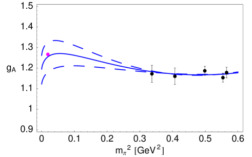
Figure 1: The axial coupling $g_{A}$ as a function of $m_{\pi}^{2}$ together with a fit from chiral perturbation theory.

The first nontrivial moment of the twist-three contribution, $d_{1}^{q}$, can be related to the tensor charge $\delta q$ of the nucleon [4],

$$\begin{split}d_{1}^{\,q}\,(s_{\mu}p_{\nu}-s_{\nu}p_{\mu})&=\langle\vec{p},\vec{s}|\bar{q}\!\left(\gamma_{\mu}\gamma_{5}\,\mbox{\parbox[b]{0.0pt}{$D$}\raisebox{7.3194pt}{$\leftrightarrow$}}_{\!\nu}-\mbox{\parbox[b]{0.0pt}{$D$}\raisebox{7.3194pt}{$\leftrightarrow$}}_{\!\mu}\gamma_{\nu}\gamma_{5}\right)\!q|\vec{p},\vec{s}\rangle\\[3.22916pt] &=-\frac{i}{2}\,\langle\vec{p},\vec{s}|\bar{q}\!\left(\sigma_{\mu\nu}\gamma_{5}\,\mbox{\parbox[b]{0.0pt}{$\not{D}$}\raisebox{7.3194pt}{$\rightarrow$}}+\mbox{\parbox[b]{0.0pt}{$\not{D}$}\raisebox{7.3194pt}{$\leftarrow$}}\sigma_{\mu\nu}\gamma_{5}\right)\!q|\vec{p},\vec{s}\rangle\\[3.22916pt] &=i\,m_{q}\,\langle\vec{p},\vec{s}|\bar{q}\sigma_{\mu\nu}\gamma_{5}q|\vec{p},\vec{s}\rangle\\[3.22916pt] &=\frac{2m_{q}}{m_{N}}\,\delta q\,(s_{\mu}p_{\nu}-s_{\nu}p_{\mu})\,,\end{split}$$ (8)

where $m_{q}$ is the mass of the quark. Thus we have

$$d_{1}^{q}(Q^{2})=\frac{2m_{q}}{m_{N}}\delta q(Q^{2})\,,$$ (9)

which vanishes in the chiral limit ($m_{q}\rightarrow 0$). The second moment, $d_{2}^{q}$, has been computed on the lattice [5]. The result is shown in Fig. 2, separately for the proton and the neutron, and found to be in good agreement with experiment [6]. From (2) and (2) we obtain

$$\int_{0}^{1}dx\,x^{2}g_{2}(x,Q^{2})+\frac{2}{3}\int_{0}^{1}dx\,x^{2}g_{1}(x,Q^{2})=\frac{1}{6}d_{2}\,.$$ (10)

Given the fact that $d_{2}$ is small, and $d_{1}$ even vanishes in the chiral limit, we derive that the Wandzura-Wilczek relation [7]

$$\int_{0}^{1}dx\,x^{n}g_{2}(x,Q^{2}) = -\frac{n}{n+1}\int_{0}^{1}dx\,x^{n}g_{1}(x,Q^{2})\,,$$ (11)

$$g_{2}(x,Q^{2}) = \int_{x}^{1}\frac{dy}{y}\,g_{1}(y,Q^{2})-g_{1}(x,Q^{2})$$ (12)

holds to better than $O(5\%)$, except perhaps at very large $x$, which we are not interested in here. It is needless to say that $g_{2}$ in (12) satisfies the Burkhardt-Cottingham sum rule as well. The structure function $g_{1}(x,Q^{2})$ is obtained from the parton distributions $\Delta q(x,Q^{2})$ by

$$g_{1}(x,Q^{2})=\frac{1}{2}\sum_{q}e_{q}^{2}\int_{x}^{1}\frac{dy}{y}\,e_{1}(y,Q^{2})\,\Delta q\left(\frac{x}{y},Q^{2}\right)$$ (13)

with

$$\int_{0}^{1}dy\,y^{n}e_{1}(y,Q^{2})=e_{1,n}(1,g(Q^{2}))\,.$$ (14)

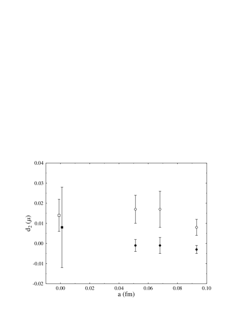
Figure 2: The twist-three contribution $d_{2}(\mu)$ at $\mu^{2}=5$ GeV² for proton ($\Circle$) and neutron ($\CIRCLE$) plotted against the lattice spacing $a$, together with the experimental numbers for proton ($\Box$) and neutron ($\blacksquare$).

3 Higher-Twist Contributions

Contributions of twist four (and higher) have been studied on the lattice, either through calculations of appropriate nucleon matrix elements [8], or by evaluating the operator product expansion directly on the lattice [9]. Higher-twist contributions are generally found to be small. Four-fermion operators, for example, schematically drawn in Fig. 3, which account for diquark effects in the nucleon, contribute

$$\int_{0}^{1}dx\,F_{2}^{(4)}(x,Q^{2})\big{|}_{{\bf 27},I=1}=-0.0005(5)\,\alpha_{s}(Q^{2})\,\frac{m_{N}^{2}}{Q^{2}}\,.$$ (15)

The reason for quoting the flavor 27-plet structure function here, rather than the nucleon (octet) one, is that the underlying four-fermion operator does not mix with operators of lower dimension, which makes it a clean prediction.

Figure 3: Diagrams involving four-fermion operators.

4 The GDH Integral

We are ready now to address the GDH integral. Following our previous discussion, we may assume that higher-twist contributions are small, and that the nucleon’s second polarized structure function $g_{2}$ is well approximated by the Wandzura-Wilczek form (12). Moreover, given the fact that the lattice predictions for $a_{n}^{q}$, compiled in Table 1, are in good agreement with the phenomenological numbers quoted, we may base our further discussion on the parameterization of $g_{1}(x,Q^{2})$ given in Ref. 2.

As already mentioned, I will restrict myself to the nonsinglet GDH integral, which corresponds to proton minus neutron target. In Fig. 4 I show recent results from the Hermes collaboration [10]. I compare this result with the theoretical predictions. The solid line represents the full integral, as given by the bottom line of (1), including $g_{1}$ and $g_{2}$, while the dashed line represents the integral

$$\frac{16\pi^{2}\alpha}{Q^{2}}\int_{0}^{1}dx\,g_{1}(x,Q^{2})\equiv\frac{16\pi^{2}\alpha}{Q^{2}}\Gamma_{1}\,.$$ (16)

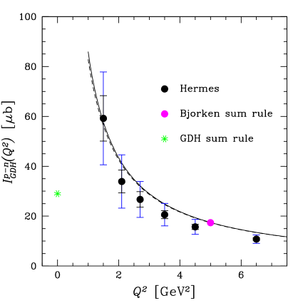
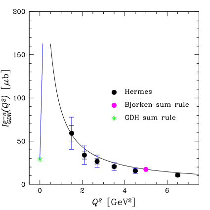
Figure 4: The GDH integral: Experiment versus theory. The inner error bars are statistical, the outer ones statistical plus systematic.

Figure 5: The GDH integral: The connection to the GDH sum rule. The left curve is the prediction of chiral perturbation theory.

Equation (16) corresponds to the limiting case $x_{0}=1$ and $\gamma=0$. The dashed curve can hardly be distinguished from the solid curve over the whole kinematical range, $1\lesssim Q^{2}\leq\infty$, which tells us that the (nonsinglet) GDH integral is insensitive to $g_{2}$ and merely tests the Bjorken sum rule

$$\begin{split}\Gamma_{1}=\int_{0}^{1}dx\,g_{1}(x,Q^{2})&=\frac{1}{6}g_{A}\left[1-\frac{\alpha_{s}(Q^{2})}{\pi}-3.58\,\left(\frac{\alpha_{s}(Q^{2})}{\pi}\right)^{2}\right.\\ &-20.22\,\left.\left(\frac{\alpha_{s}(Q^{2})}{\pi}\right)^{3}+\cdots\right]\,.\end{split}$$ (17)

At larger values of $Q^{2}$ the data fall below the curve. This may be due to the fact that the $x$ range covered shrinks to $0.2\leq x\leq 0.8$ in the highest-$Q^{2}$ bin. In order to draw quantitative conclusions, one certainly would need more precise data. So far we can only say that the experimental data are consistent with leading-twist parton distributions all the way down to $Q^{2}\approx 1$ GeV², and with the Bjorken sum rule in particular.

In Fig. 5 I show the same figure on an enhanced scale, together with the predictions of chiral perturbation theory [11] and the predicted value of the GDH sume rule. Both curves appear to meet in a sharp peak at $Q^{2}\approx 0.4$ GeV². This value lies much below the range of validity of the operator product expansion. Likewise it lies beyond the applicability of chiral perturbation theory, so that no firm statement about the transition from large $Q^{2}$ to the resonance region can be made.

5 Conclusions

To learn anything new, if possible at all, from the GDH integral, we need better experimental data. At present the GDH integral does not teach us anything quantitative about higher-twist contributions. Lattice calculations, on the other hand, indicate that the GDH integral is well represented by the Bjorken sum rule down to $Q^{2}\approx 1$ GeV². More precise lattice data on moments of $g_{1}$ and $g_{2}$, including sea quark effects, will become available soon [12]. In order to match scaling and resonance region, it appears that one will have to resort to model building.

References

- [1] M. Göckeler, R. Horsley, E.-M. Ilgenfritz, H. Perlt, P. Rakow, G. Schierholz and A. Schiller, Phys. Rev. D53, 2317 (1996); M. Göckeler, R. Horsley, L. Mankiewicz, H. Perlt, P. Rakow, G. Schierholz and A. Schiller, Phys. Lett. B414, 340 (1997); S. Capitani, M. Göckeler, R. Horsley, H. Perlt, D. Petters, D. Pleiter, P.E.L. Rakow, G. Schierholz, A. Schiller and P. Stephenson, Nucl. Phys. Proc. Suppl. 79, 548 (1999); M. Göckeler, R. Horsley, W. Kürzinger, H. Oelrich, D. Pleiter, P.E.L. Rakow, A. Schäfer and G. Schierholz, Phys. Rev. D63, 074506 (2001); M. Göckeler et al., in preparation.
- [2] J. Blümlein and H. Böttcher, Nucl. Phys. B636, 225 (2002).
- [3] T.R. Hemmert, M. Procura and W. Weise, Phys. Rev. D68, 075009 (2003).
- [4] This derivation is due to Paul Rakow. Equation (9) is still to be verified numerically.
- [5] Last reference in Ref. 1.
- [6] P.L. Anthony et al. [E155 Collaboration], Phys. Lett. B458, 529 (1999).
- [7] S. Wandzura and F. Wilczek, Phys. Lett. B72, 195 (1977).
- [8] M. Göckeler, R. Horsley, B. Klaus, D. Pleiter, P.E.L. Rakow, S. Schaefer, A. Schäfer and G. Schierholz, Nucl. Phys. B623, 287 (2002).
- [9] S. Capitani, M. Göckeler, R. Horsley, H. Oelrich, D. Petters, P. Rakow and G. Schierholz, Nucl. Phys. Proc. Suppl. 73, 288 (1999).
- [10] A. Airapetian et al. [Hermes Collaboration], Eur. Phys. J. C26, 527 (2003).
- [11] V. Bernard, T.R. Hemmert and U.G. Meissner, Phys. Lett. B545, 105 (2002).
- [12] M. Göckeler et al., in preparation.