OUTP-0422P
TUM-HEP-566/04
SISSA 81/2004/EP
hep-ph/0411190 A Flavor Symmetry for quasi-degenerate Neutrinos: $L_{\mu}-L_{\tau}$

Abstract

We consider the flavor symmetry $L_{\mu}-L_{\tau}$ for the neutrino mass matrix. The most general neutrino mass matrix conserving $L_{\mu}-L_{\tau}$ predicts quasi–degenerate neutrino masses with one maximal and two zero mixing angles. The presence of $L_{\mu}-L_{\tau}$ can also be motivated by the near–bimaximal form of the neutrino mixing matrix. Furthermore, it is a special case of $\mu\tau$ symmetric mass matrices. Breaking the flavor symmetry by adding a small flavor–blind term to the neutrino mass matrix and/or by applying radiative corrections is shown to reproduce the observed neutrino oscillation phenomenology. Both the normal and inverted mass ordering can be accommodated within this scheme. Moderate cancellation for neutrinoless double beta decay is expected. The observables $|U_{e3}|^{2}$ and $|1/2-\sin^{2}\theta_{23}|$ are proportional to the inverse of the fourth power of the common neutrino mass scale. We comment on whether the atmospheric neutrino mixing is expected to lie above or below $\pi/4$. We finally present a model based on the see–saw mechanism which generates a light neutrino mass matrix with an (approximate) $L_{\mu}-L_{\tau}$ flavor symmetry. This is a minimal model with just one standard Higgs doublet and three heavy right–handed neutrinos. It needs only small values for the soft $L_{\mu}-L_{\tau}$ breaking terms to reproduce the phenomenological viable mass textures analyzed.

1 Introduction

The structure of the neutrino mixing matrix is seen to be remarkably different from the quark mixing matrix. Within the standard parametrization of the PMNS [1] mixing matrix

$$\begin{array}[]{c}U=\left(\begin{array}[]{ccc}c_{12}c_{13}&s_{12}c_{13}&s_{13}\\[5.69046pt] -s_{12}c_{23}-c_{12}s_{23}s_{13}&c_{12}c_{23}-s_{12}s_{23}s_{13}&s_{23}c_{13}\\[5.69046pt] s_{12}s_{23}-c_{12}c_{23}s_{13}&-c_{12}s_{23}-s_{12}c_{23}s_{13}&c_{23}c_{13}\\ \end{array}\right)\,,\end{array}$$ (1)

where $c_{ij}=\cos\theta_{ij}$, $s_{ij}=\sin\theta_{ij}$ and the three physical phases were omitted, the following results emerged:

• a small and possibly zero $\theta_{13}\simeq U_{e3}$ obtained from the results of the CHOOZ and Palo Verde experiments [2];

• a very large and possibly maximal $\theta_{23}$ associated with a mass–squared difference $\mbox{$\Delta m^{2}_{\rm A}$}\simeq 2\cdot 10^{-3}$ eV² needed to explain the atmospheric neutrino data [3] and data from the K2K long baseline accelerator experiment [4];

• a large but non–maximal $\theta_{12}$ associated with a mass–squared scale $\mbox{$\Delta m^{2}_{\odot}$}\simeq 8\cdot 10^{-5}$ eV² coming from the results on solar neutrinos [5] and the KamLAND reactor antineutrino experiment [6].

This mixing structure has to be contrasted with the CKM matrix, whose structure is given in zeroth order by the unit matrix.

In this letter we will consider the possibility that the unusual and unexpected structure of neutrino mixing is the consequence of a flavor symmetry acting on the neutrino mass matrix. In the basis in which the charged lepton mass matrix is real and diagonal, the neutrino mass matrix is defined as

$$m_{\nu}=U\,m_{\nu}^{\rm diag}\,U^{T}~{},$$ (2)

where $m_{\nu}^{\rm diag}$ is a diagonal matrix containing the three neutrino masses $m_{1,2,3}$, for which the normal and inverted mass ordering are allowed. Those two possibilities correspond to $m_{3}>m_{2}>m_{1}$ and $m_{2}>m_{1}>m_{3}$, respectively. The fact that $\mbox{$\Delta m^{2}_{\rm A}$}\gg\mbox{$\Delta m^{2}_{\odot}$}$, together with the limit on neutrino masses of order eV [7], implies that three extreme kinds of mass spectra are possible:

$$\begin{array}[]{cc}\mbox{ normal hierarchy:}&|m_{3}|\simeq\sqrt{\mbox{$\Delta m^{2}_{\rm A}$}}\gg|m_{2}|\simeq\sqrt{\mbox{$\Delta m^{2}_{\odot}$}}\gg|m_{1}|~{},\\[8.5359pt] \mbox{ inverted hierarchy:}&|m_{2}|\simeq|m_{1}|\simeq\sqrt{\mbox{$\Delta m^{2}_{\rm A}$}}\gg|m_{3}|~{},\\[8.5359pt] \mbox{ quasi--degeneracy:}&m_{0}\equiv|m_{3}|\simeq|m_{2}|\simeq|m_{1}|\gg\sqrt{\mbox{$\Delta m^{2}_{\rm A}$}}~{}.\end{array}$$ (3)

The specific flavor symmetry we consider in this paper is $L_{\mu}-L_{\tau}$ which gives rise to a quasi–degenerate spectrum. In general, a matrix strictly conserving $L_{\mu}-L_{\tau}$ will have the form

$$m_{\nu}=m_{0}\left(\begin{array}[]{ccc}c&0&0\\[8.5359pt] \cdot&0&s\\[8.5359pt] \cdot&\cdot&0\end{array}\right)~{},$$ (4)

with a common scale $m_{0}$, $c=\cos\theta$ and $s=\sin\theta$. The matrix which diagonalizes $m_{\nu}$ is given by

$$U=\left(\begin{array}[]{ccc}1&0&0\\[8.5359pt] 0&\sqrt{\frac{1}{2}}&\sqrt{\frac{1}{2}}\\[8.5359pt] 0&-\sqrt{\frac{1}{2}}&\sqrt{\frac{1}{2}}\end{array}\right)~{},$$ (5)

independent of $\theta$. The mass eigenvalues are $c~{}m_{0}$ and $\pm s~{}m_{0}$. We see that for values of $\theta$ far from 0 or $\pi/2$, the three mass eigenstates are of the same order. Thus we obtain a quasi–degenerate neutrino mass scheme. This mass scheme is expected to be more easily testable than the hierarchical ones. Furthermore, we already have one maximal mixing angle, which can be identified with the atmospheric angle $\theta_{23}$ whose value is experimentally known to be close to maximal. Moreover, we also have one zero mixing which is compatible with the experimental upper limit on $\theta_{13}$. The third mixing angle, which is the solar mixing angle $\theta_{12}$, comes out to be zero. This of course is in conflict with the current data from solar and KamLAND experiments. We shall see later that the non–zero value of $\theta_{12}$ could be associated with order one numbers stemming from the breaking of the flavor symmetry under consideration.

We can also motivate the choice of $L_{\mu}-L_{\tau}$ flavor symmetry starting from an assumed bimaximal structure for the neutrino mixing. The experimentally observed “bi–large” structure of the mixing matrix can lead one to assume the bimaximal neutrino mixing scheme [10] as a zeroth order approximation. Various proposals [11, 12, 13] have been made in the literature to deviate the mixing from bimaximal in order to reproduce the observed phenomenology. Bimaximal mixing corresponds to $\theta_{12}=\theta_{23}=\pi/4$ and $\theta_{13}=0$. Hence,

$$U^{\rm bimax}=\left(\begin{array}[]{ccc}\frac{1}{\sqrt{2}}&\frac{1}{\sqrt{2}}&0\\[8.5359pt] -\frac{1}{2}&\frac{1}{2}&\frac{1}{\sqrt{2}}\\[8.5359pt] \frac{1}{2}&-\frac{1}{2}&\frac{1}{\sqrt{2}}\\[8.5359pt] \end{array}\right)~{}.$$ (6)

For bimaximal mixing the following mass matrix is implied:

$$\begin{array}[]{c}m_{\nu}=\left(\begin{array}[]{ccc}\displaystyle A&B&-B\\[5.69046pt] \displaystyle\cdot&\displaystyle D+\frac{A}{2}&\displaystyle D-\frac{A}{2}\\[8.5359pt] \displaystyle\cdot&\cdot&\displaystyle D+\frac{A}{2}\end{array}\right)~{},\end{array}$$ (7)

where

$$A=\frac{m_{1}+m_{2}}{2}~{},~{}B=\frac{m_{2}-m_{1}}{2\,\sqrt{2}}~{},~{}D=\frac{m_{3}}{2}~{}.$$ (8)

In case of leptonic $CP$ conservation, different relative signs for the mass states are possible. We can derive now three very interesting special cases of the matrix Eq. (7), obtained for the three extreme mass hierarchies mentioned above:

• For normal hierarchy, i.e., $m_{3}\gg m_{2,1}$ we have

  $$\begin{array}[]{c}m_{\nu}\simeq\displaystyle\frac{\sqrt{\mbox{$\Delta m^{2}_{\rm A}$}}}{2}\,\left(\begin{array}[]{ccc}\displaystyle 0&0&0\\[5.69046pt] \displaystyle\cdot&\displaystyle 1&\displaystyle 1\\[8.5359pt] \displaystyle\cdot&\cdot&\displaystyle 1\end{array}\right)~{}.\end{array}$$ (9)

  This matrix conserves the flavor symmetry $L_{e}$. It displays the well–known “leading $\mu\tau$ block” [14] structure and produces (similar to the $L_{\mu}-L_{\tau}$ case) maximal mixing in the 23 sector and zero mixing in the 12 and 13 sector. The zero entries are filled with terms of order $\sqrt{R}\equiv\sqrt{\mbox{$\Delta m^{2}_{\odot}$}/\mbox{$\Delta m^{2}_{\rm A}$}}$ once $m_{2}$ is no longer neglected with respect to $m_{3}$. Note that the determinant of the $\mu\tau$ block has then to be small in order to generate large 12 mixing.

• For inverted hierarchy and $m_{2}=-m_{1}$ we find

  $$m_{\nu}=\sqrt{\frac{\mbox{$\Delta m^{2}_{\rm A}$}}{2}}\,\begin{array}[]{c}\left(\begin{array}[]{ccc}0&1&-1\\[8.5359pt] \cdot&0&0\\[8.5359pt] \cdot&\cdot&0\end{array}\right)~{}.\end{array}$$ (10)

  This mass matrix conserves the lepton charge $L_{e}-L_{\mu}-L_{\tau}$ [15, 12, 13, 16] and has been considered by many authors. Note that it generates exact bimaximal mixing.

• For quasi–degenerate neutrinos, on which we will focus in this letter, if we have $m_{1}=m_{2}=-m_{3}$, we get

  $$m_{\nu}=m_{0}\left(\begin{array}[]{ccc}1&0&0\\[8.5359pt] \cdot&0&-1\\[8.5359pt] \cdot&\cdot&0\end{array}\right)~{}.$$ (11)

  This matrix is a special case of the matrix Eq. (4) conserving the lepton charge $L_{\mu}-L_{\tau}$ and generates maximal mixing in the 23 sector and zero mixing in the 12 and 13 sectors. The matrix (11) has been considered in very few papers in the literature — for instance in [17, 18], or more recently in the framework of an $A_{4}$ symmetry in [19]. In this respect, it has also been shown that the flavor symmetry $L_{\mu}-L_{\tau}$ is (in the Standard Model (SM)) anomaly free and may be gauged [20]. To be precise, either $L_{\tau}-L_{e}$, $L_{e}-L_{\mu}$ or $L_{\mu}-L_{\tau}$ can be chosen to be gauged. As argued here, $L_{\mu}-L_{\tau}$ emerges as the phenomenologically most viable candidate among the three possibilities.

In general there are 9 possible Abelian flavor symmetries for three active neutrinos: $L_{e}$, $L_{\mu}$, $L_{\tau}$ using only one flavor; $L_{e}-L_{\mu}$, $L_{e}-L_{\tau}$ and $L_{\mu}-L_{\tau}$ using two flavors; $L_{e}-L_{\mu}-L_{\tau}$, $L_{e}+L_{\mu}-L_{\tau}$ and $L_{e}-L_{\mu}+L_{\tau}$ using three flavors. We have shown that among these 9 candidates, bimaximal neutrino mixing as a zeroth order approximation selects three of them: $L_{e}$ (normal hierarchy), $L_{e}-L_{\mu}-L_{\tau}$ (inverted hierarchy) and $L_{\mu}-L_{\tau}$ (quasi–degeneracy).

The $L_{e}-L_{\mu}-L_{\tau}$ ($L_{e}$) flavor symmetry is often argued as the Abelian symmetry of the underlying theory which produces inverted (normal) hierarchy. Along the same lines, we champion here the case of $L_{\mu}-L_{\tau}$ as the underlying symmetry of the theory which generates a quasi–degenerate spectrum for the neutrinos.

There is yet another motivation for $L_{\mu}-L_{\tau}$: recently, the presence of a $\mu\tau$ symmetry in the neutrino mass matrix has been put forward to explain maximal $\theta_{23}$ and zero $\theta_{13}$ [21]. Such a mass matrix reads

$$m_{\nu}=\left(\begin{array}[]{ccc}A&B&B\\[8.5359pt] \cdot&D&E\\[8.5359pt] \cdot&\cdot&D\end{array}\right)~{}$$ (12)

and obviously predicts $\theta_{23}=\pi/4$ and zero $\theta_{13}=0$. The special case $A=D=E=0$ corresponds to a special case of $L_{e}-L_{\mu}-L_{\tau}$ (namely giving exact bimaximal mixing), whereas $D=E=0$ yields a matrix conserving $L_{e}$. Finally, setting $B=D=0$ results in a mass matrix of the form of Eq. (4), i.e., conserving $L_{\mu}-L_{\tau}$.

We finally note that a discrete phase transformation $e\rightarrow e$, $\mu\rightarrow i\mu$ and $\tau\rightarrow-i\tau$ will generate a neutrino mass matrix with the same structure as Eq. (4). In this paper, however, we want to focus on simple Abelian $U(1)$ flavor symmetries.

2 The flavor symmetry $L_{\mu}-L_{\tau}$: General Considerations

As mentioned above, the most general matrix preserving $L_{\mu}-L_{\tau}$ (cf. Eq. (4)) is diagonalized by the mixing matrix given by Eq. (5). The mass eigenvalues $c~{}m_{0}$ and $\pm s~{}m_{0}$ are of the same order when the two non–vanishing entries in the mass matrix, $m_{ee}=m_{0}\,\cos\theta$ and $m_{\mu\tau}=m_{0}\,\sin\theta$, are of the same order. There is only one non–zero $\Delta m^{2}=m_{0}^{2}\,\cos 2\theta$, which would disappear when $\theta=\pi/4$, i.e., for an additional symmetry that would lead to treating the $ee$ and $\mu\tau$ elements equally. This non–vanishing $\Delta m^{2}$ corresponds to the solar mass–squared difference. The atmospheric mass–squared difference which is predicted to be zero is expected to be generated by breaking the $L_{\mu}-L_{\tau}$ symmetry. Therefore any perturbation of the $L_{\mu}-L_{\tau}$ symmetry has to make the a priori zero $\Delta m^{2}_{\rm A}$ larger than the a priori non–vanishing $\mbox{$\Delta m^{2}_{\odot}$}=m_{0}^{2}\,\cos 2\theta$. Hence we can expect that to explain the neutrino oscillation data, $\cos 2\theta$ should be close to zero, because then the “flipping” of the magnitudes of the solar and atmospheric $\Delta m^{2}$ will be easier. Moreover, the arguments based on the near–bimaximality of the mixing structure given above also indicate that the two entries in $m_{\nu}$ should be very similar (cf. Eq. (11)).

Regarding the common mass scale $m_{0}$, cosmological limits on neutrino masses bound the quantity $\Sigma\simeq 3m_{0}$ to be less than 0.4 to 2 eV, depending on the priors and the data set used to obtain the limit (see e.g. [7, 22, 23] for a discussion). Typically, $m_{0}\mathrel{\hbox to0.0pt{\raise 2.20013pt\hbox{$>$}\hss}{\lower 2.20013pt\hbox{$\sim$}}}0.2$ eV — being on the edge of being ruled out by the strictest bounds from observations — is a value required to lead to a quasi–degenerate scheme for neutrino masses. Leaving out the Ly–$\alpha$ data, whose systematics seem not to be fully understood, limits of $\Sigma\mathrel{\hbox to0.0pt{\raise 2.20013pt\hbox{$<$}\hss}{\lower 2.20013pt\hbox{$\sim$}}}1.5$ eV are obtained, which leaves still enough room for the possibility of quasi–degenerate neutrinos. Furthermore, the limit on the effective mass measurable in neutrinoless double beta decay [24] experiments, which is the $ee$ entry of the neutrino mass matrix, is given by $\mbox{$\langle m\rangle$}<0.89$ eV at $1\sigma$ [7], taking into account the uncertainty in the nuclear matrix element calculations. Due to possible cancellations in this element [25], the common mass scale might be larger by a factor $\simeq 1/(1-\tan^{2}\theta_{\odot})\mathrel{\hbox to0.0pt{\raise 2.20013pt\hbox{$<$}\hss}{\lower 2.20013pt\hbox{$\sim$}}}2$.

To estimate in a bottom–up approach the realistic form of $m_{\nu}$ corresponding to an approximate $L_{\mu}-L_{\tau}$ symmetry, it is very convenient to parameterize the deviations from bimaximal mixing with a small parameter $\lambda$, defined via [26]

$$U_{e2}=\sqrt{\frac{1}{2}}(1-\lambda)~{}.$$ (13)

Typical best–fit points correspond to $\lambda\simeq 0.22$ [26], which is remarkably close to the Cabibbo angle $\theta_{C}$. One can further describe the expected deviations from zero $|U_{e3}|$ and $\theta_{23}=\pi/4$ by writing $|U_{e3}|=A\,\lambda^{n}$ as well as $U_{\mu 3}=\sqrt{1/2}(1-B\,\lambda^{m})$ with integer $n,m$ and $A,B$ of order 1 [26]. Regarding the masses, we can write (for the normal ordering) $m_{3}=m_{0}$, $m_{2}=m_{0}\sqrt{1-\eta}$ and $m_{1}=m_{0}\sqrt{1-\eta~{}(1+C~{}\lambda^{2})}$, where we used that $R=C~{}\lambda^{2}$ [26], with $C$ of order one. The small parameter $\eta$ is defined as $\eta\equiv\mbox{$\Delta m^{2}_{\rm A}$}/m_{0}^{2}$, for which typically $\eta\mathrel{\hbox to0.0pt{\raise 2.20013pt\hbox{$<$}\hss}{\lower 2.20013pt\hbox{$\sim$}}}\lambda^{2}$ holds when $m_{0}\mathrel{\hbox to0.0pt{\raise 2.20013pt\hbox{$>$}\hss}{\lower 2.20013pt\hbox{$\sim$}}}0.2$ eV. In case of lower values of $m_{0}\mathrel{\hbox to0.0pt{\raise 2.20013pt\hbox{$<$}\hss}{\lower 2.20013pt\hbox{$\sim$}}}0.1$ eV, we can have $\eta\mathrel{\hbox to0.0pt{\raise 2.20013pt\hbox{$>$}\hss}{\lower 2.20013pt\hbox{$\sim$}}}\lambda$. For both $|U_{e3}|$ and $\theta_{23}$ being very close to their current $3\sigma$ bounds, which correspond to $|U_{e3}|^{2}\sim 0.05$ and $\sin^{2}2\theta_{23}\sim 0.9$ we have $m=n=1$ and the mass matrix (11) is modified to

$$\begin{array}[]{c}\small\frac{\displaystyle m_{\nu}}{\displaystyle m_{0}}\simeq\left(\begin{array}[]{ccc}1-2\,A^{2}\,\lambda^{2}-\frac{\displaystyle\eta}{\displaystyle 2}&-\sqrt{2}\,A\,\lambda+\sqrt{2}\,A\,B\,\lambda^{2}&-\sqrt{2}\,A\,\lambda-\sqrt{2}\,A\,B\,\lambda^{2}\\[8.5359pt] \cdot&2\,B\,\lambda-B^{2}\,\lambda^{2}-\frac{\displaystyle\eta}{\displaystyle 4}&-1+(A^{2}+2\,B^{2})\,\lambda^{2}+\frac{\displaystyle\eta}{\displaystyle 4}\\[8.5359pt] \cdot&\cdot&-2\,B\,\lambda+(2\,A^{2}+B^{2})\,\lambda^{2}-\frac{\displaystyle\eta}{\displaystyle 4}\end{array}\right)\end{array}$$ (14)

plus terms of order ${\cal O}(\eta\,\lambda,\lambda^{3})$ and higher. The parameter $C$ classifying the difference between $R$ and the deviation from maximal solar neutrino mixing does not appear at the order given above. As seen from Eq. (14), corrections required to reproduce the observed phenomenology are sizable for the zero entries and small for the entries equal to 1. Different corrections, e.g. for $m=2$ and $n=3$ can be obtained by replacing $A$ with $A~{}\lambda^{2}$ and $B$ with $B~{}\lambda$. Taking the inverted ordering for the neutrino masses will make $\eta$ disappear in the $ee$ entry and have the term proportional to $\eta$ change its sign in the $\mu\mu$ and $\tau\tau$ entries. For values corresponding to smaller $|U_{e3}|^{2}\mathrel{\hbox to0.0pt{\raise 2.20013pt\hbox{$<$}\hss}{\lower 2.20013pt\hbox{$\sim$}}}0.01$ and larger $\sin^{2}2\theta_{23}\mathrel{\hbox to0.0pt{\raise 2.20013pt\hbox{$>$}\hss}{\lower 2.20013pt\hbox{$\sim$}}}0.95$ all corrections to the zeroth order mass matrix Eq. (11) will be quadratic.

3 Generating successful phenomenology from $L_{\mu}-L_{\tau}$

We have seen above that exact $U(1)$ flavor symmetry $L_{\mu}-L_{\tau}$ predicts exact maximal mixing for atmospheric neutrinos and zero mixing for the CHOOZ mixing angle, which is completely consistent with data. However, the solar mixing angle as well as the neutrino mass splittings are inconsistent with the solar and atmospheric data. To generate correct values for these observables, we have to break the $L_{\mu}-L_{\tau}$. In the first of the next two Subsections we break this symmetry by adding a small “democratic” perturbation to the zeroth order mass matrix. Simple formulae which are able to express interesting correlations between the observables are possible to write down in this case. In the second Subsection we add a random perturbation matrix in which each of the elements could take any (small) value. We show, using approximate analytical expressions as well as exact numerical results, that the global oscillation data are completely consistent with approximate $L_{\mu}-L_{\tau}$ flavor symmetry in the neutrino sector. Though the presence of random perturbation to Eq. (4) seems more likely than a purely democratic flavor–blind correction, the results from the two approaches turn out not to differ drastically, which is a reassuring fact.

3.1 Democratic perturbation plus radiative corrections

A very simple perturbation of the zeroth order mass matrix Eq. (4) is obtained by adding a small and purely democratic correction to the mass matrix. The new mass matrix reads

$$m_{\nu}=m_{0}\left[\left(\begin{array}[]{ccc}c&0&0\\[8.5359pt] \cdot&0&s\\[8.5359pt] \cdot&\cdot&0\end{array}\right)+\epsilon\left(\begin{array}[]{ccc}1&1&1\\[8.5359pt] \cdot&1&1\\[8.5359pt] \cdot&\cdot&1\end{array}\right)\right]~{}.$$ (15)

While it turns out that with this matrix alone no successful phenomenology can be generated (because of the implied vanishing solar neutrino mixing), radiative corrections [28] from the scale at which this matrix is generated down to low energy are seen to do the job. Effects of radiative corrections can be estimated by multiplying the $\alpha\beta$ element of $m_{\nu}$ with a term $(1+\delta_{\alpha})\,(1+\delta_{\beta})$, where

$$\delta_{\alpha}=c\,\frac{m_{\alpha}^{2}}{16\,\pi^{2}\,v^{2}}\,\ln\frac{M_{X}}{m_{Z}}~{}.$$ (16)

Here $m_{\alpha}$ is the mass of the corresponding charged lepton, $M_{X}\simeq 10^{16}$ GeV and $c=-(1+\tan^{2}\beta)$ (3/2) in case of the MSSM (SM). We will see that in the SM, the induced corrections are found to be insufficient. In fact we will see that we need large $\tan\beta$ to explain the experimental data.

$L^{\prime}$	matrix	extra requirement
$\begin{array}[]{c}L_{e}\\ \mbox{\small normal hierarchy}\end{array}$	$\left(\begin{array}[]{ccc}0&0&0\\ \cdot&a&b\\ \cdot&\cdot&d\end{array}\right)$	$\begin{array}[]{c}a\simeq d~{}(\leftrightarrow\mbox{maximal }\theta_{23})\\ \mbox{small }ad-b^{2}~{}(\leftrightarrow\mbox{large }\theta_{12})\end{array}$
$\begin{array}[]{c}L_{e}-L_{\mu}-L_{\tau}\\ \mbox{\small inverted hierarchy}\end{array}$	$\left(\begin{array}[]{ccc}0&a&b\\ \cdot&0&0\\ \cdot&\cdot&0\end{array}\right)$	$\begin{array}[]{c}a\simeq b~{}(\leftrightarrow\mbox{maximal }\theta_{23})\\ \mbox{needs }U_{\rm lep}\mbox{ or strong breaking}\end{array}$
$\begin{array}[]{c}L_{\mu}-L_{\tau}\\ \mbox{\small quasi--degeneracy}\end{array}$	$\left(\begin{array}[]{ccc}a&0&0\\ \cdot&0&b\\ \cdot&\cdot&0\end{array}\right)$	$a\simeq-b~{}(\leftrightarrow R<1)$

Table 1: The three Abelian $U(1)$ flavor symmetries implied by data, the implied neutrino mass matrix and the extra requirements (apart from soft breaking) in order to achieve successful phenomenology.

Sticking to positive $\epsilon$, numerically it turns out that $\theta\simeq 3\pi/4$ is required to generate neutrino masses and mixings in accordance with the recent data. Then the normal mass ordering is predicted. For $\theta\simeq 7\pi/4$ (or alternatively negative $\epsilon$) we end up with the inverted ordering. This confirms our earlier suspicion that $\cos 2\theta$ should be close to zero to allow for a “flip” in the magnitude of the original $\Delta m^{2}_{\odot}$ and $\Delta m^{2}_{\rm A}$ predicted by the mass matrix given in Eq. (4). This implies that we need in addition another symmetry which will naturally explain why the $ee$ element of the zeroth order matrix (4) should be equal to the $\mu\tau$ element. However we have encountered situations like this before. For instance, for the case of $L_{e}-L_{\mu}-L_{\tau}$ symmetry, maximal mixing for the atmospheric is not the most general prediction of the theory and one requires the two non–zero entries in Eq. (10) to be equal (see [13] and references therein). In case of $L_{e}$ conservation, all three non–zero entries (the $\mu\tau$ block) are required to have roughly equal magnitude in order to accommodate maximal atmospheric neutrino mixing and, after breaking (via a small 23 sub–determinant) large solar neutrino mixing. In the case of $L_{\mu}-L_{\tau}$ it is the small observed value for the ratio $R$ of the $\Delta m^{2}$ that forces the $ee$ and $\mu\tau$ entries to have nearly equal magnitude. It seems therefore that a simple flavor symmetry has to be spiced up with additional symmetries to explain the global experimental data. Table 1 summarizes the situation.

For the sake of obtaining approximate analytic expressions for the mass and mixing parameters we neglect $\delta_{e,\mu}$ and diagonalize the matrix

$$m_{\nu}\simeq m_{0}\left(\begin{array}[]{ccc}c+\epsilon&\epsilon&\epsilon~{}(1+\delta_{\tau})\\[8.5359pt] \cdot&\epsilon&(s+\epsilon)~{}(1+\delta_{\tau})\\[8.5359pt] \cdot&\cdot&\epsilon~{}(1+2~{}\delta_{\tau})\end{array}\right)~{}.$$ (17)

For $\theta\simeq(2n+1)\pi/4$ (with integer $n$) in leading order for the three mass states $|m_{3}|\simeq|m_{2}|\simeq|m_{1}|$. For $\theta=3\pi/4$ we get normal ordering of the mass spectrum with

$$m_{3}\simeq\frac{m_{0}}{\sqrt{2}}(1+\delta_{\tau}+2~{}\sqrt{2}~{}\epsilon)~{}~{},~{}~{}m_{2}\simeq-\frac{m_{0}}{\sqrt{2}}(1+\delta_{\tau})~{}~{},~{}~{}m_{1}\simeq-\frac{m_{0}}{\sqrt{2}}~{}\left(1-\sqrt{2}~{}\epsilon\right)~{},$$ (18)

which leads to

$$\mbox{$\Delta m^{2}_{\rm A}$}\simeq m_{0}^{2}~{}2\sqrt{2}~{}\epsilon~{}~{}\mbox{ and }~{}~{}\mbox{$\Delta m^{2}_{\odot}$}\simeq m_{0}^{2}~{}(\sqrt{2}~{}\epsilon+\delta_{\tau})~{}.$$ (19)

From these numerically not very precise expressions one can nevertheless see that the value of $\Delta m^{2}_{\rm A}$ is determined by $\epsilon$ while the $\Delta m^{2}_{\odot}$ depends on both $\delta_{\tau}$ and $\epsilon$. We note that in order to produce $\mbox{$\Delta m^{2}_{\odot}$}\ll\mbox{$\Delta m^{2}_{\rm A}$}$ we need opposite signs for $\delta_{\tau}$ and $\epsilon$. In fact, the relation $\epsilon\sim-\delta_{\tau}/\sqrt{2}$ is needed to generate a small ratio $R$ of the solar and atmospheric $\Delta m^{2}$. From $\mbox{$\Delta m^{2}_{\rm A}$}\simeq 2\cdot 10^{-3}$ eV² and a common neutrino mass scale of $m_{0}=0.1~{}(0.5)$ eV, we can estimate $\epsilon\simeq 0.07~{}(0.003)$. Since $\delta_{\tau}$ should be of the same order, we demand that $\tan\beta$ has to be larger than 10, as can be seen from Eq. (16). For the lowest possible mass of $m_{0}\simeq 0.05$ eV we find $\epsilon\simeq 0.28$. Sticking to reasonable values of $\tan^{2}\beta\mathrel{\hbox to0.0pt{\raise 2.20013pt\hbox{$<$}\hss}{\lower 2.20013pt\hbox{$\sim$}}}10^{3}$ and noting that $\epsilon\sim|\delta_{\tau}|$, we can estimate however that $\epsilon\simeq 0.1$ is a more reasonable upper value.

The effective mass for the $0\nu\beta\beta$ process is given by

$$\mbox{$\langle m\rangle$}=m_{0}\left|\cos\theta+\epsilon\right|\simeq m_{0}\left(\sqrt{\frac{1}{2}}-\epsilon\right)~{},$$ (20)

so that only modest cancellation (i.e., maximal 15$\%$ for the largest $\epsilon\simeq 0.1$) is predicted. The solar neutrino mixing angle is given by

$$\tan^{2}\theta_{12}\simeq 2~{}\left|\frac{\epsilon}{\delta_{\tau}}\right|~{}.$$ (21)

Recalling that the zeroth order mass matrix Eq. (4) predicts zero $\theta_{12}$, we see that large solar mixing is indeed associated with a ratio of two numbers of almost equal magnitude which are responsible for the breaking of the symmetry.

For the currently unknown mixing parameters $U_{e3}$ and $\sin^{2}\theta_{23}$ we have

$$U_{e3}\simeq\epsilon~{}(1-\epsilon/\sqrt{2})~{}~{}\mbox{ and }\sin^{2}\theta_{23}\simeq\frac{1}{2}-\frac{\delta_{\tau}\epsilon}{\sqrt{2}}>\frac{1}{2}~{}.$$ (22)

We see that $U_{e3}$ is directly proportional to the symmetry breaking parameter $\epsilon$ and can estimate an allowed range of

$$U_{e3}\simeq\frac{\mbox{$\Delta m^{2}_{\rm A}$}}{m_{0}^{2}~{}2\sqrt{2}}\simeq 0.003\ldots 0.1~{},$$ (23)

where we varied $m_{0}$ between 0.05 and 0.5 eV. With the form of $\Delta m^{2}_{\rm A}$ given in Eq. (19) plugged in Eq. (23), the value of $U_{e3}$ is seen to be inversely proportional to the square of the common mass scale. With $\delta_{\tau}\sim-\epsilon$ we furthermore see that the deviation from $\sin^{2}\theta_{23}=1/2$ is proportional to $U_{e3}^{2}$ and therefore inverse proportional to the fourth power of the common mass scale. We can expect

$$\sin^{2}\theta_{23}-\frac{1}{2}\simeq\frac{\sqrt{2}}{\tan^{2}\theta_{12}}~{}U_{e3}^{2}\simeq\left(\frac{\mbox{$\Delta m^{2}_{\rm A}$}}{m_{0}^{2}~{}2\sqrt{2}}\right)^{2}\mathrel{\hbox to0.0pt{\raise 2.20013pt\hbox{$<$}\hss}{\lower 2.20013pt\hbox{$\sim$}}}0.01~{}.$$ (24)

Such small deviations from maximal mixing are very hard, if not impossible, to measure [29] experimentally. As can be seen, atmospheric mixing lies on the “dark side” of the parameter space. There are physical observables sensitive to the difference $\theta_{23}>(<)\,\pi/4$ [29, 30], though the deviations of $\theta_{23}$ from maximality into the dark side that we obtain in this Subsection are too small to be observed experimentally.

Given that cosmological observations will restrict or measure $\Sigma\simeq 3m_{0}$, we can deduce from Eqs. (20,22) that

$$\Sigma\simeq 3\sqrt{2}~{}\mbox{$\langle m\rangle$}~{}(1-\sqrt{2}~{}U_{e3})~{},$$ (25)

linking cosmology with neutrinoless double beta decay .

In case of the inverted mass ordering for the neutrino, which is obtained for $\theta\simeq 7\pi/4$, we find very similar expressions. However, numerically it turns out that values of $\theta$ slightly lower than $7\pi/4$ are preferred, making a precise analytical calculation of the observables very difficult. Nevertheless, the form of $U_{e3}$ and $\sin^{2}\theta_{23}$ can be estimated rather reliably for $\theta=7\pi/4$:

$$U_{e3}\simeq\epsilon~{}(1+\epsilon/\sqrt{2})~{}~{}\mbox{ and }\sin^{2}\theta_{23}\simeq\frac{1}{2}-\frac{\epsilon^{2}}{2}+\frac{\delta_{\tau}\epsilon}{\sqrt{2}}<\frac{1}{2}~{},$$ (26)

that is, we expect marginally larger values for $U_{e3}$ compared to the case for normal mass ordering (cf. Eq. (22)). We also find that atmospheric neutrino mixing lies on the “light side” of the parameter space, though it is probably still too small to be observable. The effective mass for $0\nu\beta\beta$ decay for the case of inverted ordering is given by $\mbox{$\langle m\rangle$}\simeq m_{0}(\sqrt{1/2}+\epsilon)$, slightly larger than for the normal ordering. Finally, the value of $\theta$ slightly smaller than $7\pi/4$ implies that $|\delta_{\tau}|$ and therefore also $\tan^{2}\beta$ are slightly smaller than in case of the normal mass ordering. Due to this fact, the deviation from $\pi/4$ of $\theta_{23}$ is smaller than in case of the normal mass ordering discussed above.

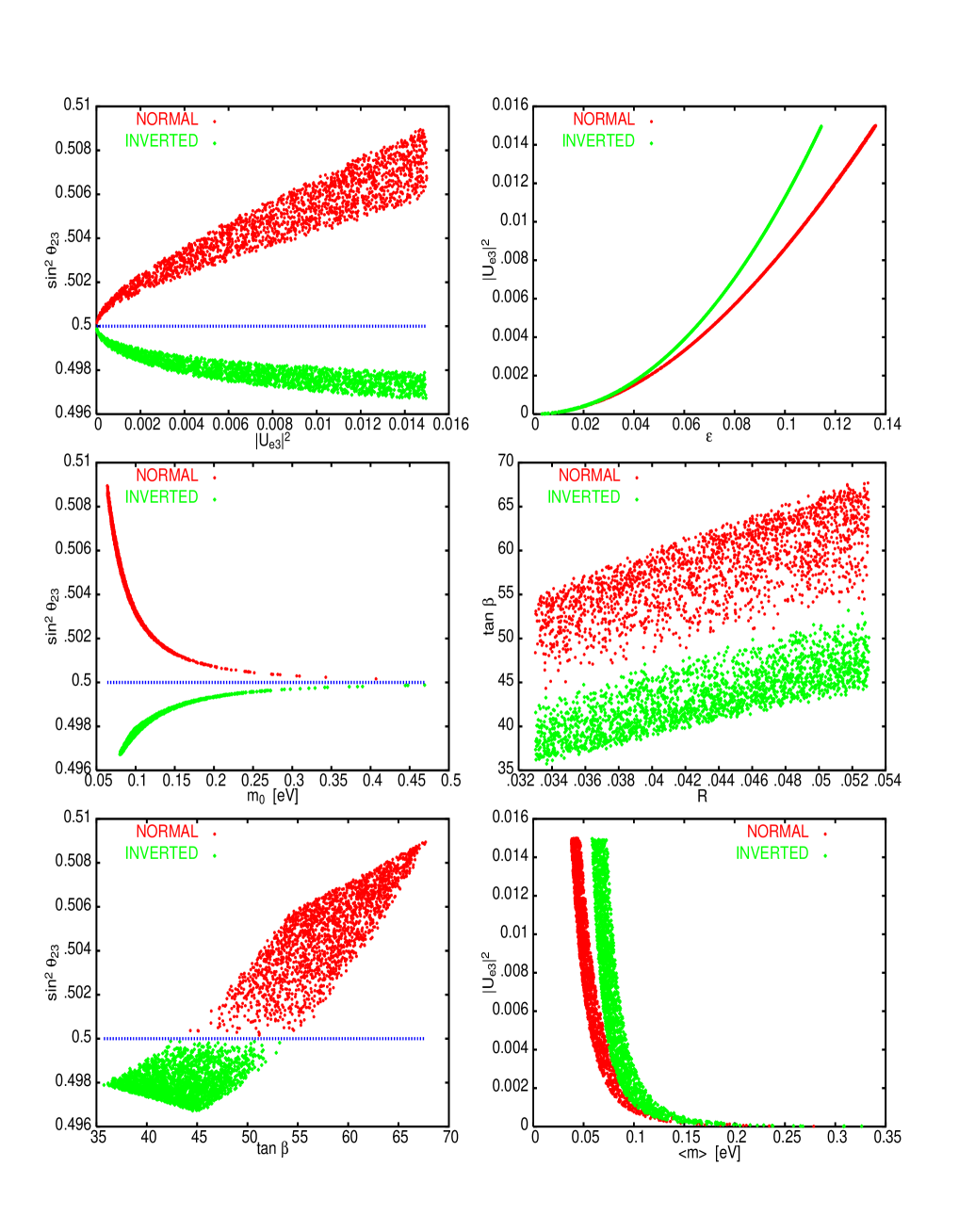
We plot in Fig. 1 some of the resulting correlations of the parameters and observables obtained from an exact numerical analysis, for both the normal and inverted hierarchy. The density of points contains no information, it is rather the envelope of the points which defines the physics. To produce the plots, we demanded the following values for the observables [3, 5, 6, 8]:

$$\tan^{2}\theta_{12} = 0.34\ldots 0.44\;,$$

$$|U_{e3}|^{2} \leq 0.015\;,$$

$$\sin^{2}2\theta_{23} \geq 0.95\;,$$

$$R_{\nu} \equiv \frac{\Delta m^{2}_{\odot}}{\Delta m^{2}_{\rm A}}=0.033\ldots 0.053\;.$$ (27)

Furthermore, since only the ratio of the $\Delta m^{2}$ is required to be correctly reproduced, we restricted the common neutrino mass to be below 0.5 eV. The small parameter $\epsilon$ is bounded from above by $1/\sqrt{10}$. It can be seen from the Figure that,

• the dependence of $U_{e3}$ and $\sin^{2}\theta_{23}$ as given in Eqs. (22,26) is correct. Zero $U_{e3}$ implies $\theta_{23}=\pi/4$ and vice versa;

• $U_{e3}$ and $\sin^{2}\theta_{23}$ follow the functional behavior according to Eqs. (23,24) to a good precision. Hence $U_{e3}\propto 1/m_{0}^{2}$ and $|1/2-\sin^{2}\theta_{23}|\propto 1/m_{0}^{4}$;

• atmospheric neutrino mixing lies on the “dark side” (“light side”) for the normal (inverted) mass ordering;

• the deviation from maximal $\theta_{23}$ can be up to two times larger in case of the normal ordering;

• neutrinoless double beta decay is driven by an effective mass between 0.05 and 0.35 eV (for a given $U_{e3}$ somewhat larger values are expected in case of the inverted ordering) and should therefore be observable (at the latest) in next generation experiments [24];

• the common neutrino mass scale $m_{0}$ is between 0.05 and 0.5 eV and can be probed by next generation cosmological observations [22] and perhaps by the KATRIN laboratory experiment [31];

• for the normal ordering we need $\tan\beta\simeq 35\ldots 50$ and for the inverted ordering $\tan\beta\simeq 45\ldots 65$ is required.

Especially the last issue of the relatively large values of $\tan\beta$ is interesting because many lepton flavor violating processes such as, e.g., $\mu\rightarrow e\gamma$ have a strong dependence on this quantity and can be expected to be sizable. Moreover, an interesting difference with respect to the studies in [19] can be seen. In those works, the matrix Eq. (4) with $c=s$ has been derived from $A_{4}$ symmetry and the most general radiative corrections, including slepton threshold effects, were applied to reproduce the correct neutrino phenomenology. As a result, values of $\tan\beta$ smaller than 8 were required in order to reproduce the observed neutrino phenomenology [19]. Hence, the large difference between the requisite values of $\tan\beta$ may serve as a tool to distinguish the approach in [19] and the one presented here.

We remark that the much discussed [32] claim of a possible evidence of neutrinoless double beta decay, corresponding to $\mbox{$\langle m\rangle$}\simeq 0.1\ldots 0.9$ eV [33], can in principle be accommodated with the flavor symmetry and neutrino mass matrix under study.

We can compare the neutrino oscillation observables obtained in this section with the Ansatz motivated by the near–bimaximal neutrino mixing which led to Eq. (14). For values of $\epsilon\simeq 0.1$ we get $m_{0}\simeq 0.08$ eV from Eq. (19) and $U_{e3}\simeq 0.1$ from Eq. (22). Therefore in the parameterization introduced in [26] and given by Eq. (14), we have $n=1$. The near–maximality of atmospheric neutrino mixing means that $m=3$ and we can compare our results with Eq. (14), when we replace $B$ with $B\lambda^{2}$ in that Equation (note also the relative factor $\sqrt{2}$ for the definition of $m_{0}$ in Eqs. (14) and (15)). Hence, we can estimate $\epsilon\simeq\eta/4\sqrt{2}$ and $\lambda\simeq\epsilon/A$. The result $\epsilon\simeq\eta/4\sqrt{2}$ is also found for the case of very small $\epsilon\mathrel{\hbox to0.0pt{\raise 2.20013pt\hbox{$<$}\hss}{\lower 2.20013pt\hbox{$\sim$}}}0.01$, resulting in small $U_{e3}$ and rather large $m_{0}\mathrel{\hbox to0.0pt{\raise 2.20013pt\hbox{$>$}\hss}{\lower 2.20013pt\hbox{$\sim$}}}0.2$ eV. As a consequence, $\eta\simeq\lambda^{2}\sim\sqrt{8}~{}\epsilon$. Similar arguments apply in the next Subsection, when we allow random order one coefficients for the perturbation to Eq. (4).

A few words on the origin of the democratic perturbation is in order. If $\epsilon$ would come from Planck scale effects [34], then its size would naively be given by $m_{0}~{}\epsilon\simeq v^{2}/M_{\rm Pl}\simeq 2.5\cdot 10^{-6}~{}(m_{0}/{\rm eV})$ eV, with the Planck mass $M_{\rm Pl}\simeq 1.2\cdot 10^{19}$ GeV. Hence, we cannot generate the required values for the neutrino mixing observables. Low scale gravity would effectively replace $M_{\rm Pl}$ with some scale $M_{\tilde{X}}$ in the above considerations. If, say, $M_{\tilde{X}}=10^{16}$ GeV and $m_{0}=0.5$ eV then we could obtain $\Delta m^{2}_{\rm A}$ in the right ballpark. Of course, again values of $\tan\beta\sim 10$ are required to generate a correct $\Delta m^{2}_{\odot}$.

3.2 Anarchical perturbation

In the last Subsection we considered a purely democratic perturbation (see Eq. (15)) to the zeroth order mass matrix conserving $L_{\mu}-L_{\tau}$. In this section we relax this constraint and allow for random order one coefficients for every entry in the perturbation matrix:

$$m_{\nu}=m_{0}\left[\left(\begin{array}[]{ccc}c&0&0\\[8.5359pt] \cdot&0&s\\[8.5359pt] \cdot&\cdot&0\end{array}\right)+\epsilon\left(\begin{array}[]{ccc}a&b&d\\[8.5359pt] \cdot&e&f\\[8.5359pt] \cdot&\cdot&g\end{array}\right)\right]~{},$$ (28)

where $a,b,d,e,f,g$ are real, positive and of order one. Approximate solutions for the oscillation parameters in case of $\theta=3\pi/4$ (i.e., in case of the normal mass ordering) read:

$$U_{e3}\simeq\frac{1}{2}~{}(b+d)~{}\epsilon~{}(1-\epsilon/\sqrt{2})~{}~{}\mbox{ and }\sin^{2}\theta_{23}\simeq\frac{1}{2}+\epsilon~{}\frac{e-g}{\sqrt{8}}~{}.$$ (29)

There is now a term proportional to $\epsilon$ for $\sin^{2}\theta_{23}$, which vanishes for the case of “democracy”, $e=g$. Also, the previous expressions in Eq. (22) are reproduced when $b=d$. The expressions for the $\Delta m^{2}$ are complicated and depend on $\epsilon$ and all six coefficients. In case of the inverted mass ordering, which is again obtained for $\theta\simeq 7\pi/4$, we can estimate

$$U_{e3}\simeq\frac{1}{2}~{}(b+d)~{}\epsilon~{}(1+\epsilon/\sqrt{2})~{}~{}\mbox{ and }~{}~{}\sin^{2}\theta_{23}\simeq\frac{1}{2}-\epsilon~{}\frac{e-g}{\sqrt{8}}~{}.$$ (30)

In contrast to the case treated in Section 3.1, it is no more possible to predict whether atmospheric mixing lies above or below $\pi/4$ because this depends crucially on the relative magnitude of the order one coefficients. Comparing however the expressions for $\sin^{2}\theta_{23}$ in case of normal and inverted mass ordering, we see that for $e>g$ and the normal (inverted) ordering, atmospheric neutrino mixing will be on the “dark side” (“light side”), i.e., $\theta_{23}>(<)\,\pi/4$. For $g>e$ the situation is vice versa. Note further that there are different order one coefficients for $U_{e3}$ and $\sin^{2}\theta_{23}$, making it impossible to write down interesting correlations between the mixing observables. Due to the order one coefficients, we can however expect now broader allowed ranges of $U_{e3}$ and $|\sin^{2}\theta_{23}-1/2|$ than before.

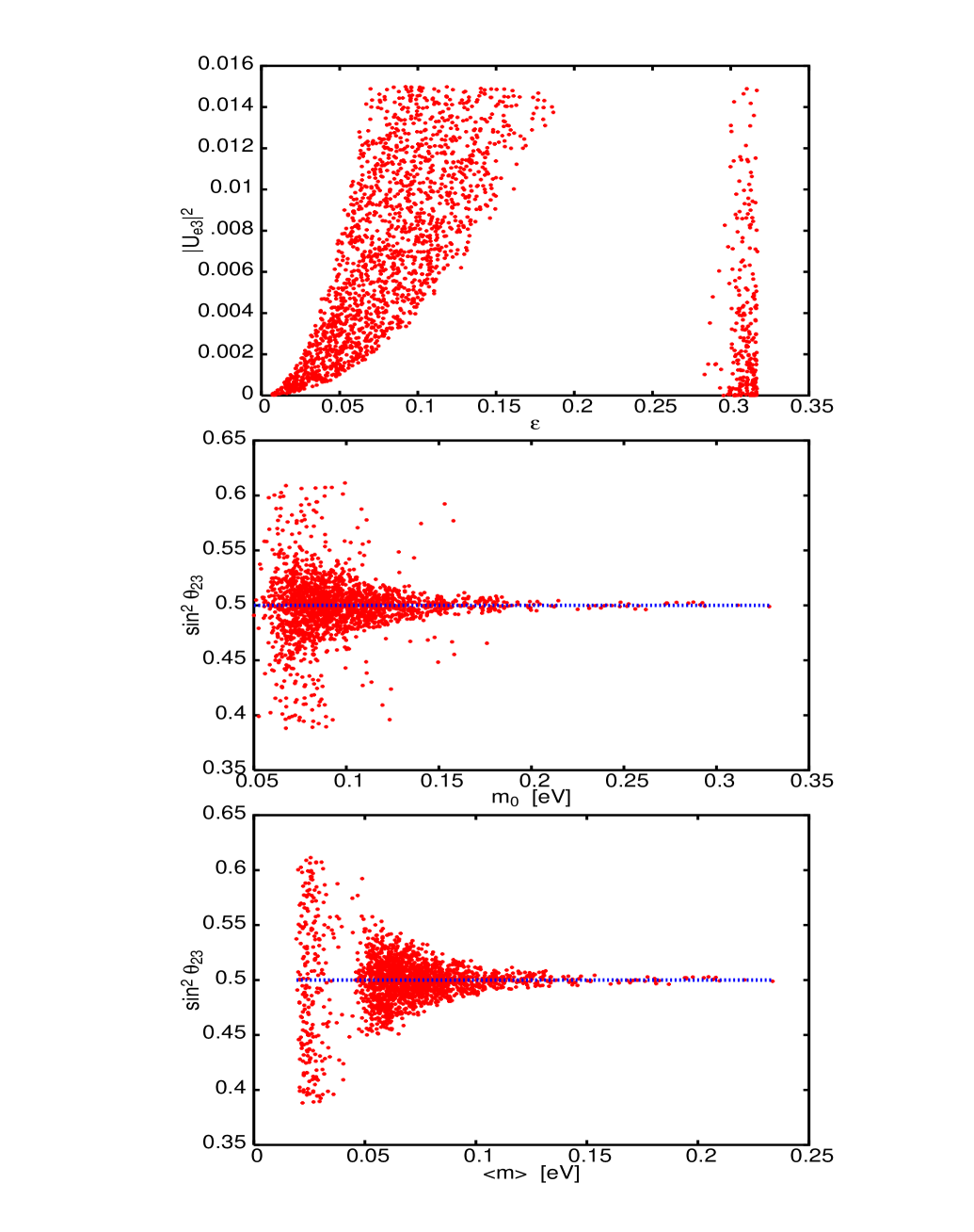
We plot in Fig. 2 some scatter plots of the observables, which are as before required to lie inside the ranges given in Eq. (3.1). All coefficients $a,b,d,e,f,g$ are varied between $1/\sqrt{3}$ and $\sqrt{3}$, $\epsilon$ is again bounded from above by $1/\sqrt{10}$. We find no significant difference between the normal and inverted mass ordering. As excepted, the ranges of the observables are broader than in the case of a purely democratic perturbation. There is also no upper limit on $\epsilon$ any more. Atmospheric neutrino mixing is described by either $\theta_{23}>\pi/4$ or $\theta_{23}<\pi/4$, where the deviation from maximal can be up to 20$\%$. It is also seen that — as in the case of purely democratic perturbation — the larger the neutrino mass scale, the closer $\theta_{23}$ is to $\pi/4$.

4 A Simple Model

In this Section we present a very simple model based on the see–saw [35] mechanism which leads to a low energy mass matrix (approximately) conserving $L^{\prime}\equiv L_{\mu}-L_{\tau}$. The particle content of our model contains only the SM particles plus three heavy Majorana neutrinos $N_{1,2,3}$, which are singlets of the SM gauge group. Under the $U(1)$ symmetry corresponding to $L_{\mu}-L_{\tau}$ the three flavor eigenstates $\nu_{e},\nu_{\mu}$ and $\nu_{\tau}$ have the charges $0,1$ and $-1$, respectively. We can assign now to the usual SM Higgs doublet $\Phi$ the $L^{\prime}$ number 0 and for the three singlets $N_{1},N_{2}$ and $N_{3}$ we choose $L^{\prime}=0,1$ and $-1$, respectively. The relevant Lagrangian is then given by a Dirac mass matrix $m_{D}$ connecting the flavor states and the heavy singlets and by a Majorana mass matrix $M_{R}$ for the latter:

$$\begin{array}[]{c}-{\cal{L}}=\overline{\nu}_{\alpha}\,(m_{D})_{\alpha i}\,N_{i}+\frac{1}{2}N_{i}^{T}C^{-1}\,(M_{R})_{ij}\,N_{j}+h.c.\\[8.5359pt] =\frac{\displaystyle\sqrt{2}}{\displaystyle v}\,\Phi\,\left(a\,\overline{\nu}_{e}N_{1}+b\,\overline{\nu}_{\mu}N_{2}+d\,\overline{\nu}_{\tau}N_{3}\right)+\frac{M}{2}\,\left(X\,N_{1}^{T}C^{-1}N_{1}+Y\,N_{2}^{T}C^{-1}N_{3}\right)+h.c.\end{array}$$ (31)

Here, $a,b,d,X,Y$ are real constants of order one, $M$ is the scale of the heavy singlets, $v/\sqrt{2}$ is the vacuum expectation value of the (lower component) of the Higgs doublet and $C$ is the charge conjugation matrix. With our charge assignment given above, the charged lepton mass matrix is also real and diagonal. After integrating out the heavy singlet states, the neutrino mass matrix $m_{\nu}\simeq-m_{D}^{T}\,M_{R}^{-1}\,m_{D}$ reads

$$m_{\nu}\simeq-\frac{v^{2}}{M}\left(\begin{array}[]{ccc}\displaystyle\frac{a^{2}}{X}&\displaystyle 0&\displaystyle 0\\[8.5359pt] \displaystyle\displaystyle\cdot&\displaystyle 0&\displaystyle\frac{bd}{Y}\\[8.5359pt] \displaystyle\cdot&\displaystyle\cdot&\displaystyle 0\end{array}\right)~{}$$ (32)

and conserves $L_{\mu}-L_{\tau}$. The scale of the neutrino masses $m_{0}=v^{2}/M$ can be adjusted by the in general unknown scale $M$. Note that to explain the global oscillation data one needs $a^{2}/X\simeq bd/Y$, which can for instance be achieved by $a\simeq b\simeq d$ and $X\simeq Y$. A further symmetry is therefore required. As discussed before (cf. with Table 1), this is similar to the case of $L_{e}$ conservation, where the smallness of the determinant of the $\mu\tau$ block is required in order to have large solar neutrino mixing and to the case of $L_{e}-L_{\mu}-L_{\tau}$ where the two entries $m_{e\mu}$ and $m_{e\tau}$ of the mass matrix have to be of the same order for maximal atmospheric neutrino mixing.

We assume now that the heavy Majorana mass matrix softly breaks $L_{\mu}-L_{\tau}$. This can be achieved by adding a democratic perturbation to $M_{R}$. It will then be given by

$$M_{R}=M\left(\begin{array}[]{ccc}X+\epsilon&\epsilon&\epsilon\\[8.5359pt] \cdot&\epsilon&Y+\epsilon\\[8.5359pt] \cdot&\cdot&\epsilon\end{array}\right)~{},$$ (33)

where $\epsilon\ll X,Y$. It is easy to see that for the light neutrino mass matrix the structure of Eq. (28) is reproduced, i.e., an anarchical perturbation is added to Eq. (4). Assuming $a=b=d$ and $X=Y$ will lead to the particularly simple structure of Eq. (15), where a purely democratic perturbation is added to Eq. (4). Of course we can also add a small perturbation to $M_{R}$ which has random order one coefficients. Then the structure given in Eq. (28) will be obtained again.

We note that the model leading to a mass matrix conserving $L_{\mu}-L_{\tau}$ presented in [18] worked with a type II see–saw mechanism [36] and required a larger particle content, namely two Higgs doublets and three triplets. A model similar in spirit to ours has been worked out in [16] for the $L_{e}-L_{\mu}-L_{\tau}$ flavor symmetry, using only two heavy Majorana neutrinos. To successfully reproduce the neutrino oscillation observables, the soft breaking terms in $M_{R}$ had to be of the same order as the $L_{e}-L_{\mu}-L_{\tau}$ conserving terms in [16]. Our model requires only small breaking terms but requires three heavy right–handed neutrinos.

5 Conclusions

The flavor symmetry $L_{\mu}-L_{\tau}$ for the light neutrino mass matrix, on which there are very few analyzes, was considered. It predicts one maximal, two zero mixing angles and quasi–degenerate neutrinos. We showed that demanding the bimaximal mixing scheme and quasi–degenerate neutrinos from the most general neutrino mass matrix yields a matrix obeying this flavor symmetry. Furthermore, a matrix conserving $L_{\mu}-L_{\tau}$ is a special case of $\mu\tau$ symmetric mass matrices. Two simple methods to break $L_{\mu}-L_{\tau}$ were presented. First, we added a purely democratic term to the neutrino mass matrix and applied radiative corrections. Large values of $\tan\beta$ were seen to be required to reproduce the correct neutrino phenomenology. Atmospheric neutrino mixing very close to maximal was predicted. Next, we allowed for random coefficients in the perturbation matrix added to break the $L_{\mu}-L_{\tau}$ symmetry of the the zeroth order mass matrix which strictly conserves $L_{\mu}-L_{\tau}$. Rather large deviations from maximal atmospheric mixing could be generated in this scheme. For the first scheme of $L_{\mu}-L_{\tau}$ symmetry breaking, the observables $U_{e3}^{2}$ and $|1/2-\sin^{2}\theta_{23}|$ were seen to be proportional to the inverse of the fourth power of the common neutrino mass scale, though this interesting behavior was spoiled in the second case due to possible cancellations caused by the different order one parameters. Finally, a simple model based on the see–saw mechanism was presented, which reproduced a neutrino mass matrix conserving $L_{\mu}-L_{\tau}$. Soft and small breaking of the flavor symmetry in the heavy singlet sector was shown to reproduce the two possibilities for symmetry breaking mentioned above.

Acknowledgments

We thank the Scuola Internazionale Superiore di Studi Avanzati, Trieste, where major part of this work was completed. S.C. thanks INFN for financial support during this period. This work was supported by the “Deutsche Forschungsgemeinschaft” in the “Sonderforschungsbereich 375 für Astroteilchenphysik” and under project number RO-2516/3-1 (W.R.).

Figure 1: Scatter plots of some of the correlations of the parameters and observables resulting from Eq. (15) plus applying radiative corrections.

Figure 2: Scatter plots of some of the correlations of the parameters and observables resulting from Eq. (28). The plots are for the inverted mass ordering, the corresponding figure for the normal ordering l ooks basically identical.

References

- [1] B. Pontecorvo, Zh. Eksp. Teor. Fiz. 33, 549 (1957) and 34, 247 (1958); Z. Maki, M. Nakagawa and S. Sakata, Prog. Theor. Phys. 28, 870 (1962).
- [2] M. Apollonio et al. [CHOOZ Collaboration], Eur. Phys. J. C 27, 331 (2003); F. Boehm et al., Phys. Rev. D 64, 112001 (2001).
- [3] E. Kearns, talk given at “Neutrino 2004” June 14-19, 2004, Paris, France, http://neutrino2004.in2p3.fr.
- [4] T. Nakaya et al., talk given at “Neutrino 2004”, June 14-19, 2004, Paris, France, http://neutrino2004.in2p3.fr; M.H. Ahn et al., Phys.Rev.Lett. 90 (2003) 041801; hep-ex/0411038.
- [5] B. T. Cleveland et al., Astrophys. J. 496, 505 (1998); C. Cattadori, Talk at “Neutrino 2004”, Paris, France, June 14-19, 2004 http://neutrino2004.in2p3.fr; S. Fukuda et al. [Super-Kamiokande Collaboration], Phys. Lett. B 539, 179 (2002); S. N. Ahmed et al. [SNO Collaboration], Phys. Rev. Lett. 92, 181301 (2004).
- [6] T. Araki et al., [KamLAND Collaboration], hep-ex/0406035.
- [7] G. L. Fogli et al., hep-ph/0408045.
- [8] See, e.g., A. Bandyopadhyay, et al., hep-ph/0406328; J. N. Bahcall, M. C. Gonzalez-Garcia and C. Pena-Garay, JHEP 0408, 016 (2004).
- [9] M. Maltoni et al., hep-ph/0405172.
- [10] F. Vissani, hep-ph/9708483; V. D. Barger, S. Pakvasa, T. J. Weiler and K. Whisnant, Phys. Lett. B 437, 107 (1998); A. J. Baltz, A. S. Goldhaber and M. Goldhaber, Phys. Rev. Lett. 81, 5730 (1998); H. Georgi and S. L. Glashow, Phys. Rev. D 61, 097301 (2000); I. Stancu and D. V. Ahluwalia, Phys. Lett. B 460, 431 (1999).
- [11] M. Jezabek and Y. Sumino, Phys. Lett. B 457, 139 (1999) Z. z. Xing, Phys. Rev. D 64, 093013 (2001); C. Giunti and M. Tanimoto, Phys. Rev. D 66, 053013 (2002); Phys. Rev. D 66, 113006 (2002); G. Altarelli, F. Feruglio and I. Masina, Nucl. Phys. B 689, 157 (2004); A. Romanino, Phys. Rev. D 70, 013003 (2004); W. Rodejohann, hep-ph/0403236 (to appear in Phys. Rev. D); C. A. de S. Pires, J. Phys. G 30, B29 (2004).
- [12] P. H. Frampton, S. T. Petcov and W. Rodejohann, Nucl. Phys. B 687, 31 (2004).
- [13] S. T. Petcov, W. Rodejohann, hep-ph/0409135.
- [14] F. Vissani, JHEP 9811, 025 (1998).
- [15] S. T. Petcov, Phys. Lett. B 110, 245 (1982); for more recent studies see, e.g., R. Barbieri et al., JHEP 9812, 017 (1998); A. S. Joshipura and S. D. Rindani, Eur. Phys. J. C 14, 85 (2000); R. N. Mohapatra, A. Perez-Lorenzana and C. A. de Sousa Pires, Phys. Lett. B 474, 355 (2000); Q. Shafi and Z. Tavartkiladze, Phys. Lett. B 482, 145 (2000). L. Lavoura, Phys. Rev. D 62, 093011 (2000); W. Grimus and L. Lavoura, Phys. Rev. D 62, 093012 (2000); T. Kitabayashi and M. Yasue, Phys. Rev. D 63, 095002 (2001); A. Aranda, C. D. Carone and P. Meade, Phys. Rev. D 65, 013011 (2002); K. S. Babu and R. N. Mohapatra, Phys. Lett. B 532, 77 (2002); H. J. He, D. A. Dicus and J. N. Ng, Phys. Lett. B 536, 83 (2002) H. S. Goh, R. N. Mohapatra and S. P. Ng, Phys. Lett. B 542, 116 (2002); G. K. Leontaris, J. Rizos and A. Psallidas, Phys. Lett. B 597, 182 (2004).
- [16] L. Lavoura and W. Grimus, JHEP 0009, 007 (2000); hep-ph/0410279.
- [17] P. Binetruy et al., Nucl. Phys. B 496, 3 (1997).
- [18] N. F. Bell and R. R. Volkas, Phys. Rev. D 63, 013006 (2001).
- [19] K. S. Babu, E. Ma and J. W. F. Valle, Phys. Lett. B 552, 207 (2003); M. Hirsch et al., Phys. Rev. D 69, 093006 (2004).
- [20] X. G. He et al., Phys. Rev. D 43, 22 (1991); Phys. Rev. D 44, 2118 (1991); see also E. Ma, D. P. Roy and S. Roy, Phys. Lett. B 525, 101 (2002).
- [21] See e.g., C. S. Lam, Phys. Lett. B 507, 214 (2001); T. Kitabayashi and M. Yasue, Phys. Rev. D 67, 015006 (2003); W. Grimus and L. Lavoura, Phys. Lett. B 572, 189 (2003); E. Ma, Phys. Rev. D 66, 117301 (2002); Y. Koide, Phys. Rev. D 69, 093001 (2004); W. Grimus, et al., hep-ph/0408123; R. N. Mohapatra, JHEP 0410, 027 (2004).
- [22] S. Hannestad, JCAP 0305, 004 (2003); hep-ph/0409108.
- [23] U. Seljak et al., astro-ph/0407372.
- [24] See, e.g., S. R. Elliott and J. Engel, J. Phys. G 30, R183 (2004) and references therein.
- [25] W. Rodejohann, Nucl. Phys. B 597, 110 (2001); Z. z. Xing, Phys. Rev. D 68, 053002 (2003); more realistic recent analyzes are V. Barger et al., Phys. Lett. B 540, 247 (2002); S. Pascoli, S. T. Petcov and W. Rodejohann, Phys. Lett. B 549, 177 (2002); F. Deppisch, H. Pas and J. Suhonen; hep-ph/0409306; A. Joniec, M. Zralek, hep-ph/0411070.
- [26] W. Rodejohann, Phys. Rev. D 69, 033005 (2004).
- [27] M. Raidal, Phys. Rev. Lett. 93, 161801 (2004); H. Minakata and A. Y. Smirnov, hep-ph/0405088; P. H. Frampton and R. N. Mohapatra, hep-ph/0407139; see also J. Ferrandis and S. Pakvasa, hep-ph/0409204.
- [28] See, e.g., J.A. Casas, et al., Nucl. Phys. B 573, 652 (2000); P.H. Chankowski, S. Pokorski, Int. J. Mod. Phys. A 17 (2002) 575; S. Antusch, et al., Nucl. Phys. B 674, 401 (2003).
- [29] S. Antusch et al., hep-ph/0404268; H. Minakata, M. Sonoyama and H. Sugiyama, hep-ph/0406073; M. C. Gonzalez-Garcia, M. Maltoni and A. Y. Smirnov, hep-ph/0408170; S. Choubey and P. Roy, Phys. Rev. Lett. 93, 021803 (2004).
- [30] J. Bernabeu, S. Palomares Ruiz and S. T. Petcov, Nucl. Phys. B 669, 255 (2003); O. L. G. Peres and A. Y. Smirnov, Nucl. Phys. B 680, 479 (2004); S. Palomares-Ruiz and S. T. Petcov, hep-ph/0406096.
- [31] A. Osipowicz et al. [KATRIN Collaboration], hep-ex/0109033.
- [32] H. V. Klapdor-Kleingrothaus et al., Mod. Phys. Lett. A 16, 2409 (2001); C. E. Aalseth et al., Mod. Phys. Lett. A 17, 1475 (2002); H. L. Harney, hep-ph/0205293; H. V. Klapdor-Kleingrothaus, hep-ph/0205228; F. Feruglio, A. Strumia and F. Vissani, Nucl. Phys. B 637, 345 (2002) [Addendum-ibid. B 659, 359 (2003)].
- [33] H. V. Klapdor-Kleingrothaus et al., Phys. Lett. B 586, 198 (2004).
- [34] E. K. Akhmedov, Z. G. Berezhiani and G. Senjanovic, Phys. Rev. Lett. 69, 3013 (1992); E. K. Akhmedov et al., Phys. Rev. D 47, 3245 (1993); A. de Gouvea and J. W. F. Valle, Phys. Lett. B 501, 115 (2001); F. Vissani, M. Narayan and V. Berezinsky, Phys. Lett. B 571, 209 (2003); hep-ph/0401029.
- [35] P. Minkowski, Phys. Lett. B67, 421 (1977); T. Yanagida, in Proceedings of the Workshop on Unified Theory and the Baryon Number of the Universe, edited by O. Sawada and A. Sugamoto (KEK, Tsukuba, 1979), p. 95; M. Gell-Mann, P. Ramond, and R. Slansky, in Supergravity, edited by F. van Nieuwenhuizen and D. Freedman (North Holland, Amsterdam, 1979), p. 315; S.L. Glashow, in Quarks and Leptons, edited by M. L et al. (Plenum, New York, 1980), p. 707; R.N. Mohapatra and G. Senjanovic, Phys. Rev. Lett. 44, 912 (1980).
- [36] J. Schechter and J.W.F. Valle, Phys. Rev. D 22, 2227 (1980); M. Magg and C. Wetterich, Phys. Lett. B 94, 61 (1980); R. N. Mohapatra and G. Senjanovic, Phys. Rev. D 23, 165 (1981); G. Lazarides, Q. Shafi and C. Wetterich, Nucl. Phys. B 181, 287 (1981).