Rare top quark decay $t\to u_{1}\bar{u}_{2}u_{2}$ in the standard model

Abstract

The one-loop induced top quark decay $t\to u_{1}\bar{u}_{2}u_{2}$ ($u_{i}=u,c$) is calculated in the context of the standard model. The dominant contribution to this top quark decay arises from the Feynman diagrams induced by the off-shell $tu_{1}g^{*}$ vertex, whereas the box diagrams are negligibly small. In contrast with the on-shell $tu_{1}g$ vertex, which only gives rise to a pure dipolar effect, the off-shell $tu_{1}g^{*}$ coupling also involves a monopolar term, which gives a larger contribution than the dipolar one. It is found that the branching ratio for the three-body decay $t\to u_{1}\bar{u}_{2}u_{2}$ is about of the same order of magnitude of the two-body decay $t\to u_{1}g$, which stems from the fact that the three-body decay is dominated by the monopolar term.

I Introduction

The top quark detection at the Fermilab Tevatron CDF greatly boosted the interest in top quark physics. The large mass of this quark suggests that it could be very sensitive to new physics effects, which may manifest themselves through anomalous rates for its production and decay modes. Although some properties of the top quark have already been examined at the Tevatron PTevatron , a further scrutiny is expected at the CERN large hadron collider (LHC). This machine will operate as a veritable top quark factory, producing about eight millions of $\bar{t}t$ events per year in its first stage, and hopefully up to about eighteen millions in subsequent years TOPReviews . Yet in the first stage of the LHC, many rare processes involving the top quark are expected to be accessible. It is thus worth investigating all of the top quark decays within the standard model (SM) in order to find out any scenario that may be highly sensitive to new physics effects.

In the SM, the main decay channel of the top quark is $t\to bW$. Although the nondiagonal $t\to dW$ and $t\to sW$ modes are more suppressed, they still have sizable branching ratios. For instance, $Br(t\to sW)$ is of the order of $10^{-3}$. As far as rare decays are concerned, the three-body tree-level induced modes $t\to d_{i}WZ$ and $t\to u_{1}WW$, with $d_{i}=b,s,d$ and $u_{1}=u,c$, are strongly dependent on the precise value of the top quark mass. It has been shown that the $t\to u_{1}WW$ decays are severely GIM-suppressed Jenkins , but $t\to bWZ$ can have a branching ratio of the order of $10^{-5}$ for a top quark mass larger than $187$ GeV Decker . This decay mode has been suggested as a probe for the top quark mass because it is almost in the threshold region PDG . At the one-loop level, there arise the flavor changing neutral current (FCNC) decays $t\to u_{1}V$ ($V=g,\,\gamma\,Z$) and $t\to u_{1}H$, which are considerably GIM-suppressed, with branching ratios ranging from $10^{-10}$ to $10^{-13}$ Eilam ; Diaz ; Mele . Motivated by the fact that any process that is forbidden or strongly suppressed within the SM constitutes a natural laboratory to search for any new physics effects, FCNC top quark decays have been the subject of considerable interest in the literature THDM ; SUSY ; SUSYR ; EXOTIC ; EFT . It turns out that they may have large branching ratios, much larger than the SM ones, within some extended theories such as the two-Higgs doublet model (THDM) THDM , supersymmetry (SUSY) models with nonuniversal soft breaking SUSY , SUSY models with broken $R$-parity SUSYR , and even more exotic scenarios EXOTIC . Similar results for the decays $t\to u_{1}V$ and $t\to u_{1}H$ were obtained within the context of effective theories EFT .

In this work, we present a calculation of the $t\to u_{1}\bar{u}_{2}u_{2}$ decay ($u_{2}$ stands for the $u$ or $c$ quark), which arises at the one-loop level in the SM. Although the study of rare top quark transitions has attracted considerable attention, to our knowledge the rare decay $t\to u_{1}\bar{u}_{2}u_{2}$ has never been analyzed before. The rest of the paper is organized as follows. Section II is devoted to the analytical calculation of the decay $t\to u_{1}\bar{u}_{2}u_{2}$. The numerical results and discussion are presented in Sec. III along with the final remarks.

II The decay $t\to u_{1}\bar{u}_{2}u_{2}$

Decays of the type $t\to u_{1}\bar{u}_{2}u_{2}$ proceed through the reducible diagrams shown in Fig. 1$(i)$, which are mediated by the $Z$, $H$, $\gamma$ or $g$ bosons. While those Feynman diagrams mediated by the $Z$ and $H$ bosons are enhanced due to the fact that the intermediary boson is on resonance (provided that $m_{H}\leq m_{t}$), those diagrams mediated by the photon (gluon) are enhanced by the effect of the photon (gluon) pole. There are also contributions from box diagrams carrying $W$ gauge bosons and down quarks [see Fig. 1$(ii)$]. Since each type of diagram renders a finite amplitude by its own, the different contributions can be considered as independent. It can be shown that the $t\to u_{1}\bar{u}_{2}u_{2}$ decay is essentially determined by those graphs involving a virtual gluon, i.e., those reducible diagrams involving the one-loop vertex $tu_{1}g^{*}$ and the tree-level vertex $g^{*}\bar{u}_{2}u_{2}$. The role played by this contribution is evident from the fact that it constitutes an electroweak-QCD mixed effect. This is to be contrasted with those reducible graphs mediated by the $\gamma$, $Z$ and $H$ bosons, as well as the box diagrams, which are entirely determined by electroweak couplings. As a consequence, the pure electroweak contributions become suppressed by a factor of $\alpha/\alpha_{s}$ as compared with the electroweak-QCD mixed ones.

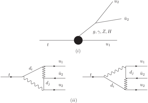
Figure 1: Feynman diagrams contributing to the $t\to u_{1}u_{2}\bar{u}_{2}$ decay. The bubble stands for all the contributions of the type shown in Fig. 2.

Once the most relevant properties of the $t\to u_{1}\bar{u}_{2}u_{2}$ decay were described, we would like to emphasize a noteworthy feature of this process. It is closely related to the fact that the $t\to u_{1}\bar{u}_{2}u_{2}$ decay is mediated by a virtual massless vector boson, i.e., the gluon or the photon. Without losing generality, it is enough to discuss the gluon contribution as it is the dominant one. Naively, one would expect that the rate for the two-body decay $t\to u_{1}g$ is larger than that for the three-body decay $t\to u_{1}\bar{u}_{2}u_{2}$, which in fact is not true. This stems from the fact that while the on-shell $tu_{1}g$ vertex is characterized by a dipole structure (the $tu_{1}$ pair couples to the gluon through the gauge tensor $G^{a}_{\mu\nu}$), the corresponding off-shell $tu_{1}g^{*}$ vertex involves also a monopole structure (the $tu_{1}$ pair interacts directly with the $A^{a}_{\mu}$ gauge field). Therefore, while the $t\to u_{1}g$ transition is entirely determined by the dipole structure, both the dipole and the monopole structures contribute to the $t\to u_{1}\bar{u}_{2}u_{2}$ process. It turns out that the contribution from the monopolar term can be considerably larger than that arising from the dipolar one. We have found that this is indeed the case for the rare decay $t\to u_{1}\bar{u}_{2}u_{2}$. It means that while the $t\to u_{1}g$ decay is determined by the dipolar term, the $t\to u_{1}\bar{u}_{2}u_{2}$ mode is governed by the monopolar one. Moreover, the three-body decay is unsuppressed because it includes the QCD vertex $g^{*}\bar{u}_{2}u_{2}$, which is much less suppressed than the electroweak vertices $\gamma^{*}\bar{u}_{2}u_{2}$ and $Z^{*}\bar{u}_{2}u_{2}$. The above properties nicely conspire to enhance the $t\to u_{1}\bar{u}_{2}u_{2}$ decay rate by about one order of magnitude with respect to that of the $t\to u_{1}g$ transition.

Figure 2: Feynman diagrams contributing to the $tu_{1}g$ vertex in the unitary gauge. In the $R_{\xi}$ gauge there are an extra set of diagrams in which the $W$ boson is replaced by its associate pseudogoldstone boson.

We now turn to analyze the general structure of the $tu_{1}g$ vertex, which is generated at the one-loop level via the Feynman diagrams shown in Fig. 2. The most general form of this vertex involves up to ten form factors, which are associated with the Lorentz structures $\gamma_{\mu}P_{L,R}$, $(p-p_{1})_{\mu}P_{L,R}$, $q_{\mu}P_{L,R}$, $\sigma_{\mu\nu}(p-p_{1})^{\nu}P_{L,R}$, and $\sigma_{\mu\nu}q^{\nu}P_{L,R}$, with $P_{L,R}=(1\mp\gamma_{5})/2$. There are however a few independent form factors. After imposing the on-shell conditions on the fermionic fields, the Gordon identities allows one to eliminate the four form factors associated with $(p-p_{1})_{\mu}P_{L,R}$ and $\sigma_{\mu\nu}(p-p_{1})^{\nu}P_{L,R}$. In addition, the $q_{\mu}\epsilon^{\mu}=0$ condition, valid for a real gluon, can be safely used as the off-shell gluon couples to a pair of approximately massless quarks. Thus, the only non negligible contributions to the the $t\to u_{1}\bar{u}_{2}u_{2}$ decay are those of the monopolar ($\gamma_{\mu}P_{L,R}$) and dipolar ($\sigma_{\mu\nu}q^{\nu}P_{L,R}$) terms. Furthermore, no contributions proportional to $P_{R}$ can arise in the $m_{u_{1}}=0$ limit. Consequently, the vertex function associated with the $tu_{1}g$ coupling can be written as

$$\Gamma^{a}_{\mu}=\frac{\lambda^{a}}{2}\Gamma_{\mu}=\left(\frac{\lambda^{a}}{2}\right)ig_{s}\left[F_{1}(q^{2})\gamma_{\mu}P_{L}+\frac{i}{m_{t}}F_{2}(q^{2})P_{L}\sigma_{\mu\nu}q^{\nu}\right],$$ (1)

where $g_{s}$ is the coupling constant and $\lambda^{a}/2$ stand for the generators associated with the color group. It is worth mentioning that the monopolar contribution $F_{1}$ vanishes in the on-shell limit as a consequence of the Ward identity $q^{\mu}\Gamma_{\mu}=0$. This means that a FCNC vertex involving an on-shell gluon can only arise through a dipolar term, such as occurs in electrodynamics. This is not true for an off-shell gluon: in such a case the monopolar term yields the dominant contribution. This behavior will be explicitly shown below. We will first calculate the form factors in an $R_{\xi}$ gauge and, in order to assure that our result is gauge-independent, we will also calculate such form factors via the unitary gauge. In the $R_{\xi}$ gauge the calculation leads to the following amplitude

$$\Gamma_{\mu}=\frac{g_{s}g^{2}}{2}\sum_{i}V_{u_{1}i}V^{\dagger}_{it}\int\frac{d^{D}k}{(2\pi)^{D}}\sum^{6}_{a=1}\frac{T^{a}_{\mu}}{\Delta_{a}},$$ (2)

where

$$T^{1}_{\mu}=\gamma_{\beta}P_{L}(\hbox{\large$/$}\kern-5.76042pt\hbox{$k$}+\hbox{\large$/$}\kern-6.91562pt\hbox{$p_{2}$}+m_{i})\gamma_{\mu}(\hbox{\large$/$}\kern-5.76042pt\hbox{$k$}+\hbox{\large$/$}\kern-6.91562pt\hbox{$p_{1}$}+m_{i})\gamma_{\alpha}P_{L}P^{\alpha\beta},$$ (3)

$$T^{2}_{\mu}=-\left(\frac{1}{m^{2}_{t}}\right)\gamma_{\beta}P_{L}(\hbox{\large$/$}\kern-5.76042pt\hbox{$k$}+\hbox{\large$/$}\kern-6.91562pt\hbox{$p_{2}$}+m_{i})\gamma_{\alpha}P_{L}(\hbox{\large$/$}\kern-6.91562pt\hbox{$p_{2}$}+m_{t})\gamma_{\mu}P^{\alpha\beta},$$ (4)

$$T^{3}_{\mu}=\left(\frac{1}{m^{2}_{t}}\right)\gamma_{\mu}\hbox{\large$/$}\kern-6.91562pt\hbox{$p_{1}$}\gamma_{\beta}P_{L}(\hbox{\large$/$}\kern-5.76042pt\hbox{$k$}+\hbox{\large$/$}\kern-6.91562pt\hbox{$p_{1}$}+m_{i})\gamma_{\alpha}P_{L}P^{\alpha\beta},$$ (5)

$$T^{4}_{\mu}=\Big{(}\frac{m_{i}}{m^{2}_{W}}\Big{)}P_{R}(\hbox{\large$/$}\kern-5.76042pt\hbox{$k$}+\hbox{\large$/$}\kern-6.91562pt\hbox{$p_{2}$}+m_{i})\gamma_{\mu}(\hbox{\large$/$}\kern-5.76042pt\hbox{$k$}+\hbox{\large$/$}\kern-6.91562pt\hbox{$p_{1}$}+m_{i})(m_{t}P_{R}-m_{i}P_{L}),$$ (6)

$$T^{5}_{\mu}=-\Big{(}\frac{1}{m^{2}_{t}}\Big{)}\Big{(}\frac{m_{i}}{m^{2}_{W}}\Big{)}P_{R}(\hbox{\large$/$}\kern-5.76042pt\hbox{$k$}+\hbox{\large$/$}\kern-6.91562pt\hbox{$p_{2}$}+m_{i})(m_{t}P_{R}-m_{i}P_{L})(\hbox{\large$/$}\kern-6.91562pt\hbox{$p_{2}$}+m_{t})\gamma_{\mu},$$ (7)

$$T^{6}_{\mu}=\Big{(}\frac{1}{m^{2}_{t}}\Big{)}\Big{(}\frac{m_{i}}{m^{2}_{W}}\Big{)}\gamma_{\mu}\hbox{\large$/$}\kern-6.91562pt\hbox{$p_{1}$}(\hbox{\large$/$}\kern-5.76042pt\hbox{$k$}+\hbox{\large$/$}\kern-6.91562pt\hbox{$p_{1}$}+m_{i})(m_{t}P_{R}-m_{i}P_{L}),$$ (8)

$$\Delta_{1}=[k^{2}-m^{2}_{W}][(k+p_{1})^{2}-m^{2}_{i}][(k+p_{2})^{2}-m^{2}_{i}],$$ (9)

$$\Delta_{2}=[k^{2}-m^{2}_{W}][(k+p_{2})^{2}-m^{2}_{i}],$$ (10)

$$\Delta_{3}=[k^{2}-m^{2}_{W}][(k+p_{1})^{2}-m^{2}_{i}],$$ (11)

$$\Delta_{4}=[k^{2}-\xi m^{2}_{W}][(k+p_{1})^{2}-m^{2}_{i}][(k+p_{2})^{2}-m^{2}_{i}],$$ (12)

$$\Delta_{5}=[k^{2}-\xi m^{2}_{W}][(k+p_{2})^{2}-m^{2}_{i}],$$ (13)

$$\Delta_{6}=[k^{2}-\xi m^{2}_{W}][(k+p_{1})^{2}-m^{2}_{i}],$$ (14)

and

$$P^{\alpha\beta}=g^{\alpha\beta}-\frac{(1-\xi)k^{\alpha}k^{\beta}}{k^{2}-\xi m^{2}_{W}}.$$ (15)

In the previous expressions, the $m_{u_{1}}=0$ approximation was used. In addition, $m_{i}$ denotes the mass of the internal down quark and $\xi$ is the gauge parameter. For simplicity the calculation was performed in the t’Hooft-Feynman gauge ($\xi=1$). As a crosscheck, we also have performed the calculation via the unitary gauge($\xi=\infty$), in which there are only contributions from the first three terms in Eq. (2), with $P^{\alpha\beta}$ replaced by $P^{\alpha\beta}=g^{\alpha\beta}-k^{\alpha}k^{\beta}/m^{2}_{W}$. The results obtained by these two calculation schemes do coincide, which guarantees that the form factors associated with the monopolar and dipolar structures of the $tu_{1}g^{*}$ vertex are gauge-independent. Introducing the definition $F_{i}=(\alpha^{2}/8\pi)A_{i}$ we can write

$$A_{1} = \frac{x}{2x_{W}(1-x)}\sum_{i=d,s,b}V_{u_{1}i}V_{ti}^{\dagger}\left(f^{1}_{0}+\sum^{3}_{a=1}f^{1}_{a}B_{0}(a)+2m^{2}_{t}\,g_{1}\,C_{0}(x,x_{i})\right),$$ (16)

$$A_{2} = \frac{1}{2x_{W}(1-x)}\sum_{i=d,s,b}V_{u_{1}i}V_{ti}^{\dagger}\left(f^{2}_{0}+\sum^{3}_{a=1}f^{2}_{a}B_{0}(a)+2m^{2}_{t}\,g_{2}\,C_{0}(x,x_{i})\right),$$ (17)

where $x=q^{2}/m^{2}_{t}$, $x_{W}=m^{2}_{W}/m^{2}_{t}$, and $x_{i}=m^{2}_{i}/m^{2}_{t}$. The $f^{b}_{a}$ functions depend on $x_{i}$ and read

$$f^{1}_{0}=x_{i},$$ (18)

$$f^{1}_{1} = \frac{1}{1-x}\Bigg{(}\Big{(}2(1-x)+(x-4)(x_{i}+x_{W})\Big{)}x_{i}$$ (19)

$$- 2\Big{(}2(1-x)+(x-4)x_{W}\Big{)}x_{W}\Bigg{)},$$

$$f^{1}_{2} = \frac{1}{(1-x)^{2}}\Bigg{(}(x+2)\Big{(}1-x-2(x_{i}+x_{W})\Big{)}x_{i}$$ (20)

$$+ 2\Big{(}2(x+2)x_{W}-x(1-x)-2(1-x^{2})\Big{)}x_{W}\Bigg{)}$$

$$f^{1}_{3} = \frac{1}{(1-x)^{2}}\Bigg{(}\Big{(}-x^{2}+5x-4+(x^{2}-3x+8)(x_{i}+x_{W})\Big{)}x_{i}$$ (21)

$$- 2\Big{(}x^{2}+3x-4+(x^{2}-3x+8)x_{W}\Big{)}x_{W}\Bigg{)},$$

$$g_{1} = \frac{1}{(1-x)^{2}}\Bigg{(}2\Big{(}x(1-x)^{2}+(x+2)x^{2}_{W}+2(x^{2}-1)x_{W}\Big{)}x_{W}$$ (22)

$$+ \Big{(}(1-x)^{2}(x_{i}-1)+(x+2)(x^{2}_{i}-3x^{2}_{W})-2((x+1)^{2}-4)x_{W}\Big{)}x_{i}\Bigg{)},$$

and

$$f^{2}_{0}=x_{i},$$ (23)

$$f^{2}_{1} = \frac{1}{1-x}\Bigg{(}\Big{(}2(1-x)-(x+2)(x_{i}+x_{W})\Big{)}x_{i}$$ (24)

$$- 2\Big{(}2(1-x)-(x+2)x_{W}\Big{)}x_{W}\Bigg{)},$$

$$f^{2}_{2} = \frac{x}{(1-x)^{2}}\Bigg{(}3\Big{(}1-x-2(x_{i}+x_{W})\Big{)}x_{i}$$ (25)

$$+ 2\Big{(}6x_{W}-5(1-x)\Big{)}x_{W}\Bigg{)},$$

$$f^{2}_{3} = \frac{1}{(1-x)^{2}}\Bigg{(}\Big{(}x^{2}+x-2-(x^{2}-5x-2)(x_{i}+x_{W})\Big{)}x_{i}$$ (26)

$$- 2\Big{(}3x^{2}-x-2-(x^{2}-5x-2)x_{W}\Big{)}x_{W}\Bigg{)},$$

$$g_{2} = \frac{1}{(1-x)^{2}}\Bigg{(}2x\Big{(}(1-x)(1-x-4x_{W})+3x^{2}_{W}\Big{)}x_{W}$$ (27)

$$+ \Big{(}3xx^{2}_{i}+(x_{i}-1)(1-x)^{2}+(2(1+2x)-3x(2x+3x_{W}))x_{W}\Big{)}x_{i}\Bigg{)},$$

In writing the above expressions, the unitarity condition $\sum_{i}V_{u_{1}i}V^{\dagger}_{ti}=0$ was taken into account, i.e., any term independent of the internal quark mass was dropped out. Also, it is straightforward to show that $\sum^{3}_{a=1}f^{b}_{a}=0$ for $b=1,\,2$, which means that, as expected, the $A_{i}$ amplitudes are free of ultraviolet divergences.

We now are ready to calculate the contribution of the $tu_{1}g^{*}$ vertex to the $t\to u_{1}\bar{u}_{2}u_{2}$ decay. Below, $p_{2}$ and $\bar{p}_{2}$ will stand for the 4-momenta associated with the $u_{2}$ and $\bar{u}_{2}$ quarks. It is useful to introduce the following dimensionless variable $y=(p_{1}+\bar{p}_{2})^{2}/m^{2}_{t}$. The $u_{1}$ quark mass will be retained in the phase space integral since a factor of $1/x^{2}$, associated with the gluon pole, enters into the $t\to u_{1}\bar{u}_{2}u_{2}$ squared amplitude. Using the expressions for the $tu_{1}g^{*}$ and $g^{*}u_{2}u_{2}$ vertices, it is straightforward to construct the invariant amplitude associated with the diagram $(i)$ of Fig. 1. After making this, we can write the invariant mass distribution $d\Gamma/dx$ as follows

$$\frac{d\Gamma(t\to u_{1}u_{2}\bar{u}_{2})}{dx}=\frac{m_{t}}{256\pi^{3}}\int dy\sum_{spins}|\mathcal{M}|^{2},$$ (28)

with the squared amplitude being

$$\sum_{spins}|\mathcal{M}|^{2} = \frac{\alpha^{2}_{s}\alpha^{2}}{9s_{W}^{4}\,x^{2}}\left(F_{1}(x,y)|A_{1}|^{2}+F_{12}(x,y)2Re(A_{1}A^{*}_{2})\right.$$ (29)

$$+ \left.F_{2}(x,y)|A_{2}|^{2}\right),$$

As far as the $F_{i}(x,y)$ functions are concerned, they are given by

$$F_{1}(x,y)=-4\Big{(}x^{2}+x(2y-1)+2y(y-1)\Big{)},$$ (30)

$$F_{12}(x,y)=-4x(1-x),$$ (31)

$$F_{2}(x,y)=4x\Big{(}2y(y-1)+x(2y-1)+1\Big{)}.$$ (32)

whereas the Passarino-Veltman scalar functions $B_{0}$ and $C_{0}$ are, in the usual notation:

$$B_{0}(1)=B_{0}(0,m_{t}^{2}x_{i},m^{2}_{W}),$$ (33)

$$B_{0}(2)=B_{0}(m^{2}_{t}x,m_{t}^{2}x_{i},m_{t}^{2}x_{i}),$$ (34)

$$B_{0}(3)=B_{0}(m^{2}_{t},m_{t}^{2}x_{i},m^{2}_{W}),$$ (35)

$$C_{0}(x,x_{i})=C_{0}(m^{2}_{t},0,m^{2}_{t}x,m_{t}^{2}x_{i},m^{2}_{W},m_{t}^{2}x_{i}).$$ (36)

The integration limits are as follows

$$y_{min} = y_{0}^{2}+\frac{1}{2}(1-x)\left(1-\sqrt{1-\frac{4y^{2}_{0}}{x}}\right),$$ (37)

$$y_{max} = y_{0}^{2}+\frac{1}{2}(1-x)\left(1+\sqrt{1-\frac{4y^{2}_{0}}{x}}\right),$$ (38)

$$4y^{2}_{0}\leq x\leq(1-x_{0})^{2},$$ (39)

where $x_{0}=m_{u_{1}}/m_{t}$ and $y_{0}=m_{u_{2}}/m_{t}$.

From Eq. (16) it is evident that $A_{1}$, the monopole term, vanishes in the on-shell limit ($x\to 0$), in agreement with the fact that the $t\to u_{1}g$ decay is only determined by a dipole term. We will show below that the monopole contribution is slightly larger than the dipole one.

Since the $A_{i}$ amplitudes do not depend on $y$, this variable can be integrated over readily. In the $y_{0}\to 0$ limit, we are left with

$$\frac{d\Gamma}{dx}=\frac{\alpha^{2}_{s}\alpha^{2}m_{t}}{1728\,s_{W}^{4}\,\pi^{3}}\left(f_{1}(x)|A_{1}|^{2}+f_{12}(x)Re(A_{1}A^{*}_{2})+f_{2}(x)|A_{2}|^{2}\right),$$ (40)

where

$$f_{1}(x) = \frac{1}{x^{2}}(1+2x)(1-x)^{2},$$ (41)

$$f_{12} = -\frac{6}{x}(1-x)^{2},$$ (42)

$$f_{2}(x) = \frac{1}{x}(2+x)(1-x)^{2}.$$ (43)

It is interesting to note that we will not take into account the limiting case $y_{0}\to 0$ ($m_{u_{2}}=0$) when integrating over $x$ because the $d\Gamma/dx$ distribution would become undefined in $x=0$ due to the gluon pole. This corresponds to the case when the $u_{2}$ quark emerges parallel to $\bar{u}_{2}$ and we cannot take the limit of massless $u_{2}$ quark as it would lead to a collinear singularity. Thus, although we have neglected the outgoing quark masses in the transition amplitude, they must be retained in the integration limits of the $x$ variable.

III Numerical Results and Final remarks

For the numerical analysis we will use the values of the running coupling constant $\alpha_{s}$ and quark masses at the $m_{t}$ scale, namely, $\alpha_{s}(m_{t})=0.10683$, $m_{t}(m_{t})=174.3$ GeV, $m_{b}(m_{t})=2.85$ GeV, $m_{c}(m_{t})=0.63$ GeV, $m_{s}(m_{t})=0.09$ GeV, $m_{d}(m_{t})=0.0049$ GeV, and $m_{u}(m_{t})=0.00223$ GeV Fusaoka . It is worth noting that the numerical results do not change considerably for small variations of the outgoing quark masses.

We first would like to compare the size of the off-shell $tu_{1}g^{*}$ vertex with that of the on-shell one. Numerical evaluation shows that the $tu_{1}g$ dipole contribution is two orders of magnitude smaller than the $tu_{1}g^{*}$ monopole contribution and one order smaller than the $tu_{1}g^{*}$ dipole contribution. Thus, while the $t\to u_{1}g$ decay only receives the contribution of the dipolar term, the $t\to u_{1}\bar{u}_{2}u_{2}$ transition receives an extra contribution of the monopolar term, which is slightly larger than the dipolar contribution.

The fact that the contribution of the monopole form factor to the $tu_{1}g^{*}$ vertex is larger than that of the dipole one is exhibited in the invariant mass distribution $d\Gamma(t\to u_{1}\bar{u}_{2}u_{2})/dx$, which is shown in Fig. 3, where we have plotted separately the monopolar and dipolar contributions. Therefore, it is evident that the $t\to u_{1}\bar{u}_{2}u_{2}$ decay is slightly dominated by the monopolar term.

Figure 3: Monopolar and dipolar contributions to the $t\to u_{1}\bar{u}_{2}u_{2}$ invariant mass distribution $d\Gamma/dx$.

We now turn to the numerical evaluation of $Br(t\to u_{1}\bar{u}_{2}u_{2})$. Using the values given above and $\Gamma(t\to bW)=1.55$ GeV, we obtain

$$Br(t\to u_{1}\bar{u}_{2}u_{2})=3.38\times 10^{-12}.$$ (44)

On the other hand, according to the literature $Br(t\to u_{1}g)=5.73\times 10^{-12}$ Eilam ; Eilam2 . This result shows that $Br(t\to u_{1}\bar{u}_{2}u_{2})$ is about of the same order of magnitude than $Br(t\to u_{1}g)$. If one sums over all the possible $\bar{u}_{2}u_{2}$ pairs, the resulting $Br(t\to u_{1}\bar{u}_{2}u_{2})$ is of the order of $10^{-11}$ and thus larger than $BR(t\to u_{1}g)$. Although these decay rates seem exceedingly small to be detected ever, they may be largely enhanced in some SM extensions. In such a case the effect discussed above may have some interesting implications.

In conclusion, we have shown the interesting fact that three-body decay $t\to u_{1}\bar{u}_{2}u_{2}$ has a branching ratio about the same order of magnitude than the one of the two-body decay $t\to u_{1}g$. Although rare decays of this type are very suppressed in the SM, they may have much larger branching ratios in other SM extensions, thereby constituting an interesting place to search for any new physics effects.

Note added

After this work was submitted, a preprint was posted to the preprint archive by Eilam, Frank and TuranEilam2 , who evaluate the $t\to cgg$ and $t\to u_{1}\bar{u}_{2}u_{2}$ decays. Although these authors do not presente explicit analytical expressions for the $t\to u_{1}\bar{u}_{2}u_{2}$ decay Eilam2 , our numerical result for the branching ratio agrees with theirs. We have also learnt that Deshpande, Margolis and Trottier presented a similar analysis in Deshpande . These authors reached a similar conclusion on the $t\to c\bar{q}q$ decay in both the standard and the two-Higgs doublet models.

- (1) F. Abe et al., Phys. Rev. Lett. 74, 2626 (1995); S. Abachi et al., ibid. 74, 2632 (1995).
- (2) F. Abe et al., Phys. Rev. D51, 4623 (1995); Phys. Rev. Lett. 80, 2767 (1998); 80, 2779 (1998); 82, 271 (1999); 80, 2773 (1998); 79, 1992 (1997); 79, 3585 (1997); 80, 5720 (1998); 80, 2525 (1998); S. Abachi et al., ibid. 79, 1197 (1997); 79, 1203 (1997); B. Abbott et al., ibid. 80, 2063 (1998); 83, 1908 (1999); Phys. Rev. D58, 052001 (1999); D60, 052001 (1999); T. Affolder et al., Phys. Rev. Lett. 84, 216 (2000).
- (3) For a recent review on top quark physics, see D. Chakraborty, J. Konigsberg, D. Rainwater, Ann. Rev. Nucl. Part. Sci. 53, 301 (2003). See also M. Beneke et al., arXiv:hep-ph/0003033.
- (4) Elizabeth Jenkins, Phys. Rev. D56, 458 (1997).
- (5) R. Decker, M. Nowakowski and A. Pilaftsis, Z. Phys. C 57, 339 (1993); G. Mahlon and S. J. Parke, Phys. Lett. B 347, 394 (1995).
- (6) S. Eidelman et al., Phys. Lett. B592, 1 (2004).
- (7) G. Eilam, J. L. Hewett, A. Soni, ibid. D44, 1473 (1991); 59, 039901(E) (1999).
- (8) J. L. Díaz-Cruz, R. Martínez, M. A. Pérez, and A. Rosado, Phys. Rev. D41, 891 (1999).
- (9) B. Mele and S. Petrarca, Phys. Lett. B435, 401 (1999).
- (10) M. E. Luke, M. J. Savage, Phys. Lett. B307, 387 (1993); D. Atwood, L. Reina, A. Soni, Phys. Rev. D53, 1199 (1996); Phys. Rev. Lett. 75, 3800 (1995); E. O. Iltan, Phys. Rev. D65, 075017 (2002); E. O. Iltan and I. Turan, Phys. Rev. D67, 015004 (2003); W. S. Hou, Phys. Lett. 296, 179 (1992); J. L. Díaz-Cruz, M. A. Pérez, G. Tavares-Velasco, J. J. Toscano, Phys. Rev. D60, 115014 (1999); D. Atwood, L. Reina, A. Soni, Phys. Rev. D55, 3156 (1997).
- (11) G. M. de Divitiis, R. Petronzio, L. Silvestrini, Nucl. Phys. B504, 45 (1997); J. L. Lopez, D. V. Nanopoulos, R. Rangarajan, Phys. Rev. D56, 3100 (1997); C. S. Li, R. J. Oakes, J. M. Yang, Phys. Rev. D49, 293 (1994); J. Yang, C. S. Li, Phys. Rev. D49, 3412 (1994); G. Couture, C. Hamzaoui, H. Konig, Phys. Rev. D52, 1713 (1995); G. Couture, M. Frank, H. Konig, Phys. Rev. D56, 4213 (1997); Jun-jie Cao, Zhao-hua Xiong, Jin Min Yang, Nucl. Phys. B651, 87 (2003); Jian Jun Liu, Chong Sheng Li, Li Lin Yang, Li Gang Jin, Phys. Lett. B 599, 92 (2004).
- (12) J. M. Yang, C. S. Li, Phys. Rev. D49, 3412 (1994); J. M. Yang, B. -L. Young, X. Zhang, Phys. Rev. D58, 055001 (1998); G. Eilam, A. Gemintern, T. Han, J. M. Yang, X. Zhang, Phys. Lett. B510, 227 (2001).
- (13) Chong-xing Yue, Gong-ru Lu, Qing-jun Xu, Guo-li Liu, Guang-ping Gao, Phys. Lett. B508, 290 (2001); J. A. Aguilar-Saavedra, B. M. Nobre, Phys. Lett. B553, 251 (2003); Gong-ru Lu, Fu-rong Yin, Xue-lei Wang, Ling-de Wan, Phys. Rev. D68, 015002 (2003); R. Gaitan, O. G. Miranda and L. G. Cabral-Rosetti, Phys. Rev. D 72, 034018 (2005).
- (14) F. del Aguila, M. Pérez-Victoria, J. Santiago, Phys. Lett. B492, 98 (2000); J. High Energy Phys. 09, 011 (2000); Adriana Cordero-Cid, M. A. Pérez, G. Tavares-Velasco, J. J. Toscano, Phys. Rev. D70, 074003 (2004).
- (15) H. Fusaoka and Y. Koide, Phys. Rev. D 57, 3986 (1998).
- (16) G. Eilam, M. Frank, and I. Turan, arXiv:hep-ph/0601151.
- (17) N. G. Deshpande, B. Margolis, and H. D. Trottier, Phys. Rev. D 45, 178 (1992).