Abstract

In this article we have summarized the status of the system SANC version 1.00. We have implemented theoretical predictions for many high energy interactions of fundamental particles at the one-loop precision level for up to 4-particle processes. In the present part of our SANC description we place emphasis on an extensive discussion of an important first step of calculations of the one-loop amplitudes of 3- and 4-particle processes in QED, QCD and EW theories.

SANC version v1.00 is accessible from servers at Dubna http://sanc.jinr.ru/ (159.93.74.10) and CERN http://pcphsanc.cern.ch/ (137.138.180.42).

(To be published in Computer Physics Communications)

Work supported in part by INTAS grant $N^{o}$ 03-51-4007.
E-mail: sanc@jinr.ru

1 Introduction

Project motivation

The main goal is the creation of a computer system for semi-automatic calculations of realistic and pseudo-observables for various processes of elementary particle interactions “from the SM Lagrangian to event distributions” at the one-loop precision level for the present and future colliders – TEVATRON (Runs II and III), LHC, electron Linear Colliders (ISCLC, CLIC), muon factories and others.

Furthermore, the SANC system, even at the level which is reached already, may be used for educational purposes by students specializing in high energy physics. With its help, it is easy to follow all steps of calculations at the one-loop precision level for $W,Z,H\to f\bar{f}(\gamma),\;H\to\gamma\gamma,Z\gamma,ZZ,WW,\;t\to bW$ decays, and many other processes. Moreover, all the calculations are realized in the spirit of the book [1] which makes the SANC system particularly appealing for pedagogical purposes.

Historical overview

The SANC project has been started in early 2001. During the first phase of the project (2001–2003), the SANC group demonstrated the workability of the computer system which is being developed [2]. The version 0.01, from 03/28/2001, was already able to compute one-loop Feynman diagrams for all SM $1\to 2$ decays and $2f\to 2f$ processes (in $R_{\xi}$ and unitary gauges, including QCD, accessing thereby all one-loop diagrams needed for the processes considered by the Dubna group in the past [3]–[6] in connection with theoretical support of experiments at CERN and DESY. The FORM codes (at present FORM3 [7] is being used) computing the one-loop ultraviolet finite scalar form factors of the amplitudes of the decays $Z(H,W)\to f\bar{f}$ were unified and put into a special program environment, written in JAVA. This version was used for a revision of Atomic Parity Violation [8], and for a calculation of the one-loop electroweak radiative corrections for the process $e^{+}e^{-}\to f\bar{f}$ [9] and neutrino DIS [10].

In the second phase of the project (2004–2006), we extend automatic calculations of such a kind to a large number of HEP processes, with emphasis on LHC physics.

Present status

The present level of the system is realized in the version v1.00. This version has a fresh new layout and is more user friendly than earlier versions.

New in version 1.00 are Compton scattering and several other $ffbb$ processes. By our philosophy we treat them as building blocks for future calculations of $5\to 0$ processes (fully massive case).

For the last year we substantially enhanced our computer system compared to the status presented in the years 2002–2003 at large-scale international conferences, such as ACAT2002 [11]–[14], ICHEP2002 [15], RADCOR2002 [16] and Workshops at Saint-Malo [17], CERN [18], Montpelier [19] and Paris [20].

How to get started and use SANC

To learn more about available SANC servers look at our home pages at Dubna http://sanc.jinr.ru or CERN http://pcphsanc.cern.ch.

SANC may be accessed via the so called SANC client — a software free to download. The user will always get the latest (updates) versions from either of the two above addresses.

Levels of the calculations

SANC is subdivided into three logical levels, each with a specific purpose.

• Level 1, Analytic

The analytical application includes enhanced tools of FORM procedures. SANC has three types of procedures: specific, intrinsic and special. The specific procedures are used by FORM source codes, typically only once; they are always visible (see Section 3) and can be modified by the user. The action of intrinsic procedures is uniquely specified by their arguments, therefore they may be used by many FORM codes. Their bodies are not accessible to the users. Finally, special procedures are used only a few number of times to perform some special action in a given FORM code. Normally, they have very simple arguments like field indices.

The Figures 2–3 show fully open menus for “Precomputation” and for available “Processes” in the QED part, Fig 18, and “Processes” in the EW part, Fig. 19. In this article we explain in detail the process of “Precomputation” .

Entering your chosen process, you are in an active session and receive the analytical result for scalar Form Factors (FF), Helicity Amplitudes (HA) and the accompanying Bremsstrahlung contributions (BR).

For the calculation of the HAs we use techniques of Vega–Wudka [21] and Kleiss–Stirling [22].

As a main example of the description of the calculation of FF and HA for processes $f_{1}\bar{f}_{1}\to f\bar{f}$ we mention Ref. [9]. All calculations of FF$\to$HA$\to$BR on the SANC tree are realized in the same job stream.

• Level 2, Numerical

The analytic results are transferred to the second level where they are analyzed by a software package s2n.f (symbols-to-numbers), written in PERL. The s2n.f package automatically generates FORTRAN codes for subsequent numerical computations of decay rates and process cross sections. The calculational flow inside levels 1 and 2 and the exchange of data between them is fully automatized and is governed by selecting corresponding items in menus.

The s2n part of the SANC system is completely fixed for all available decays (besides ($Z\to W^{+}W^{-}$); for NC $4f\to 0$ processes we have s2n for FF$\to$HA$\to$SoftBR parts, and for CC processes $f_{1}\bar{f}^{\prime}_{1}\to f^{\prime}_{1}\bar{f}^{\prime\prime}_{1}$ we have s2n for FF$\to$HA$\to$ SoftBR+HardBR parts (here $f_{1}$ with or without primes denotes massless fermions, e.g. of the 1st generation). We have performed many high-precision comparisons of the numerical results derived with the aid of s2n.f with the results of the alternative systems FeynArts [23] and GRACE [24] and the code topfit [25].

• Level 3, MC generators

In version 1.00, MC generators are available only for $B\to f\bar{f}$ decays together with relevant graphic interface. The results can be presented in a variety of histograms. The user may “play with the parameters” of histograms in the window.

A first Monte Carlo generator for decays $Z(H,W)\to f\bar{f}\gamma$ is created in close contact with members of the KK collaboration, see papers [26, 27]. The MC generator is also accessible via menus, therefore, for the case of decays we are able to demonstrate how the full chain of calculations works out within our integrated system. The MC event generators are supposed to be usable also in a “stand alone” mode ready to be incorporated into the software of experiments.

This paper is organized as follows:

In Section 2 we describe amplitudes for all available in version 1.00 3- and 4-leg processes.

Section 3, the main section of this paper, is fully devoted to the concept of precomputation; a comprehensive description of the SANC precomputation tree and its modules is given. We assume that while reading this part the reader will be looking inside the corresponding modules. For one example, namely precomputation of photonic vacuum polarization, we demonstrate the whole process of calculations by presenting intermediate results after each procedure is called.

In Section 4 we describe a part of SANC procedures, mostly those which are used by precomputation modules.

In Section 5 we briefly describe the SANC trees of processes implemented for the time being.

Although this paper is mostly devoted to the SANC precomputation, in Section 6 we give a short User Guide for version 1.00. A more detailed description of the SANC processes trees and computer aspects of SANC system will be given elsewhere.

2 Amplitude Basis, Scalar Form Factors, Helicity Amplitudes

2.1 Introduction

In this section we present a collection of formulae for the amplitudes of basic SM $1\to 2$ decays and $2\to 2$ processes available in SANC v.1.00. The covariant one-loop amplitude (CA) corresponds to a result of the straightforward standard calculation by means of SANC programs and procedures of all diagrams contributing to a given process at the tree (Born) and one-loop levels. It is represented in a certain basis, made of strings of Dirac matrices and/or external momenta (structures), contracted with polarization vectors of vector bosons, if any. We usually omit Dirac spinors. The amplitude also contains kinematical factors and coupling constants and is parameterized by a certain number of form factors, which we denote by ${\cal F}$, in general with an index labeling the corresponding structure. The number of FFs is equal to the number of structures. If there is only one FF, we normally do not label it. For the processes with non zero tree-level amplitudes the FFs have the form

$${\cal F}=1+k{\tilde{\cal F}}\,,$$ (1)

where “1” is due to the Born level and the term ${\tilde{\cal F}}$ with the factor

$$k=\frac{g^{2}}{16\pi^{2}}\,,$$ (2)

is due to the one-loop level. We also use various coupling constants

$$Q_{f}\,,\quad I^{(3)}_{f}\,,\quad\sigma_{f}=v_{f}+a_{f}\,,\quad\delta_{f}=v_{f}-a_{f}\,,\quad s_{\scriptscriptstyle{W}}=\frac{e}{g}\,,\quad c_{\scriptscriptstyle{W}}=\frac{M_{\scriptscriptstyle{W}}}{M_{\scriptscriptstyle{Z}}}\,,\quad\mbox{\it etc.}$$ (3)

Given a CA parameterized by a certain number of FFs, SANC computes a set of HAs, denoted by ${\cal H}_{\lambda_{1}\lambda_{2}\lambda_{3}\dots}$, where $\lambda_{1}\lambda_{2}\lambda_{3}\dots$ denote the signs of particle spin projections onto a quantization axis as will be explained in the following sections.

In the representation of massive HAs, the following notation is very useful:

$$P^{\pm}\left(I,M_{1},M_{2}\right)=\sqrt{\big{|}I-\left(M_{1}\pm M_{2}\right)^{2}\big{|}}\,.$$ (4)

2.2 The 3-leg processes ${\boldmath B(Q)\to f(p_{1})+\bar{f}(p_{2})}$

In this section we present amplitudes for $1\to 2$ decays involving one vector boson and two fermions. For all $B\to f\bar{f}$ decays, except Higgs boson decay, the three $\lambda_{i}$ in ${\cal H}_{\lambda_{1}\lambda_{2}\lambda_{3}}$ denote the signs of the boson, fermion and antifermion spin projections, respectively. Fermion spins are projected onto their momenta, the boson spin is projected onto the fermion momentum. For example, ${\cal H}_{++-}$ corresponds to the following spin configuration:

• $H\to f+\bar{f}$

  Its CA is described by one FF only:

  $${\cal A}_{\scriptscriptstyle{H}ff}=\left(-\frac{g}{2}\frac{m_{f}}{M_{\scriptscriptstyle{W}}}\right){\cal F}_{\scriptscriptstyle{S}}\,.$$ (5)

  Correspondingly, there is only one independent HA:

  $${\cal H}_{++} = {\cal H}_{--}=\frac{g}{2}\frac{m_{f}}{M_{\scriptscriptstyle{W}}}P^{+}_{\scriptscriptstyle{H}ff}{\cal F}_{\scriptscriptstyle{S}}\,,$$

  $${\cal H}_{+-} = {\cal H}_{-+}=0,$$ (6)

  here

  $$P^{+}_{\scriptscriptstyle{H}ff}=P^{+}\left(M_{\scriptscriptstyle{H}}^{2},m_{f},m_{f}\right)=\sqrt{M_{\scriptscriptstyle{H}}^{2}-4m_{f}^{2}}\,.$$ (7)

• $V\to f+\bar{f}$

  The CA of the decay of a heavy vector particle ($V$) contains two FFs:

  $${\cal A}_{\scriptscriptstyle{A}ff}=eQ_{f}\left[i\gamma_{\mu}{\cal F}_{\scriptscriptstyle{Q}}+m_{f}D_{\mu}{\cal F}_{\scriptscriptstyle{D}}\right]\epsilon_{\mu}(Q)\,,$$ (8)

  here and below in this section, until stated otherwise, $D_{\mu}=(p_{2}-p_{1})_{\mu}$.

  The two independent HAs are:

  $${\cal H}_{++-} = {\cal H}_{--+}=\sqrt{2}\,e\,Q_{f}M_{\scriptscriptstyle{V}}{\cal F}_{\scriptscriptstyle{Q}}\,,$$

  $${\cal H}_{0++} = {\cal H}_{0--}=e\,m_{f}Q_{f}\left[\left(P^{+}_{\scriptscriptstyle{V}ff}\right)^{2}{\cal F}_{\scriptscriptstyle{D}}+2{\cal F}_{\scriptscriptstyle{Q}}\right],$$

  $${\cal H}_{+\pm+} = {\cal H}_{\pm--}={\cal H}_{0+-}={\cal H}_{0-+}={\cal H}_{-+\pm}=0\,,$$ (9)

  $$P^{+}_{\scriptscriptstyle{V}ff}=P^{+}\left(M_{\scriptscriptstyle{V}}^{2},m_{f},m_{f}\right)=\sqrt{M_{\scriptscriptstyle{V}}^{2}-4m_{f}^{2}}\,.$$ (10)

• $Z\to f+\bar{f}$

  In this case, the CA is described by three FFs:

  $${\cal A}_{\scriptscriptstyle{Z}ff} = \frac{g}{2c_{\scriptscriptstyle{W}}}\left[i\gamma_{\mu}\gamma_{6}{I^{(3)}_{f}}{\cal F}_{\scriptscriptstyle{L}}+i\gamma_{\mu}\delta_{f}{\cal F}_{\scriptscriptstyle{Q}}+m_{f}D_{\mu}{I^{(3)}_{f}}{\cal F}_{\scriptscriptstyle{D}}\right]\epsilon_{\mu}(Q)\,,$$ (11)

  where $\gamma_{6,\,7}=1\pm\gamma_{5}$. The three independent HAs look as follows:

  $${\cal H}_{++-} = \frac{g}{\sqrt{2}c_{\scriptscriptstyle{W}}}\left[I^{(3)}_{f}(M_{\scriptscriptstyle{Z}}-P^{+}_{\scriptscriptstyle{Z}ff}){\cal F}_{\scriptscriptstyle{L}}+\delta_{f}M_{\scriptscriptstyle{Z}}{\cal F}_{\scriptscriptstyle{Q}}\right],$$

  $${\cal H}_{--+} = \frac{g}{\sqrt{2}c_{\scriptscriptstyle{W}}}\left[I^{(3)}_{f}(M_{\scriptscriptstyle{Z}}+P^{+}_{\scriptscriptstyle{Z}ff}){\cal F}_{\scriptscriptstyle{L}}+\delta_{f}M_{\scriptscriptstyle{Z}}{\cal F}_{\scriptscriptstyle{Q}}\right],$$

  $${\cal H}_{0--} = {\cal H}_{0++}=\frac{gm_{f}}{c_{\scriptscriptstyle{W}}}\left[I^{(3)}_{f}{\cal F}_{\scriptscriptstyle{L}}+\delta_{f}{\cal F}_{\scriptscriptstyle{Q}}+\frac{1}{2}I^{(3)}_{f}\left(P^{+}_{\scriptscriptstyle{Z}ff}\right)^{2}{\cal F}_{\scriptscriptstyle{D}}\right],$$

  $${\cal H}_{+\pm+} = {\cal H}_{\pm--}={\cal H}_{0+-}={\cal H}_{0-+}={\cal H}_{-++}={\cal H}_{-+-}=0\,,$$ (12)

  $$P^{+}_{\scriptscriptstyle{Z}ff}=P^{+}\left(M_{\scriptscriptstyle{Z}}^{2},m_{f},m_{f}\right)=\sqrt{M_{\scriptscriptstyle{Z}}^{2}-4m_{f}^{2}}\,.$$ (13)

• $W^{+}\to u+\bar{d}$ $(W^{-}\to\bar{u}+d)$

  The CA of this decay is described by four FFs:

  $${\cal A}_{Wu\bar{d}} = \frac{g}{2\sqrt{2}}\Bigl{[}i\gamma_{\mu}\gamma_{6}{\cal F}_{\scriptscriptstyle{L}}+i\gamma_{\mu}\gamma_{7}{\cal F}_{\scriptscriptstyle{R}}+D_{\mu}\gamma_{6}{\cal F}_{\scriptscriptstyle{L}D}+D_{\mu}\gamma_{7}{\cal F}_{\scriptscriptstyle{R}D}\Bigr{]}\epsilon_{\mu}(Q)\,.$$ (14)

  The corresponding HAs read:

  $${\cal H}_{--+} = \frac{g}{2}\Bigl{[}\left(P^{-}_{{\scriptscriptstyle{W}}ud}+P^{+}_{{\scriptscriptstyle{W}}ud}\right){\cal F}_{\scriptscriptstyle{L}}+\left(P^{-}_{{\scriptscriptstyle{W}}ud}-P^{+}_{{\scriptscriptstyle{W}}ud}\right){\cal F}_{\scriptscriptstyle{R}}\Bigr{]},$$

  $${\cal H}_{++-} = \frac{g}{2}\Bigl{[}\left(P^{-}_{{\scriptscriptstyle{W}}ud}-P^{+}_{{\scriptscriptstyle{W}}ud}\right){\cal F}_{\scriptscriptstyle{L}}+\left(P^{-}_{{\scriptscriptstyle{W}}ud}+P^{+}_{{\scriptscriptstyle{W}}ud}\right){\cal F}_{\scriptscriptstyle{R}}\Bigr{]},$$

  $${\cal H}_{0++} = \frac{g}{2\sqrt{2}}\frac{1}{M_{\scriptscriptstyle{W}}}\Bigl{[}\left(P^{-}_{{\scriptscriptstyle{W}}ud}m_{u+d}+P^{+}_{{\scriptscriptstyle{W}}ud}m_{u-d}\right){\cal F}_{\scriptscriptstyle{L}}+\left(P^{-}_{{\scriptscriptstyle{W}}ud}m_{u+d}-P^{+}_{{\scriptscriptstyle{W}}ud}m_{u-d}\right){\cal F}_{\scriptscriptstyle{R}}$$

  $$+P^{+}_{{\scriptscriptstyle{W}}ud}P^{-}_{{\scriptscriptstyle{W}}ud}\left[P^{+}_{{\scriptscriptstyle{W}}ud}+P^{-}_{{\scriptscriptstyle{W}}ud}\right]{\cal F}_{\scriptscriptstyle{L}D}+P^{+}_{{\scriptscriptstyle{W}}ud}P^{-}_{{\scriptscriptstyle{W}}ud}\left[P^{+}_{{\scriptscriptstyle{W}}ud}-P^{-}_{{\scriptscriptstyle{W}}ud}\right]{\cal F}_{\scriptscriptstyle{R}D}\Bigr{]},$$

  $${\cal H}_{0--} = \frac{g}{2\sqrt{2}}\frac{1}{M_{\scriptscriptstyle{W}}}\Bigl{[}\left(P^{-}_{{\scriptscriptstyle{W}}ud}m_{u+d}-P^{+}_{{\scriptscriptstyle{W}}ud}m_{u-d}\right){\cal F}_{\scriptscriptstyle{L}}+\left(P^{-}_{{\scriptscriptstyle{W}}ud}m_{u+d}+P^{+}_{{\scriptscriptstyle{W}}ud}m_{u-d}\right){\cal F}_{\scriptscriptstyle{R}}$$

  $$+P^{+}_{{\scriptscriptstyle{W}}ud}P^{-}_{{\scriptscriptstyle{W}}ud}\left(P^{+}_{{\scriptscriptstyle{W}}ud}-P^{-}_{{\scriptscriptstyle{W}}ud}\right){\cal F}_{\scriptscriptstyle{L}D}+P^{+}_{{\scriptscriptstyle{W}}ud}P^{-}_{{\scriptscriptstyle{W}}ud}\left(P^{+}_{{\scriptscriptstyle{W}}ud}+P^{-}_{{\scriptscriptstyle{W}}ud}\right){\cal F}_{\scriptscriptstyle{R}D}\Bigr{]},$$

  $${\cal H}_{+\pm+} = {\cal H}_{\pm--}={\cal H}_{0+-}={\cal H}_{0-+}={\cal H}_{-+\pm}=0\,,$$ (15)

  where

  $$P^{\pm}_{{\scriptscriptstyle{W}}ud}=P(M_{\scriptscriptstyle{W}}^{2},m_{u},\pm m_{d})=\sqrt{M_{\scriptscriptstyle{W}}^{2}-m^{2}_{u\pm d}}\,,\qquad m_{u\pm d}=m_{u}\pm m_{d}\,.$$ (16)

• $t\to b+W^{+}$

  The CA has the same structure as in Eq. (14), but here with $D_{\mu}=(p_{1}+p_{2})_{\mu}$.
  The four HAs are:

  $${\cal H}_{+-+} = \frac{g}{2}\left[\left(P^{+}_{t{\scriptscriptstyle{W}}b}+P^{-}_{t{\scriptscriptstyle{W}}b}\right){\cal F}_{\scriptscriptstyle{L}}-\left(P^{+}_{t{\scriptscriptstyle{W}}b}-P^{-}_{t{\scriptscriptstyle{W}}b}\right){\cal F}_{\scriptscriptstyle{R}}\right],$$

  $${\cal H}_{-+-} = -\frac{g}{2}\left[\left(P^{+}_{t{\scriptscriptstyle{W}}b}-P^{-}_{t{\scriptscriptstyle{W}}b}\right){\cal F}_{\scriptscriptstyle{L}}-\left(P^{+}_{t{\scriptscriptstyle{W}}b}+P^{-}_{t{\scriptscriptstyle{W}}b}\right){\cal F}_{\scriptscriptstyle{R}}\right],$$

  $${\cal H}_{++0} = \frac{g}{2\sqrt{2}M_{\scriptscriptstyle{W}}}\Bigl{[}\left(P^{+}_{t{\scriptscriptstyle{W}}b}m_{t-b}-P^{-}_{t{\scriptscriptstyle{W}}b}m_{t+b}\right){\cal F}_{\scriptscriptstyle{L}}-\left(P^{+}_{t{\scriptscriptstyle{W}}b}m_{t-b}+P^{-}_{t{\scriptscriptstyle{W}}b}m_{t+b}\right){\cal F}_{\scriptscriptstyle{R}}$$

  $$+P^{+}_{t{\scriptscriptstyle{W}}b}P^{-}_{t{\scriptscriptstyle{W}}b}\left(P^{-}_{t{\scriptscriptstyle{W}}b}+P^{+}_{t{\scriptscriptstyle{W}}b}\right){\cal F}_{\scriptscriptstyle{L}D}-P^{+}_{t{\scriptscriptstyle{W}}b}P^{-}_{t{\scriptscriptstyle{W}}b}\left(P^{-}_{t{\scriptscriptstyle{W}}b}-P^{+}_{t{\scriptscriptstyle{W}}b}\right){\cal F}_{\scriptscriptstyle{R}D}\Bigr{]},$$

  $${\cal H}_{--0} = -\frac{g}{2\sqrt{2}M_{\scriptscriptstyle{W}}}\Bigl{[}\left(P^{+}_{t{\scriptscriptstyle{W}}b}m_{t-b}+P^{-}_{t{\scriptscriptstyle{W}}b}m_{t+b}\right){\cal F}_{\scriptscriptstyle{L}}-\left(P^{+}_{t{\scriptscriptstyle{W}}b}m_{t-b}-P^{-}_{t{\scriptscriptstyle{W}}b}m_{t+b}\right){\cal F}_{\scriptscriptstyle{R}}$$

  $$+P^{+}_{t{\scriptscriptstyle{W}}b}P^{-}_{t{\scriptscriptstyle{W}}b}\left(P^{-}_{t{\scriptscriptstyle{W}}b}-P^{+}_{t{\scriptscriptstyle{W}}b}\right){\cal F}_{\scriptscriptstyle{L}D}-P^{+}_{t{\scriptscriptstyle{W}}b}P^{-}_{t{\scriptscriptstyle{W}}b}\left(P^{-}_{t{\scriptscriptstyle{W}}b}+P^{+}_{t{\scriptscriptstyle{W}}b}\right){\cal F}_{\scriptscriptstyle{R}D}\Bigr{]},$$

  $${\cal H}_{++\pm} = {\cal H}_{+-0}={\cal H}_{+--}={\cal H}_{-++}={\cal H}_{-+0}={\cal H}_{--\pm}=0,$$ (17)

  where

  $$P^{\pm}_{t{\scriptscriptstyle{W}}b}=P(M_{\scriptscriptstyle{W}}^{2},m_{t}\pm m_{b})=\sqrt{m^{2}_{t\pm b}-M_{\scriptscriptstyle{W}}^{2}}\,,\qquad m_{t\pm b}=m_{t}\pm m_{b}\,.$$ (18)

• $\bar{t}\to\bar{b}+W^{-}$

  The amplitudes of this process are similar to the previous one (though not identical). Their explicit expressions can be found in the relevant module of the SANC tree.

2.3 The 3-leg processes $B(Q)\to V(p_{1})+V(p_{2}),~{}~{}V=\gamma,Z,W$

In this section we just list CAs and HAs for basic three-boson decays in the SM. Note, the first two decays do not proceed at the tree level, this is why their FFs do not start with “1”.

• $H\to\gamma(p_{1})+\gamma(p_{2})$

  $${\cal A}_{\scriptscriptstyle{H}\gamma\gamma} = i\,k\,gs^{2}_{\scriptscriptstyle{W}}\left(\delta_{\mu\nu}+2\frac{p_{1\mu}p_{2\nu}}{M_{\scriptscriptstyle{H}}^{2}}\right)\epsilon_{\nu}(p_{1})\epsilon_{\mu}(p_{2}){\tilde{\cal F}}\,,$$ (19)

  $${\cal H}_{++} = {\cal H}_{--}=k\,gs^{2}_{\scriptscriptstyle{W}}{\tilde{\cal F}}\,,$$

  $${\cal H}_{+-} = {\cal H}_{-+}=0\,.$$ (20)

• $H\to Z(p_{1})+\gamma(p_{2})$

  $${\cal A}{\scriptscriptstyle{H}\gamma Z} = i\,k\,gs_{\scriptscriptstyle{W}}\left[\left(1-\frac{M_{\scriptscriptstyle{Z}}^{2}}{M_{\scriptscriptstyle{H}}^{2}}\right)\delta_{\mu\nu}+2\frac{p_{1\mu}p_{2\nu}}{M_{\scriptscriptstyle{H}}^{2}}\right]\epsilon_{\nu}(p_{1})\epsilon_{\mu}(p_{2}){\tilde{\cal F}}\,,$$ (21)

  $${\cal H}_{++} = {\cal H}_{--}=k\,g\,s_{\scriptscriptstyle{W}}\left(1-\frac{M_{\scriptscriptstyle{Z}}^{2}}{M_{\scriptscriptstyle{H}}^{2}}\right){\tilde{\cal F}}\,,$$

  $${\cal H}_{+-} = {\cal H}_{0\pm}={\cal H}_{-+}=0\,.$$ (22)

• $H\to Z(p_{1})+Z(p_{2})$

  $${\cal A}_{\scriptscriptstyle{H}ZZ}=\left(-\frac{gM_{\scriptscriptstyle{Z}}}{c_{\scriptscriptstyle{W}}}\right)\left(\delta_{\mu\nu}{\cal F}_{\scriptscriptstyle{D}}+\frac{p_{1\mu}p_{2\nu}}{M_{\scriptscriptstyle{H}}^{2}}{\cal F}_{\scriptscriptstyle{P}}\right)\epsilon_{\nu}(p_{1})\epsilon_{\mu}(p_{2})\,,$$ (23)

  $${\cal H}_{++} = {\cal H}_{--}=\left(-\frac{gM_{\scriptscriptstyle{Z}}}{c_{\scriptscriptstyle{W}}}\right){\cal F}_{\scriptscriptstyle{D}}\,,$$

  $${\cal H}_{00} = \left(-\frac{gM_{\scriptscriptstyle{Z}}}{c_{\scriptscriptstyle{W}}}\right)\left[\left(1-\frac{1}{2}\frac{M_{\scriptscriptstyle{H}}^{2}}{M_{\scriptscriptstyle{Z}}^{2}}\right){\cal F}_{\scriptscriptstyle{D}}-\left(1-\frac{1}{4}\frac{M_{\scriptscriptstyle{H}}^{2}}{M_{\scriptscriptstyle{Z}}^{2}}\right){\cal F}_{\scriptscriptstyle{P}}\right],$$

  $${\cal H}_{\pm 0} = {\cal H}_{+-}={\cal H}_{0\pm}={\cal H}_{-+}=0\,.$$ (24)

• $H\to W(p_{1})+W(p_{2})$

  $${\cal A}_{\scriptscriptstyle{H}WW}=\left(-gM_{\scriptscriptstyle{W}}\right)\left(\delta_{\mu\nu}{\cal F}_{\scriptscriptstyle{D}}+\frac{p_{1\mu}p_{2\nu}}{M_{\scriptscriptstyle{H}}^{2}}{\cal F}_{\scriptscriptstyle{P}}\right)\epsilon_{\nu}(p_{1})\epsilon_{\mu}(p_{2})\,,$$ (25)

  $${\cal H}_{++} = {\cal H}_{--}=\left(-gM_{\scriptscriptstyle{W}}\right){\cal F}_{\scriptscriptstyle{D}},$$

  $${\cal H}_{00} = \left(-gM_{\scriptscriptstyle{W}}\right)\left[\left(1-\frac{1}{2}\frac{M_{\scriptscriptstyle{H}}^{2}}{M_{\scriptscriptstyle{W}}^{2}}\right){\cal F}_{\scriptscriptstyle{D}}-\left(1-\frac{1}{4}\frac{M_{\scriptscriptstyle{H}}^{2}}{M_{\scriptscriptstyle{W}}^{2}}\right){\cal F}_{\scriptscriptstyle{P}}\right],$$

  $${\cal H}_{+0} = {\cal H}_{+-}={\cal H}_{0+}={\cal H}_{0-}={\cal H}_{-+}={\cal H}_{-0}=0\,.$$ (26)

• $Z(Q)\to W(p_{1})+W(p_{2})$

  $${\cal A}_{\scriptscriptstyle{Z}WW} = i\,g\,c_{\scriptscriptstyle{W}}\Bigl{(}p_{1\mu}p_{2\nu}D_{\alpha}{\cal F}_{{\scriptscriptstyle{D}}_{12}}+\delta_{\alpha\nu}p_{1\mu}{\cal F}_{{\scriptscriptstyle{D}}_{1}}+\delta_{\alpha\mu}p_{2\nu}{\cal F}_{{\scriptscriptstyle{D}}_{2}}$$ (27)

  $$+\delta_{\mu\nu}D_{\alpha}{\cal F}_{{\scriptscriptstyle{D}}d}+\epsilon_{\beta\alpha\mu\nu}D_{\beta}{\cal F}_{{\scriptscriptstyle{D}}{\epsilon}}^{\rm fer}\Bigr{)}\epsilon_{\alpha}(Q)\epsilon_{\nu}(p_{1})\epsilon_{\mu}(p_{2})\,.$$

  The HAs for this decay are not implemented in SANC v.1.00.

2.4 The 4-leg NC processes $f_{1}\bar{f}_{1}\to(\gamma Z)\to f\bar{f}$

Here we present the CAs and HAs for any $f_{1}\bar{f}_{1}f\bar{f}\to 0$ NC process at any channel $s$, $t$ or $u$. Here $0$ stands for vacuum, and by $f_{1}$ we mean a first generation fermion with field index 11,12,13,14, whose mass is neglected everywhere except in arguments of $\log$s (mass singularities) and by $f$ we mean any fermion with field indices from 11 to 22 (see Section 6 for definition of field indices). For such a case, the Higgs and $\phi^{0}$ boson interactions with the $f_{1}$ current are also neglected.

The covariant one-loop amplitude of the $2f\to 2f$ process

Figure 1: $f_{1}\bar{f}_{1}\to f\bar{f}$ process.

is described in terms of six form factors: $LL,QL,LQ,QQ,LD$ and $QD$, corresponding to six Dirac structures (${\cal A}_{\gamma}$ is also described by a $QQ$ structure, it is separated out for convenience; $\alpha(s)=\alpha(0){\cal F}_{\gamma}(s)$). Note that all 4-momenta are incoming and the usual Mandelstam invariants in our metric (i.e. $p^{2}=-m^{2}$) are:

$$\left(p_{1}+p_{2}\right)^{2}=-s,\qquad\left(p_{2}+p_{3}\right)^{2}=-t,\qquad\left(p_{2}+p_{4}\right)^{2}=-u.$$ (28)

The $\gamma$ and $Z$ exchange amplitudes are:

$${\cal A}_{\gamma}(s) = i\,e^{2}\,\frac{\displaystyle Q_{f_{1}}Q_{f}}{\displaystyle s}{\cal F}_{\gamma}(s)\gamma_{\mu}\otimes\gamma_{\mu}\,\,,$$ (29)

$${\cal A}_{\scriptscriptstyle{Z}}(s) = i\,e^{2}\,\frac{\chi_{\scriptscriptstyle{Z}}(s)}{s}$$

$$\times\Biggl{\{}I^{(3)}_{f_{1}}I^{(3)}_{f}\gamma_{\mu}\left(1+\gamma_{5}\right)\otimes\gamma_{\mu}\left(1+\gamma_{5}\right){\cal F}_{\scriptscriptstyle{LL}}(s,t,u)+\delta_{f_{1}}I^{(3)}_{f}\gamma_{\mu}\otimes\gamma_{\mu}\left(1+\gamma_{5}\right){\cal F}_{\scriptscriptstyle{QL}}(s,t,u)$$

$$+I^{(3)}_{f_{1}}\delta_{f}\gamma_{\mu}\left(1+\gamma_{5}\right)\otimes\gamma_{\mu}\,{\cal F}_{\scriptscriptstyle{LQ}}(s,t,u)+\delta_{f_{1}}\delta_{f}\gamma_{\mu}\otimes\gamma_{\mu}\,{\cal F}_{\scriptscriptstyle{QQ}}(s,t,u)$$

$$+I^{(3)}_{f_{1}}I^{(3)}_{f}\gamma_{\mu}{\left(1+\gamma_{5}\right)}\otimes\left(-im_{f}D_{\mu}\right){\cal F}_{\scriptscriptstyle{LD}}(s,t,u)+\delta_{f_{1}}I^{(3)}_{f}\gamma_{\mu}\otimes\left(-im_{f}D_{\mu}\right){\cal F}_{\scriptscriptstyle{QD}}(s,t,u)\Biggr{\}}.$$

Here and below in this and in the next sections, $D_{\mu}=(p_{4}-p_{3})_{\mu}$ and $\chi_{\scriptscriptstyle{Z}}(s)$ is the $Z/\gamma$ propagator ratio

$$\chi_{\scriptscriptstyle{Z}}(s)=\frac{1}{4s_{\scriptscriptstyle{W}}^{2}c_{\scriptscriptstyle{W}}^{2}}\,\frac{s}{s-M_{\scriptscriptstyle{Z}}^{2}+iM_{\scriptscriptstyle{Z}}\Gamma_{\scriptscriptstyle{Z}}}\,.$$ (31)

Symbol $\gamma_{\mu}\otimes\gamma_{\mu}$ is used in the following short-hand notation:

$$\gamma_{\mu}\otimes\gamma_{\nu}={\bar{v}}\left({p_{1}}\right)\gamma_{\mu}u\left({p_{2}}\right){\bar{u}}\left({p_{3}}\right)\gamma_{\nu}v\left({p_{4}}\right).$$ (32)

For more details see Ref. [9].

If the $f_{1}$ mass is neglected, we have six corresponding HAs. They depend on kinematical variables, coupling constants and our six scalar form factors:

$${\cal H}_{-++-} = -e^{2}\left(1+\cos\vartheta\right)\Bigg{(}Q_{f_{1}}Q_{f}{\cal F}_{\gamma}(s)+{\chi_{\scriptscriptstyle{Z}}(s)}\delta_{f_{1}}\Bigg{[}\left(1-\frac{P^{+}}{\sqrt{s}}\right)I^{(3)}_{f}{\cal F}_{\scriptscriptstyle{Q}L}+\delta_{f}{\cal F}_{\scriptscriptstyle{Q}Q}\Bigg{]}\Bigg{)},$$

$${\cal H}_{-+-+} = -e^{2}\left(1-\cos\vartheta\right)\Bigg{(}Q_{f_{1}}Q_{f}{\cal F}_{\gamma}(s)+{\chi_{\scriptscriptstyle{Z}}(s)}\delta_{f_{1}}\Bigg{[}\left(1+\frac{P^{+}}{\sqrt{s}}\right)I^{(3)}_{f}{\cal F}_{\scriptscriptstyle{Q}L}+\delta_{f}{\cal F}_{\scriptscriptstyle{Q}Q}\Bigg{]}\Bigg{)},$$

$${\cal H}_{-+--} = {\cal H}_{-+++}=e^{2}\,\frac{2m_{f}}{\sqrt{s}}\sin\vartheta\Bigg{(}Q_{f_{1}}Q_{f}{\cal F}_{\gamma}(s)$$

$$+{\chi_{\scriptscriptstyle{Z}}(s)}\delta_{f_{1}}\Bigg{[}I^{(3)}_{f}{\cal F}_{\scriptscriptstyle{Q}L}+\delta_{f}{\cal F}_{\scriptscriptstyle{Q}Q}+\frac{1}{2}(P^{+})^{2}I^{(3)}_{f}{\cal F}_{\scriptscriptstyle{Q}D}\Bigg{]}\Bigg{)},$$

$${\cal H}_{+-++} = {\cal H}_{+---}=-e^{2}\,\frac{2m_{f}}{\sqrt{s}}\sin\vartheta\Bigg{(}Q_{f_{1}}Q_{f}{\cal F}_{\gamma}(s)+{\chi_{\scriptscriptstyle{Z}}(s)}\Bigg{[}2I^{(3)}_{f_{1}}I^{(3)}_{f}{\cal F}_{\scriptscriptstyle{L}L}+2I^{(3)}_{f_{1}}\delta_{f}{\cal F}_{\scriptscriptstyle{L}Q}$$

$$+\delta_{f_{1}}I^{(3)}_{f}{\cal F}_{\scriptscriptstyle{Q}L}+\delta_{f_{1}}\delta_{f}{\cal F}_{\scriptscriptstyle{Q}Q}+\frac{1}{2}(P^{+})^{2}I^{(3)}_{f}\Big{(}2I^{(3)}_{f_{1}}{\cal F}_{\scriptscriptstyle{L}D}+\delta_{f_{1}}{\cal F}_{\scriptscriptstyle{Q}D}\Big{)}\Bigg{]}\Bigg{)},$$

$${\cal H}_{+-+-} = -e^{2}\left(1-\cos\vartheta\right)\Bigg{(}Q_{f_{1}}Q_{f}{\cal F}_{\gamma}(s)+{\chi_{\scriptscriptstyle{Z}}(s)}\Bigg{[}\left(1-\frac{P^{+}}{\sqrt{s}}\right)I^{(3)}_{f}\Big{(}2I^{(3)}_{f_{1}}{\cal F}_{\scriptscriptstyle{L}L}+\delta_{f_{1}}{\cal F}_{\scriptscriptstyle{Q}L}\Big{)}$$

$$+\delta_{f}\left(2I^{(3)}_{f_{1}}{\cal F}_{\scriptscriptstyle{L}Q}+\delta_{f_{1}}{\cal F}_{\scriptscriptstyle{Q}Q}\right)\Bigg{]}\Bigg{)},$$

$${\cal H}_{+--+} = -e^{2}\left(1+\cos\vartheta\right)\Bigg{(}Q_{f_{1}}Q_{f}{\cal F}_{\gamma}(s)+{\chi_{\scriptscriptstyle{Z}}(s)}\Bigg{[}\left(1+\frac{P^{+}}{\sqrt{s}}\right)I^{(3)}_{f}\Big{(}2I^{(3)}_{f_{1}}{\cal F}_{\scriptscriptstyle{L}L}+\delta_{f_{1}}{\cal F}_{\scriptscriptstyle{Q}L}\Big{)}$$

$$+\delta_{f}\Big{(}2I^{(3)}_{f_{1}}{\cal F}_{\scriptscriptstyle{L}Q}+\delta_{f_{1}}{\cal F}_{\scriptscriptstyle{Q}Q}\Big{)}\Bigg{]}\Bigg{)},$$

$${\cal H}_{+++\pm} = {\cal H}_{++-\pm}={\cal H}_{--+\pm}={\cal H}_{---\pm}=0;$$ (33)

helicity indices, for example, $+--+$ denote the signs of the fermion spin projections onto their momenta $p_{1},p_{2},p_{3},p_{4}$, respectively.

Moreover,

$$P^{+}=P^{+}(s,m_{f},m_{f})=\sqrt{s-4m_{f}^{2}}\,,$$ (34)

and the scattering angle $\cos\vartheta$ is connected to the invariant $t$:

$$\cos\vartheta = \left(t-m_{f}^{2}+\frac{s}{2}\right)\frac{2}{s\beta_{f}}\,,$$ (35)

where

$$\beta_{f}=\displaystyle\sqrt{1-\frac{4\,m_{f}^{2}}{s}}\,.$$ (36)

2.5 The 4-leg CC processes $f_{1}\bar{f}^{\prime}_{1}\to(W)\to f\bar{f^{\prime}}$

In version 1.00 we have implemented particular $2f\to 2f$ CC processes, having in mind their application to Drell–Yan type CC processes at hadron colliders as well as for 3-particle top decays.

• $\bar{u}+d\to l^{-}+\bar{\nu}_{l}$

  $${\cal A}_{\scriptscriptstyle{W}^{-}} = i\,e^{2}\,\frac{\chi_{\scriptscriptstyle{W}}(s)}{4\,s}\Big{[}\gamma_{\mu}\left(1+\gamma_{5}\right)\otimes\gamma_{\mu}\left(1+\gamma_{5}\right){\cal F}_{\scriptscriptstyle{LL}}(s,t,u)$$ (37)

  $$+\gamma_{\mu}\left(1+\gamma_{5}\right)\otimes\left(1+\gamma_{5}\right)(-iD_{\mu}){\cal F}_{\scriptscriptstyle{LD}}(s,t,u)\Big{]}.$$

  There are only two non-zero HAs for the case when only one mass (lepton) is not neglected:

  $${\cal H}_{+--+} = -e^{2}\,\left(1+\cos\vartheta_{dl}\right)\frac{P^{+}}{\sqrt{s}}\,\chi_{\scriptscriptstyle{W}}(s){\cal F}_{\scriptscriptstyle{L}L}(s,t,u)\,,$$

  $${\cal H}_{+-++} = -e^{2}\,\sin\vartheta_{dl}P^{+}\,\chi_{\scriptscriptstyle{W}}(s)\left[\frac{m_{l}}{s}{\cal F}_{\scriptscriptstyle{L}L}(s,t,u)+\left(1-\frac{m_{l}^{2}}{s}\right){\cal F}_{\scriptscriptstyle{L}D}(s,t,u)\right],$$

  $${\cal H}_{+++\pm} = {\cal H}_{++-\pm}={\cal H}_{+-\pm-}={\cal H}_{-++\pm}={\cal H}_{-+-\pm}={\cal H}_{--+\pm}={\cal H}_{---\pm}=0\,,$$ (38)

  here and below

  $$P^{+}=P^{+}(s,m_{l},0)=\sqrt{s-m_{l}^{2}}\,.$$ (39)

• $\bar{d}+u\to l^{+}+\nu_{l}$

  $${\cal A}_{\scriptscriptstyle{W}^{+}} = i\,e^{2}\,\frac{\chi_{\scriptscriptstyle{W}}(s)}{4\,s}\Big{[}\gamma_{\mu}\left(1+\gamma_{5}\right)\otimes\gamma_{\mu}\left(1+\gamma_{5}\right){\cal F}_{\scriptscriptstyle{LL}}(s,t,u)$$ (40)

  $$+\gamma_{\mu}\left(1+\gamma_{5}\right)\otimes\left(1-\gamma_{5}\right)(-iD_{\mu}){\cal F}_{\scriptscriptstyle{RD}}(s,t,u)\Big{]},$$

  $${\cal H}_{+--+} = -e^{2}\,\left(1+\cos\vartheta_{u\nu}\right)\frac{P^{+}}{\sqrt{s}}\,\chi_{\scriptscriptstyle{W}}(s){\cal F}_{\scriptscriptstyle{L}L}(s,t,u)\,,$$

  $${\cal H}_{+---} = -e^{2}\,\sin\vartheta_{u\nu}P^{+}\,\chi_{\scriptscriptstyle{W}}(s)\left[\frac{m_{l}}{s}{\cal F}_{\scriptscriptstyle{L}L}(s,t,u)+\left(1-\frac{m_{l}^{2}}{s}\right){\cal F}_{\scriptscriptstyle{R}D}(s,t,u)\right],$$

  $${\cal H}_{+++\pm} = {\cal H}_{++-\pm}={\cal H}_{+-+\pm}={\cal H}_{-++\pm}={\cal H}_{-+-\pm}={\cal H}_{--+\pm}={\cal H}_{---\pm}=0\,.$$ (41)

  Note our angle convention: $\vartheta_{dl}$ and $\vartheta_{u\nu}$ are chosen to be the angles between particle momenta in the initial and final states in the cms reference frame, and here

  $$\chi_{\scriptscriptstyle{W}}(s)=\frac{s}{2s_{\scriptscriptstyle{W}}^{2}}\,\frac{1}{s-M_{\scriptscriptstyle{W}}^{2}+iM_{\scriptscriptstyle{W}}\Gamma_{\scriptscriptstyle{W}}}\,.$$ (42)

• $t(p_{2})\to b(p_{1})+l^{+}(p_{4})+\nu_{l}(p_{3})$

  For this case there are four different structures and scalar form factors if the mass of the $b$ quark is not neglected. The CA reads:

  $${\cal A}_{t} = i\,e^{2}\,\frac{d_{\scriptscriptstyle{W}}(s)}{4}\Big{[}\gamma_{\mu}\left(1+\gamma_{5}\right)\otimes\gamma_{\mu}\left(1+\gamma_{5}\right){\cal F}_{\scriptscriptstyle{LL}}(s,t)\,$$ (43)

  $$+\gamma_{\mu}\left(1-\gamma_{5}\right)\otimes\gamma_{\mu}\left(1+\gamma_{5}\right){\cal F}_{\scriptscriptstyle{RL}}(s,t)\,$$

  $$+\left(1+\gamma_{5}\right)\otimes\gamma_{\mu}\left(1+\gamma_{5}\right)(-iD_{\mu}){\cal F}_{\scriptscriptstyle{LD}}(s,t)\,$$

  $$+\left(1-\gamma_{5}\right)\otimes\gamma_{\mu}\left(1+\gamma_{5}\right)(-iD_{\mu}){\cal F}_{\scriptscriptstyle{RD}}(s,t)\Big{]}.$$

  Here $D_{\mu}$ and 4-momentum conservation read:

  $$D_{\mu}=(p_{1}+p_{2})_{\mu}\,,\quad p_{2}=p_{1}+p_{3}+p_{4}\,,$$ (44)

  while the invariants are

  $$s=-(p_{3}+p_{4})^{2},\quad t=-(p_{1}+p_{4})^{2},$$ (45)

  and

  $$d_{\scriptscriptstyle{W}}(s)=\frac{1}{2s_{\scriptscriptstyle{W}}^{2}}\,\frac{1}{s-M_{\scriptscriptstyle{W}}^{2}+iM_{\scriptscriptstyle{W}}\Gamma_{\scriptscriptstyle{W}}}\,.$$ (46)

  The four non-zero HAs are:

  $${\cal H}_{++-+} = +\frac{1}{2}\,e^{2}\,{d_{\scriptscriptstyle{W}}(s)}\sin\vartheta_{l}\Big{\{}\left(P^{+}m_{t-b}-P^{-}m_{t+b}\right){\cal F}_{\scriptscriptstyle{L}L}-\left(P^{+}m_{t-b}+P^{-}m_{t+b}\right){\cal F}_{\scriptscriptstyle{R}L}$$

  $$\hskip 45.5244pt-P^{+}P^{-}\Big{[}\left(P^{+}+P^{-}\right){\cal F}_{\scriptscriptstyle{L}D}+\left(P^{+}-P^{-}\right){\cal F}_{\scriptscriptstyle{R}D}\Big{]}\Big{\}}\,,$$

  $${\cal H}_{---+} = -\frac{1}{2}\,e^{2}\,{d_{\scriptscriptstyle{W}}(s)}\sin\vartheta_{l}\Big{\{}\left(P^{+}m_{t-b}+P^{-}m_{t+b}\right){\cal F}_{\scriptscriptstyle{L}L}-\left(P^{+}m_{t-b}-P^{-}m_{t+b}\right){\cal F}_{\scriptscriptstyle{R}L}$$

  $$\hskip 45.5244pt+P^{+}P^{-}\Big{[}\left(P^{+}-P^{-}\right){\cal F}_{\scriptscriptstyle{L}D}+\left(P^{+}+P^{-}\right){\cal F}_{\scriptscriptstyle{R}D}\Big{]}\Big{\}}\,,$$

  $${\cal H}_{+--+} = +\frac{1}{2}\,e^{2}\,{d_{\scriptscriptstyle{W}}(s)}\left(1-\cos\vartheta_{l}\right)\sqrt{s}\Big{\{}\left(P^{+}-P^{-}\right){\cal F}_{\scriptscriptstyle{L}L}-\left(P^{+}+P^{-}\right){\cal F}_{\scriptscriptstyle{R}L}\Big{\}}\,,$$

  $${\cal H}_{-+-+} = -\frac{1}{2}\,e^{2}\,{d_{\scriptscriptstyle{W}}(s)}\left(1+\cos\vartheta_{l}\right)\sqrt{s}\Big{\{}\left(P^{+}+P^{-}\right){\cal F}_{\scriptscriptstyle{L}L}-\left(P^{+}-P^{-}\right){\cal F}_{\scriptscriptstyle{R}L}\Big{\}}\,.$$ (47)

  Here

  $$P^{\pm}=\sqrt{(m_{t}\pm m_{b})^{2}-s}\,.$$ (48)

  Finally, $\vartheta_{l}$ is the angle between leptonic 4-momentum in R-frame ($\vec{p}_{3}+\vec{p}_{4}=0$) and the z-axis is chosen along $p_{1}$ momentum in the rest frame of decaying top. It is related to $t$ invariant by

  $$t=m^{2}_{b}+\frac{1}{2}\left[m^{2}_{t}-m^{2}_{b}-s-\sqrt{\lambda(s,m^{2}_{t},m^{2}_{b})}\cos\vartheta_{l}\right],$$ (49)

  where $\lambda(x,y,z)$ is the ordinary kinematical function

  $$\lambda(x,y,z)=x^{2}+y^{2}+z^{2}-2xy-2xz-2yz\,.$$ (50)

• $\bar{t}\to\bar{b}+l^{-}+\bar{\nu}_{l}$

  This case is similar, although not identical to the previous one. For exact expressions see relevant module in the SANC tree:
  EW $\to$ Processes $\to$ 4 legs $\to$ Charged Current $\to$ t$\to$ b l nu (HA).

2.6 Bhabha scattering

The CA for Bhabha scattering can be derived from Eqs.(29–2.4) as follows (if the electron mass is neglected):

$${\cal A}_{\rm{Bhabha}} = {\cal A}_{\gamma}(s)+{\cal A}_{\scriptscriptstyle{Z}}(s)-\left[{\cal A}_{\gamma}(t)+{\cal A}_{\scriptscriptstyle{Z}}(t)\right]$$ (51)

$$= i\,e^{2}\left[\gamma_{\mu}\otimes\gamma_{\mu}\frac{{\cal F}_{\gamma}(s)}{s}-\gamma_{\mu}\otimes\gamma_{\mu}\frac{{\cal F}_{\gamma}(t)}{t}\right]$$

$$+i\,e^{2}\,\frac{\chi_{\scriptscriptstyle{Z}}(s)}{s}$$

$$\times\biggl{\{}\left(I^{(3)}_{e}\right)^{2}\gamma_{\mu}\left(1+\gamma_{5}\right)\otimes\gamma_{\mu}\left(1+\gamma_{5}\right){\cal F}_{\scriptscriptstyle{LL}}(s,t,u)+\delta_{e}I^{(3)}_{e}\gamma_{\mu}\otimes\gamma_{\mu}\left(1+\gamma_{5}\right){\cal F}_{\scriptscriptstyle{QL}}(s,t,u)$$

$$+I^{(3)}_{e}\delta_{e}\gamma_{\mu}\left(1+\gamma_{5}\right)\otimes\gamma_{\mu}\,{\cal F}_{\scriptscriptstyle{LQ}}(s,t,u)+\delta^{2}_{e}\gamma_{\mu}\otimes\gamma_{\mu}\,{\cal F}_{\scriptscriptstyle{QQ}}(s,t,u)\biggr{\}}\qquad\quad$$

$$-i\,e^{2}\,\frac{\chi_{\scriptscriptstyle{Z}}(t)}{t}$$

$$\times\biggl{\{}\left(I^{(3)}_{e}\right)^{2}\gamma_{\mu}\left(1+\gamma_{5}\right)\otimes\gamma_{\mu}\left(1+\gamma_{5}\right){\cal F}_{\scriptscriptstyle{LL}}(t,s,u)+\delta_{e}I^{(3)}_{e}\gamma_{\mu}\otimes\gamma_{\mu}\left(1+\gamma_{5}\right){\cal F}_{\scriptscriptstyle{QL}}(t,s,u)$$

$$+I^{(3)}_{e}\delta_{e}\gamma_{\mu}\left(1+\gamma_{5}\right)\otimes\gamma_{\mu}\,{\cal F}_{\scriptscriptstyle{LQ}}(t,s,u)+\delta^{2}_{e}\gamma_{\mu}\otimes\gamma_{\mu}\,{\cal F}_{\scriptscriptstyle{QQ}}(t,s,u)\biggr{\}}.$$

It is described by the electromagnetic running coupling constant and four FFs with exchanged arguments $s$ and $t$.

There are six non-zero HAs:

$${\cal H}_{++++} = -2e^{2}\,\frac{s}{t}\Bigl{\{}{\cal F}^{\gamma}_{\scriptscriptstyle{Q}Q}(t,s,u)-{\chi_{\scriptscriptstyle{Z}}}(t)\delta_{e}\left[{\cal F}^{\scriptscriptstyle{Z}}_{\scriptscriptstyle{Q}L}(t,s,u)-\delta_{e}{\cal F}^{\scriptscriptstyle{Z}}_{\scriptscriptstyle{Q}Q}(t,s,u)\right]\Bigr{\}},$$

$${\cal H}_{----} = -2e^{2}\,\frac{s}{t}\Bigl{\{}{\cal F}^{\gamma}_{\scriptscriptstyle{Q}Q}(t,s,u)-{\chi_{\scriptscriptstyle{Z}}}(t)\delta_{e}\left[{\cal F}^{\scriptscriptstyle{Z}}_{\scriptscriptstyle{L}Q}(t,s,u)-\delta_{e}{\cal F}^{\scriptscriptstyle{Z}}_{\scriptscriptstyle{Q}Q}(t,s,u)\right]\Bigr{\}},$$

$${\cal H}_{+-+-} = -e^{2}\,\left(1-\cos\theta\right)\Bigl{\{}{\cal F}^{\gamma}_{\scriptscriptstyle{Q}Q}(s,t,u)-{\chi_{\scriptscriptstyle{Z}}}(s)\delta_{e}\left[{\cal F}^{\scriptscriptstyle{Z}}_{\scriptscriptstyle{L}Q}(s,t,u)-\delta_{e}{\cal F}^{\scriptscriptstyle{Z}}_{\scriptscriptstyle{Q}Q}(s,t,u)\right]\Bigr{\}},$$

$${\cal H}_{-+-+} = -e^{2}\,\left(1-\cos\theta\right)\Bigl{\{}{\cal F}^{\gamma}_{\scriptscriptstyle{Q}Q}(s,t,u)-{\chi_{\scriptscriptstyle{Z}}}(s)\delta_{e}\left[{\cal F}^{\scriptscriptstyle{Z}}_{\scriptscriptstyle{Q}L}(s,t,u)-\delta_{e}{\cal F}^{\scriptscriptstyle{Z}}_{\scriptscriptstyle{Q}Q}(s,t,u)\right]\Bigr{\}},$$

$${\cal H}_{+--+} = -e^{2}\,\left(1+\cos\theta\right)\Bigl{\{}{\cal F}^{\gamma}_{\scriptscriptstyle{Q}Q}(s,t,u)$$

$$\hskip 42.67912pt+{\chi_{\scriptscriptstyle{Z}}}(s)\left({\cal F}^{\scriptscriptstyle{Z}}_{\scriptscriptstyle{L}L}(s,t,u)-\delta_{e}\left[{\cal F}^{\scriptscriptstyle{Z}}_{\scriptscriptstyle{L}Q}(s,t,u)+{\cal F}^{\scriptscriptstyle{Z}}_{\scriptscriptstyle{Q}L}(s,t,u)-\delta_{e}{\cal F}^{\scriptscriptstyle{Z}}_{\scriptscriptstyle{Q}Q}(s,t,u)\right]\right)$$

$$+\frac{s}{t}\Big{[}{\cal F}^{\gamma}_{\scriptscriptstyle{Q}Q}(t,s,u)+{\chi_{\scriptscriptstyle{Z}}}(t)\left({\cal F}^{\scriptscriptstyle{Z}}_{\scriptscriptstyle{L}L}(t,s,u)-\delta_{e}\left[{\cal F}^{\scriptscriptstyle{Z}}_{\scriptscriptstyle{L}Q}(t,s,u)+{\cal F}^{\scriptscriptstyle{Z}}_{\scriptscriptstyle{Q}L}(t,s,u)-\delta_{e}{\cal F}^{\scriptscriptstyle{Z}}_{\scriptscriptstyle{Q}Q}(t,s,u)\right]\right)\Big{]}\Bigr{\}},$$

$${\cal H}_{-++-} = -e^{2}\,\left(1+\cos\theta\right)\Bigl{\{}{\cal F}^{\gamma}_{\scriptscriptstyle{Q}Q}(s,t,u)+\delta_{e}^{2}{\chi_{\scriptscriptstyle{Z}}}(s){\cal F}^{\scriptscriptstyle{Z}}_{\scriptscriptstyle{Q}Q}(s,t,u)$$

$$\hskip 56.9055pt+\frac{s}{t}\left[{\cal F}^{\gamma}_{\scriptscriptstyle{Q}Q}(t,s,u)+\delta_{e}^{2}{\chi_{\scriptscriptstyle{Z}}}(t){\cal F}^{\scriptscriptstyle{Z}}_{\scriptscriptstyle{Q}Q}(t,s,u)\right]\Bigr{\}},$$

$${\cal H}_{+++-} = {\cal H}_{++-\pm}={\cal H}_{+-++}={\cal H}_{+---}=0\,,$$

$${\cal H}_{-+++} = {\cal H}_{-+--}={\cal H}_{--+\pm}={\cal H}_{---+}=0\,,$$ (52)

however, since for Bhabha scattering ${\cal F}^{\scriptscriptstyle{Z}}_{\scriptscriptstyle{L}Q}={\cal F}^{\scriptscriptstyle{Z}}_{\scriptscriptstyle{Q}L}$, the number of independent HAs is actually reduced to four as expected.

2.7 $ffbb\to 0$ processes

In SANC v.1.00 we have implemented three classes of $ffbb\to 0$ processes: $ff\gamma\gamma\to 0$, $ffZ\gamma\to 0$ and $ffH\gamma\to 0$. Due to space shortage, we limit ourselves in this paper to the process $ffH\gamma\to 0$. Moreover, for $ffbb\to 0$ processes the variety of cross channels is more rich than for the case of $ffff\to 0$. For example, for process $ffH\gamma\to 0$ it is worth considering at least three channels:
      $\bullet$ annihilation, $f\bar{f}\to H\gamma$;
      $\bullet$ decay, $H\to f\bar{f}\gamma$;
      $\bullet$ and $H$ production at $\gamma e$ colliders, $\gamma e\to He$.

For all the channels we still can write down almost unique CA. Below we give it exactly for the annihilation channel, $f(p_{2})\bar{f}(p_{1})\to H(p_{4})\gamma(p_{3})$, but it might be easily rewritten into any other channel. This is not the case, however, for the HAs. The latter must be recomputed for any given channel.

There are eight structures transverse in photonic 4-momentum, 4 vector and 4 axial ones

$${\cal A}_{\scriptscriptstyle{f}fH\gamma} = -e\,g\,\frac{Q_{f}m_{f}}{M_{\scriptscriptstyle{W}}}\,\Biggl{\{}{\bar{v}}\left({p_{1}}\right)u\left({p_{2}}\right)\left[(U^{2}+m^{2}_{f})(p_{2})_{\nu}-(T^{2}+m^{2}_{f})(p_{1})_{\nu}\right]\varepsilon^{\gamma}_{\nu}(p_{3})F_{v1}(s,t)$$ (53)

$$-{\bar{v}}\left({p_{1}}\right)/\!\!\!p_{3}\gamma_{\nu}u\left({p_{2}}\right)\varepsilon^{\gamma}_{\nu}(p_{3})F_{v2}(s,t)$$

$$-{\bar{v}}\left({p_{1}}\right)\,i\,\left[/\!\!\!p_{3}(p_{1})_{\nu}+\frac{1}{2}(U^{2}+m^{2}_{f})\gamma_{\nu}\right]u\left({p_{2}}\right)\varepsilon^{\gamma}_{\nu}(p_{3})F_{v3}(s,t)$$

$$-{\bar{v}}\left({p_{1}}\right)\,i\,\left[/\!\!\!p_{3}(p_{2})_{\nu}+\frac{1}{2}(T^{2}+m^{2}_{f})\gamma_{\nu}\right]u\left({p_{2}}\right)\varepsilon^{\gamma}_{\nu}(p_{3})F_{v4}(s,t)$$

$$+{\bar{v}}\left({p_{1}}\right)\gamma_{5}u\left({p_{2}}\right)\left[(U^{2}+m^{2}_{f})(p_{2})_{\nu}-(T^{2}+m^{2}_{f})(p_{1})_{\nu}\right]\varepsilon^{\gamma}_{\nu}(p_{3})F_{a1}(s,t)$$

$$-{\bar{v}}\left({p_{1}}\right)/\!\!\!p_{3}\gamma_{\nu}\gamma_{5}u\left({p_{2}}\right)\varepsilon^{\gamma}_{\nu}(p_{3})F_{a2}(s,t)$$

$$-{\bar{v}}\left({p_{1}}\right)\,i\,\left[/\!\!\!p_{3}(p_{1})_{\nu}+\frac{1}{2}(U^{2}+m^{2}_{f})\gamma_{\nu}\right]\gamma_{5}u\left({p_{2}}\right)\varepsilon^{\gamma}_{\nu}(p_{3})F_{a3}(s,t)$$

$$-{\bar{v}}\left({p_{1}}\right)\,i\,\left[/\!\!\!p_{3}(p_{2})_{\nu}+\frac{1}{2}(T^{2}+m^{2}_{f})\gamma_{\nu}\right]\gamma_{5}u\left({p_{2}}\right)\varepsilon^{\gamma}_{\nu}(p_{3})F_{a4}(s,t)\Biggr{\}},$$

each multiplied by the corresponding FF: $F_{v1\div v4}$ and $F_{a1\div a4}$. In above expressions

$$T^{2}=(p_{2}+p_{3})^{2},\qquad U^{2}=(p_{2}+p_{4})^{2}.$$ (54)

The eight different HAs are

$${\cal H}_{+++} = -k_{0}\Bigl{[}s\beta_{f}\left(\beta_{f}F_{v1}(s,t)-F_{a1}(s,t)\right)-\beta_{+}\left(F_{v2}(s,t)-F_{a2}(s,t)\right)$$

$$+m_{f}\left(F_{v3}(s,t)-\beta_{f}F_{a3}(s,t)\right)+m_{f}\left(F_{v4}(s,t)+\beta_{f}F_{a4}(s,t)\right)\Bigr{]},$$

$${\cal H}_{---} = k_{0}\Bigl{[}s\beta_{f}\left(\beta_{f}F_{v1}(s,t)+F_{a1}(s,t)\right)-\beta_{+}\left(F_{v2}(s,t)+F_{a2}(s,t)\right)$$

$$+m_{f}\left(F_{v3}(s,t)+\beta_{f}F_{a3}(s,t)\right)+m_{f}\left(F_{v4}(s,t)-\beta_{f}F_{a4}(s,t)\right)\Bigr{]},$$

$${\cal H}_{++-} = k_{0}\Bigl{[}s\beta_{f}\left(\beta_{f}F_{v1}(s,t)-F_{a1}(s,t)\right)-\beta_{-}\left(F_{v2}(s,t)+F_{a2}(s,t)\right)$$

$$+m_{f}\left(F_{v3}(s,t)-\beta_{f}F_{a3}(s,t)\right)+m_{f}\left(F_{v4}(s,t)-\beta_{f}F_{a4}(s,t)\right)\Bigr{]},$$

$${\cal H}_{--+} = -k_{0}\Bigl{[}s\beta_{f}\left(\beta_{f}F_{v1}(s,t)+F_{a1}(s,t)\right)-\beta_{-}\left(F_{v2}(s,t)-F_{a2}(s,t)\right)$$

$$+m_{f}\left(F_{v3}(s,t)+\beta_{f}F_{a3}(s,t)\right)+m_{f}\left(F_{v4}(s,t)-\beta_{f}F_{a4}(s,t)\right)\Bigr{]},$$

$${\cal H}_{+-+} = -k_{+}\Bigl{[}4\frac{m_{f}}{s}\left(F_{v2}(s,t)-F_{a2}(s,t)\right)$$

$$-\beta_{+}\left(F_{v3}(s,t)+\beta_{f}F_{a3}(s,t)\right)-\beta_{-}\left(F_{v4}(s,t)+\beta_{f}F_{a4}(s,t)\right)\Bigr{]},$$

$${\cal H}_{-+-} = -k_{+}\Bigl{[}4\frac{m_{f}}{s}\left(F_{v2}(s,t)+F_{a2}(s,t)\right)$$

$$-\beta_{+}\left(F_{v3}(s,t)-\beta_{f}F_{a3}(s,t)\right)-\beta_{-}\left(F_{v4}(s,t)-\beta_{f}F_{a4}(s,t)\right)\Bigr{]},$$

$${\cal H}_{+--} = -k_{-}\Bigl{[}4\frac{m_{f}}{s}\left(F_{v2}(s,t)+F_{a2}(s,t)\right)$$

$$-\beta_{-}\left(F_{v3}(s,t)+\beta_{f}F_{a3}(s,t)\right)-\beta_{+}\left(F_{v4}(s,t)+\beta_{f}F_{a4}(s,t)\right)\Bigr{]},$$

$${\cal H}_{-++} = -k_{-}\Bigr{[}4\frac{m_{f}}{s}\left(F_{v2}(s,t)-F_{a2}(s,t)\right)$$ (55)

$$-\beta_{-}\left(F_{v3}(s,t)-\beta_{f}F_{a3}(s,t)\right)-\beta_{+}\left(F_{v4}(s,t)-\beta_{f}F_{a4}(s,t)\right)\Bigr{]}$$

with the coefficients

$$k_{0} = -e\,g\,\frac{Q_{f}m_{f}}{M_{\scriptscriptstyle{W}}}\,\frac{\sin\vartheta_{\gamma}}{2\sqrt{2}}(s-M^{2}_{\scriptscriptstyle{H}}),$$

$$k_{\pm} = -e\,g\,\frac{Q_{f}m_{f}}{M_{\scriptscriptstyle{W}}}\,\frac{1\pm\cos\vartheta_{\gamma}}{4\sqrt{2}}(s-M^{2}_{\scriptscriptstyle{H}})\sqrt{s}\,.$$ (56)

Furthermore, $\beta_{f}$ as in Eq. (36) and

$$\beta_{\pm}=1\pm\beta_{f}.$$ (57)

The angle $\vartheta_{\gamma}$ is the cms angle of the produced photon (angle between $\vec{p}_{2}$ and $\vec{p}_{3}$).

For the sake of completeness we also present the amplitude in the Born approximation. In terms of structures (53) it reads:

$${\cal A}^{\scriptscriptstyle{B}orn}_{\scriptscriptstyle{f}fH\gamma} = -e\,g\,\frac{Q_{f}m_{f}}{M_{\scriptscriptstyle{W}}}\,\frac{1}{(T^{2}+m^{2}_{f})(U^{2}+m^{2}_{f})}\,$$ (58)

$$\times{\bar{v}}\left({p_{1}}\right)\biggl{\{}\left[(U^{2}+m^{2}_{f})(p_{2})_{\nu}-(T^{2}+m^{2}_{f})(p_{1})_{\nu}\right]+\frac{1}{2}(Q^{2}+M_{\scriptscriptstyle{H}}^{2})/\!\!\!p_{3}\gamma_{\nu}\biggr{\}}u\left({p_{2}}\right)\varepsilon^{\gamma}_{\nu}(p_{3})\,,$$

where

$$Q^{2}=(p_{1}+p_{2})^{2}=-s.$$ (59)

3 Precomputation

3.1 Introduction

This section is devoted to a rather detailed description of precomputation in SANC. The concept of precomputation is very important for the SANC project (see Ref. [2]). The basic idea here is to precompute as many one-loop diagrams and derived quantities (like renormalization constants, various building blocks etc.) as possible since the CPU time needed is in general quite large for the above quantities making it impractical to compute them in each SANC run.

Recall our particle notation conventions:
— $f$ stands for any fermion (lepton or quark);
— $b$ stands for neutral bosons $A,Z,H$;
— when we need to be more concrete, we use $l$ for leptons instead of $f$, and precisely $A,Z,W,H$ for
— bosons.

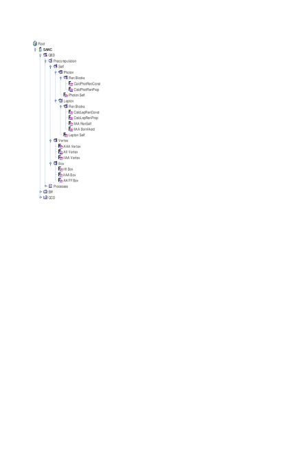
Figure 2: Precomputation in QED part.

It is worth emphasizing that at the precomputation phase it is not necessary to distinguish the process channel. While computing one-loop diagrams all 4-momenta are considered as incoming. In the derived expressions (say for the scalar form factors) any required channel is obtained by means of an appropriate permutation of arguments (say of Mandelstam variables $s,t,u$).

The Fig. 2 shows the fully open menu for “Precomputation” in the QED branch of SANC.

It consists of Self (Energies), Vertex and Box submenus. Self energies, in turn, are subdivided into Photon and Lepton submenus. They are further subdivided into calculation of diagrams themselves: Photon Self and Lepton Self. Precomputed and stored one-loop diagrams are used for calculation of corresponding renormalization constants: CalcPhotRenConst and CalcLepRenConsts, which are also stored. Altogether they are used for the calculation of renormalized propagators: CalcPhotRenProp and CalcLepRenProp. The latter is used to calculate the renormalized self energy 4-leg diagram for Compton scattering in QED llAA RenSelf. The file llbb Bornlikect computes Born-like counterterms (see Section 3.2.3).

Vertex consists of 3-photon-leg AAA, photon-2 lepton All and 4-leg vertices for NC $llAA$ Compton-like QED processes (any channel, see Section 3.3.3).

Box is represented by the NC 2-photon exchange 4-lepton-leg box (direct and crossed) llll Box (see Section 3.4.1) and by the two topologies (T2 and T4) of boxes appearing in Compton-like processes llAA Box (see Section 3.4.2). Finally, the file AA FF Box transforms results obtained by llll Box into the scalar form factors of a $4l$ process.

The tree of “Precomputation” in the EW part, which is shown in Fig. 3, has many more branches.

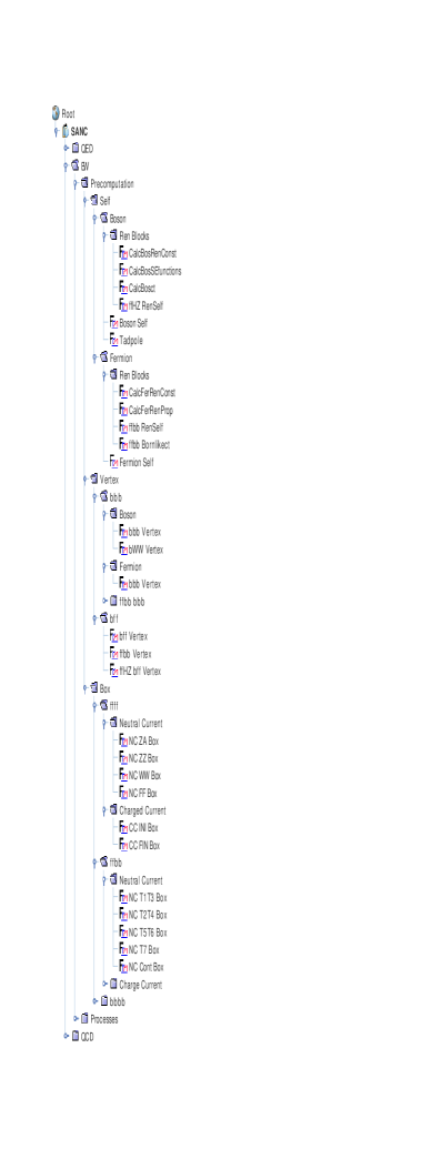
Figure 3: Precomputation in EW part.

It also consists of Self, Vertex and Box sub-items.

Self energies are subdivided into Boson and Fermion submenus. They are further subdivided into calculation of diagrams themselves: Boson Self and Tadpole (section 3.2.1) and Fermion Self (section 3.2.2). Precomputed and stored one-loop diagrams are used to calculate the corresponding renormalization constants: CalcBosRenConst and CalcFerRenConsts, which are also stored. They are all used to calculate the ingredients of renormalized bosonic propagators: CalcBosSEfunctions and CalcBosct and renormalized fermionic propagators CalcFerRenProp. The latter is used to calculate the renormalized self energy 4-leg diagram for $ffbb$ processes by ffbb RenSelf; ffbb Bornlikect computes Born-like counterterms (section 3.2.3).

Vertex consists of 3-boson-leg bbb and boson-2-fermion bff vertices. Vertices bbb contain Bosonic and Fermionic components and bbb vertices for ffbb processes (closed here). The former is further subdivided into any neutral leg bbb Vertex and in particular any neutral boson to $W^{+}W^{-}$ bWW Vertex (section 3.3.2). Vertices bff are subdivided into any $bff$ 3-leg vertices and 4-leg vertices for NC $ffbb$ processes (section 3.3.1).

Box is subdivided into three large classes: ffff, ffbb and bbbb each of them is subdivided further into NC and CC boxes. The ffff class contains a rich collection of 4-fermion-leg NC and CC boxes, direct and crossed, (section 3.4.1). The ffbb family is presented by now by seven topologies of boxes (NC T1–T7 Box) appearing in NC $ffbb$ processes (section 3.4.2).

The file NC FF Box transforms results obtained by ffff into the scalar form factors of a $4f$ process, while NC Cont Box realizes some further manipulations with NC $ffbb$ boxes (section 3.4.2).

The files intended for Charged Current boxes for $ffbb$ processes and for bbbb boxes exist but are not added for the time being.

3.2 Self energies

3.2.1 Bosonic self energy

Self energies are the simplest one-loop diagrams. There are three topologies of bosonic self-energy:

$$\begin{array}[]{ccc}\vbox{\hbox{ \begin{picture}(150.0,80.0)(0.0,0.0) \put(0.0,0.0){} \put(0.0,0.0){} \put(0.0,0.0){} \put(0.0,0.0){} \par \put(0.0,0.0){} \put(0.0,0.0){} \par \put(0.0,0.0){} \put(0.0,0.0){} \par \raise 40.0pt\hbox to0.0pt{\kern 26.5pt\makebox(0.0,0.0)[lb]{ $\mu$}\hss} \ignorespaces \raise 40.0pt\hbox to0.0pt{\kern 89.0pt\makebox(0.0,0.0)[lb]{ $\nu$}\hss} \ignorespaces \par \raise 57.0pt\hbox to0.0pt{\kern 88.0pt\makebox(0.0,0.0)[lb]{ $\lambda$}\hss} \ignorespaces \raise 39.0pt\hbox to0.0pt{\kern 76.0pt\makebox(0.0,0.0)[lb]{ $\delta$}\hss} \ignorespaces \raise 57.0pt\hbox to0.0pt{\kern 28.0pt\makebox(0.0,0.0)[lb]{ $\alpha$}\hss} \ignorespaces \raise 40.0pt\hbox to0.0pt{\kern 42.0pt\makebox(0.0,0.0)[lb]{ $\beta$}\hss} \ignorespaces \par \raise 49.0pt\hbox to0.0pt{\kern-12.0pt\makebox(0.0,0.0)[lb]{ $i$}\hss} \ignorespaces \raise 49.0pt\hbox to0.0pt{\kern 130.0pt\makebox(0.0,0.0)[lb]{ $j$}\hss} \ignorespaces \par \raise 62.0pt\hbox to0.0pt{\kern 59.0pt\makebox(0.0,0.0)[lb]{ $l$}\hss} \ignorespaces \raise 30.0pt\hbox to0.0pt{\kern 59.0pt\makebox(0.0,0.0)[lb]{ $k$}\hss} \ignorespaces \par \raise 10.0pt\hbox to0.0pt{\kern 38.0pt\makebox(0.0,0.0)[lb]{ $-q-p_{1}$}\hss} \ignorespaces \raise 85.0pt\hbox to0.0pt{\kern 59.0pt\makebox(0.0,0.0)[lb]{ $q$}\hss} \ignorespaces \raise 35.0pt\hbox to0.0pt{\kern 12.0pt\makebox(0.0,0.0)[lb]{ $p_{1}$}\hss} \ignorespaces \raise 35.0pt\hbox to0.0pt{\kern 98.0pt\makebox(0.0,0.0)[lb]{$-p_{1}$}\hss} \ignorespaces \par \put(0.0,0.0){} \put(0.0,0.0){} \raise-5.0pt\hbox to0.0pt{\kern 15.0pt\makebox(0.0,0.0)[lb]{i) Bosonic component}\hss} \ignorespaces \end{picture}}}&&\vbox{\hbox{ \begin{picture}(150.0,80.0)(0.0,0.0)\par \put(0.0,0.0){} \put(0.0,0.0){} \par \put(0.0,0.0){} \par \put(0.0,0.0){} \put(0.0,0.0){} \par \put(0.0,0.0){} \par \put(0.0,0.0){} \put(0.0,0.0){} \par \raise 40.0pt\hbox to0.0pt{\kern 26.5pt\makebox(0.0,0.0)[lb]{ $\mu$}\hss} \ignorespaces \raise 40.0pt\hbox to0.0pt{\kern 89.0pt\makebox(0.0,0.0)[lb]{ $\nu$}\hss} \ignorespaces \par \raise 10.0pt\hbox to0.0pt{\kern 38.0pt\makebox(0.0,0.0)[lb]{ $-q-p_{1}$}\hss} \ignorespaces \raise 85.0pt\hbox to0.0pt{\kern 59.0pt\makebox(0.0,0.0)[lb]{ $q$}\hss} \ignorespaces \raise 62.0pt\hbox to0.0pt{\kern 59.0pt\makebox(0.0,0.0)[lb]{ $l$}\hss} \ignorespaces \raise 30.0pt\hbox to0.0pt{\kern 59.0pt\makebox(0.0,0.0)[lb]{ $k$}\hss} \ignorespaces \par \raise 49.0pt\hbox to0.0pt{\kern-12.0pt\makebox(0.0,0.0)[lb]{ $i$}\hss} \ignorespaces \raise 49.0pt\hbox to0.0pt{\kern 130.0pt\makebox(0.0,0.0)[lb]{ $j$}\hss} \ignorespaces \par \raise 35.0pt\hbox to0.0pt{\kern 12.0pt\makebox(0.0,0.0)[lb]{ $p_{1}$}\hss} \ignorespaces \raise 35.0pt\hbox to0.0pt{\kern 98.0pt\makebox(0.0,0.0)[lb]{$-p_{1}$}\hss} \ignorespaces \put(0.0,0.0){} \put(0.0,0.0){} \raise-5.0pt\hbox to0.0pt{\kern 15.0pt\makebox(0.0,0.0)[lb]{ii) Fermionic component}\hss} \ignorespaces \end{picture}}}\end{array}$$

Figure 4: Two point diagrams.

Figure 5: One point bosonic diagrams.

$$\begin{array}[]{ccc}\vbox{ \hbox{ \begin{picture}(150.0,80.0)(0.0,0.0)\par \put(0.0,0.0){} \par \put(0.0,0.0){} \put(0.0,0.0){} \par \put(0.0,0.0){} \put(0.0,0.0){} \par \put(0.0,0.0){} \put(0.0,0.0){} \par \put(0.0,0.0){} \put(0.0,0.0){} \put(0.0,0.0){} \put(0.0,0.0){} \put(0.0,0.0){} \put(0.0,0.0){} \par \raise 33.0pt\hbox to0.0pt{\kern 72.0pt\makebox(0.0,0.0)[lb]{$\beta$}\hss} \ignorespaces \raise 33.0pt\hbox to0.0pt{\kern 54.0pt\makebox(0.0,0.0)[lb]{$\alpha$}\hss} \ignorespaces \par \raise-26.0pt\hbox to0.0pt{\kern 72.0pt\makebox(0.0,0.0)[lb]{$\nu$}\hss} \ignorespaces \raise-26.0pt\hbox to0.0pt{\kern 52.0pt\makebox(0.0,0.0)[lb]{$\mu$}\hss} \ignorespaces \par \raise-18.0pt\hbox to0.0pt{\kern-9.0pt\makebox(0.0,0.0)[lb]{$i$}\hss} \ignorespaces \raise-18.0pt\hbox to0.0pt{\kern 134.0pt\makebox(0.0,0.0)[lb]{$j$}\hss} \ignorespaces \par \raise-30.0pt\hbox to0.0pt{\kern 16.0pt\makebox(0.0,0.0)[lb]{$p_{1}$}\hss} \ignorespaces \raise-30.0pt\hbox to0.0pt{\kern 98.0pt\makebox(0.0,0.0)[lb]{$-p_{1}$}\hss} \ignorespaces \par \raise 62.0pt\hbox to0.0pt{\kern 64.0pt\makebox(0.0,0.0)[lb]{$l$}\hss} \ignorespaces \raise 85.0pt\hbox to0.0pt{\kern 64.0pt\makebox(0.0,0.0)[lb]{$q$}\hss} \ignorespaces \par \raise 12.0pt\hbox to0.0pt{\kern 50.0pt\makebox(0.0,0.0)[lb]{$(\delta)$}\hss} \ignorespaces \raise-10.0pt\hbox to0.0pt{\kern 50.0pt\makebox(0.0,0.0)[lb]{$(\lambda)$}\hss} \ignorespaces \raise-50.0pt\hbox to0.0pt{\kern 15.0pt\makebox(0.0,0.0)[lb]{iv) Bosonic component}\hss} \ignorespaces \end{picture} } }&&\vbox{ \hbox{ \begin{picture}(150.0,80.0)(0.0,0.0)\par \put(0.0,0.0){} \par \put(0.0,0.0){} \put(0.0,0.0){} \par \put(0.0,0.0){} \par \put(0.0,0.0){} \put(0.0,0.0){} \par \put(0.0,0.0){} \put(0.0,0.0){} \put(0.0,0.0){} \put(0.0,0.0){} \put(0.0,0.0){} \put(0.0,0.0){} \par \raise-26.0pt\hbox to0.0pt{\kern 72.0pt\makebox(0.0,0.0)[lb]{$\nu$}\hss} \ignorespaces \raise-26.0pt\hbox to0.0pt{\kern 52.0pt\makebox(0.0,0.0)[lb]{$\mu$}\hss} \ignorespaces \par \raise-18.0pt\hbox to0.0pt{\kern-9.0pt\makebox(0.0,0.0)[lb]{$i$}\hss} \ignorespaces \raise-18.0pt\hbox to0.0pt{\kern 134.0pt\makebox(0.0,0.0)[lb]{$j$}\hss} \ignorespaces \par \raise-30.0pt\hbox to0.0pt{\kern 16.0pt\makebox(0.0,0.0)[lb]{$p_{1}$}\hss} \ignorespaces \raise-30.0pt\hbox to0.0pt{\kern 98.0pt\makebox(0.0,0.0)[lb]{$-p_{1}$}\hss} \ignorespaces \par \raise 62.0pt\hbox to0.0pt{\kern 64.0pt\makebox(0.0,0.0)[lb]{$l$}\hss} \ignorespaces \raise 85.0pt\hbox to0.0pt{\kern 64.0pt\makebox(0.0,0.0)[lb]{$q$}\hss} \ignorespaces \par \raise 12.0pt\hbox to0.0pt{\kern 50.0pt\makebox(0.0,0.0)[lb]{$(\delta)$}\hss} \ignorespaces \raise-10.0pt\hbox to0.0pt{\kern 50.0pt\makebox(0.0,0.0)[lb]{$(\lambda)$}\hss} \ignorespaces \raise-50.0pt\hbox to0.0pt{\kern 15.0pt\makebox(0.0,0.0)[lb]{v) Fermionic component}\hss} \ignorespaces \end{picture}}}\end{array}$$

Figure 6: Tadpoles.

For the first and the third topologies it is useful to distinguish bosonic and fermionic components.

All these diagrams are precomputed and stored in the BS.sav file. At user request they may be recomputed by a FORM program accessible via the menu sequence EW $\to$ Precomputation $\to$ Self $\to$ Boson $\to$ Boson Self. The five types of self energies are defined in the specific procedure Diagb(i,j) (see the definitions of procedure types in the Introduction).

To give an example of what the precomputation really does, we present a simplified version of a very similar module accessible via the menu sequence QED $\to$ Precomputation $\to$ Self $\to$ Photon $\to$ Photon Self. It starts with the defining expression vacpol for the photonic vacuum polarization, Fig.4 ii) and continues in five steps of calls to the intrinsic procedures (i) FeynmanRules, (ii) Diracizing, (iii) GammaTrace, (iv) Reduction and (v) Scalarizing described in Section 4.2. After steps 1-4) we show the intermediate results and after step 5) — the final result.

#include Declar.h
#call Globals()

g vacpol = -Tr*vert(+1,12,-12,mu,ii)*pr(12,q,ii)
              *vert(-1,12,-12,nu,ii)*pr(12,q+p1,ii)*int;
(i)
#call FeynmanRules(0)

vacpol =
+ den(1,mel,q)*den(1,mel,q+p1)*e^2*qel^2*int*Tr*
(-gd(ii,mu)*gd(ii,q)*gd(ii,nu)*i_*mel-gd(ii,mu)*gd(ii,q)*gd(ii,nu)*gd(ii,q)
 -gd(ii,mu)*gd(ii,q)*gd(ii,nu)*gd(ii,p1)+gd(ii,mu)*gd(ii,nu)*mel^2
 -gd(ii,mu)*gd(ii,nu)*gd(ii,q)*i_*mel-gd(ii,mu)*gd(ii,nu)*gd(ii,p1)*i_*mel );
(ii)
#call Diracizing(0)

vacpol =
+ den(1,mel,q)*den(1,mel,q+p1)*e^2*qel^2*int*Tr*
(-2*gd(ii,mu)*gd(ii,al1)*qf(al1)*qf(nu)-gd(ii,mu)*gd(ii,al1)*gd(ii,nu)*qf(al1)*i_*mel
 -gd(ii,mu)*gd(ii,al1)*gd(ii,nu)*gd(ii,p1)*qf(al1)+gd(ii,mu)*gd(ii,nu)*mel^2
 +gd(ii,mu)*gd(ii,nu)*q.q-gd(ii,mu)*gd(ii,nu)*gd(ii,p1)*i_*mel
 -gd(ii,mu)*gd(ii,nu)*gd(ii,al1)*qf(al1)*i_*mel );
(iii)
#call GammaTrace(1)

vacpol =
+ den(1,mel,q)*den(1,mel,q+p1)*e^2*qel^2*int*
( 4*d_(mu,nu)*mel^2+4*d_(mu,nu)*q.q+4*d_(mu,nu)*q.p1
 -4*qf(mu)*p1(nu)-8*qf(mu)*qf(nu)-4*qf(nu)*p1(mu) );
(iv)
#call Reduction(0)

vacpol =
+ p1(mu)*p1(nu)*e^2*qel^2*
(-8*b21(p1s,1,mel,1,mel)-8*b1(p1s,1,mel,1,mel))
 +d_(mu,nu)*e^2*qel^2*
(4*a0(1,mel)-8*b22(p1s,1,mel,1,mel)+4*b1(p1s,1,mel,1,mel)*p1s);
(v)
#call Scalarizing(0)

vacpol =
+ p1(mu)*p1(nu)*e^2*qel^2*
(-4/9-8/3*p1s^-1*mel^2-8/3*a0(1,mel)*p1s^-1+4/3*b0(p1s,1,mel,1,mel)
 -8/3*b0(p1s,1,mel,1,mel)*p1s^-1*mel^2 )
+ d_(mu,nu)*e^2*qel^2 *
( 4/9*p1s + 8/3*mel^2 + 8/3*a0(1,mel) - 4/3*b0(p1s,1,mel,1,mel)*p1s
 +8/3*b0(p1s,1,mel,1,mel)*mel^2 );

We continue describing the structure of the basic program Boson Self:
The calculation of all bosonic self-energies (diagram-by-diagram) is done by two calls to specific procedure CalcBos(i,j), with {$i=3,\,6$, $j=i$}, corresponding to the charged external bosons $W^{\pm}$ and $\phi^{\pm}$, four calls to CalcBos(i,j) with {$i=1,2,4,5$, $j=i$}, corresponding to $\gamma$, $Z$, $H$ and $\phi^{0}$, and one call to CalcBos(i,j) with {$i=2$, $j=1$}, corresponding to external bosons $Z$ and $\gamma$, respectively.

Procedure CalcBos(i,j) calls specific procedure Diagb(i,j) and seven intrinsic procedures:(i) FeynmanRules, (ii) GammaRight, (iii) Diracizing, (iv) GammaTrace, (v) Reduction, (vi) Sing and (vii) Scalarizing. The intrinsic procedures are described in Section 4.2.

At each call to procedure CalcBos(i,j), the diagrams Figs. 4, 5, 6 are calculated for twelve virtual fermions field indices $k,l$ running over $11,\,12\,\ldots\,22$ (corresponding to $\nu_{e}$, $e$, $u$, $d$, $\nu_{\mu}$, $\mu$, $c$, $s$, $\nu_{\tau}$, $\tau$, $t$ and $b$, respectively) and for ten virtual bosons $k,l=1,\,2,\,\ldots,\,10$, corresponding to $\gamma$, $Z$, $W^{\pm}$, $H$, $\phi^{0}$, $\phi^{\pm}$ and four Faddeev–Popov ghosts $X^{+}$,$X^{-}$, $Y_{\scriptscriptstyle{Z}}$, $Y_{\scriptscriptstyle{A}}$, respectively.

The topology of the self-energy diagrams is specified in procedure Diagb(i,j) in terms of the vertices and propagators of the diagrams. In the class of diagrams available at present, vertices are of two kinds: boson-fermion-fermion (Bff) and three-boson (BBB) vertices. The diagrams are computed in nested loops over all allowed field indices of the virtual particles.

Two more FORM programs are accessible via menu sequences
QED $\to$ Precomputation $\to$ Self $\to$ Photon $\to$ Boson Self $\to$ Photon Self and
EW $\to$ Precomputation $\to$ Self $\to$ Boson $\to$ Tadpoles.
They have very similar structures and compute respectively photonic self energy (vacuum polarization) in the QED tree of SANC and tadpole diagrams separately from self energies. The results are stored in PSqed.sav and TP.sav files, respectively.

Precomputed bosonic self-energies are used by the other FORM programs which calculate bosonic counterterms
EW $\to$ Precomputation $\to$ Self $\to$ Boson $\to$ Ren Blocks $\to$ CalcBosRenConst
and the photonic counterterm
QED $\to$ Precomputation $\to$ Self $\to$ Photon $\to$ CalcPhotRenConst
in the QED tree; bosonic self energy functions
EW $\to$ Precomputation $\to$ Self $\to$ Boson $\to$ Ren Blocks $\to$ CalcBosSEFunctions,
and the renormalized photonic propagator in the QED branch
QED $\to$ Precomputation $\to$ Self $\to$ Photon $\to$ CalcPhotRenProp.
Their results, in turn, are used by a FORM program which computes counter term blocks (crosses), see Fig. 15 of Ref. [9]. The latter is accessible via the chain
EW $\to$ Precomputation $\to$ Self $\to$ Boson $\to$ Ren Blocks $\to$ CalcBosct.

3.2.2 Fermionic self energy

There are two topologies of fermion self energy diagrams (two point diagrams Fig. 7 and tadpoles Fig. 8).

Figure 7: Two point diagrams.

$$\begin{array}[]{ccc}\vbox{ \hbox{ \begin{picture}(150.0,80.0)(0.0,0.0)\par \put(0.0,0.0){} \par \put(0.0,0.0){} \put(0.0,0.0){} \par \put(0.0,0.0){} \put(0.0,0.0){} \par \put(0.0,0.0){} \put(0.0,0.0){} \put(0.0,0.0){} \put(0.0,0.0){} \par \put(0.0,0.0){} \put(0.0,0.0){} \put(0.0,0.0){} \put(0.0,0.0){} \put(0.0,0.0){} \put(0.0,0.0){} \par \raise 33.0pt\hbox to0.0pt{\kern 72.0pt\makebox(0.0,0.0)[lb]{$\beta$}\hss} \ignorespaces \raise 33.0pt\hbox to0.0pt{\kern 54.0pt\makebox(0.0,0.0)[lb]{$\alpha$}\hss} \ignorespaces \par \raise-18.0pt\hbox to0.0pt{\kern-9.0pt\makebox(0.0,0.0)[lb]{$i$}\hss} \ignorespaces \raise-18.0pt\hbox to0.0pt{\kern 134.0pt\makebox(0.0,0.0)[lb]{$j$}\hss} \ignorespaces \par \raise-30.0pt\hbox to0.0pt{\kern 16.0pt\makebox(0.0,0.0)[lb]{$p_{1}$}\hss} \ignorespaces \raise-30.0pt\hbox to0.0pt{\kern 98.0pt\makebox(0.0,0.0)[lb]{$-p_{1}$}\hss} \ignorespaces \par \raise 62.0pt\hbox to0.0pt{\kern 64.0pt\makebox(0.0,0.0)[lb]{$l$}\hss} \ignorespaces \raise 85.0pt\hbox to0.0pt{\kern 64.0pt\makebox(0.0,0.0)[lb]{$q$}\hss} \ignorespaces \par \raise 12.0pt\hbox to0.0pt{\kern 50.0pt\makebox(0.0,0.0)[lb]{$(\delta)$}\hss} \ignorespaces \raise-10.0pt\hbox to0.0pt{\kern 50.0pt\makebox(0.0,0.0)[lb]{$(\lambda)$}\hss} \ignorespaces \raise-50.0pt\hbox to0.0pt{\kern 15.0pt\makebox(0.0,0.0)[lb]{ii) Bosonic component}\hss} \ignorespaces \end{picture} } }&&\vbox{ \hbox{ \begin{picture}(150.0,80.0)(0.0,0.0)\par \put(0.0,0.0){} \par \put(0.0,0.0){} \put(0.0,0.0){} \par \put(0.0,0.0){} \par \put(0.0,0.0){} \put(0.0,0.0){} \put(0.0,0.0){} \put(0.0,0.0){} \put(0.0,0.0){} \par \put(0.0,0.0){} \put(0.0,0.0){} \put(0.0,0.0){} \put(0.0,0.0){} \put(0.0,0.0){} \par \raise-18.0pt\hbox to0.0pt{\kern-9.0pt\makebox(0.0,0.0)[lb]{$i$}\hss} \ignorespaces \raise-18.0pt\hbox to0.0pt{\kern 134.0pt\makebox(0.0,0.0)[lb]{$j$}\hss} \ignorespaces \par \raise-30.0pt\hbox to0.0pt{\kern 16.0pt\makebox(0.0,0.0)[lb]{$p_{1}$}\hss} \ignorespaces \raise-30.0pt\hbox to0.0pt{\kern 98.0pt\makebox(0.0,0.0)[lb]{$-p_{1}$}\hss} \ignorespaces \par \raise 62.0pt\hbox to0.0pt{\kern 64.0pt\makebox(0.0,0.0)[lb]{$l$}\hss} \ignorespaces \raise 85.0pt\hbox to0.0pt{\kern 64.0pt\makebox(0.0,0.0)[lb]{$q$}\hss} \ignorespaces \par \raise 12.0pt\hbox to0.0pt{\kern 50.0pt\makebox(0.0,0.0)[lb]{$(\delta)$}\hss} \ignorespaces \raise-10.0pt\hbox to0.0pt{\kern 50.0pt\makebox(0.0,0.0)[lb]{$(\lambda)$}\hss} \ignorespaces \raise-50.0pt\hbox to0.0pt{\kern 15.0pt\makebox(0.0,0.0)[lb]{iii) Fermionic component}\hss} \ignorespaces \end{picture} } }\end{array}$$

Figure 8: Tadpoles.

These diagrams are precomputed and stored in the FS.sav file. They may be recomputed by a FORM program accessible via the menu sequence
EW $\to$ Precomputation $\to$ Self $\to$ Fermion $\to$ Fermion Self.
The three types of diagrams are defined in the specific procedure Diagf(i,j).

Structure of the program Fermion Self:
The calculation is done by 12 calls to specific procedure CalcFer(i,j), with $i=j=11,\,12\,\ldots,\,22$, corresponding to all fermions of four generations, respectively.

Procedure CalcFer(i,i) calls specific procedure Diagf(i,j) and seven intrinsic procedures (i) FeynmanRules, (ii) GammaRight, (iii) Diracizing, (iv) GammaTrace, (v) Reduction, (vi) Sing and (vii) Scalarizing, see Section 4.2.

At each call to procedure CalcFer(i,i), the diagrams Figs. 7 and 8 are calculated for twelve virtual fermions $i=11,\,12\,\ldots,\,22$ and only six virtual bosons $l=1,\,2,\,\ldots,\,6$, corresponding to $\gamma$, $Z$, $W^{\pm}$, $h$, $\phi^{0}$ and $\phi^{\pm}$, respectively, since Faddeev–Popov ghosts do not contribute here.

The topology of the self-energy diagrams is specified in procedure Diagf(i,j) in terms of the vertices and propagators of the diagrams as well as sign and combinatorial factors (sign(‘l’) and cft(‘l’)).

There is one more FORM program, accessible via the menu sequence
QED $\to$ Precomputation $\to$ Self $\to$ Lepton $\to$ Lepton Self
whose structure is very similar to program Fermion Self. It computes the leptonic self energy in the QED tree of SANC. The results are stored in LSqed.sav file. Precomputed fermionic self-energies are used by FORM programs which calculate fermionic counterterms
EW $\to$ Precomputation $\to$ Self $\to$ Fermion $\to$ Ren Blocks $\to$ CalcFerRenConst
and leptonic counterterms
QED $\to$ Precomputation $\to$ Self $\to$ Lepton $\to$ CalcLepRenConst.
Both fermionic self-energy diagrams and fermionic counterterms are used by FORM programs which compute the renormalized fermionic (leptonic in the QED branch) propagators
EW $\to$ Precomputation $\to$ Self $\to$ Fermion $\to$ Ren Blocks $\to$ CalcFerRenProp and
QED $\to$ Precomputation $\to$ Self $\to$ Lepton $\to$ CalcLepRenProp, respectively.

In the FORM code CalcLepRenProp we show the main steps of the calculations. The two latter codes end up demonstrating the vanishing of the renormalized propagator on the corresponding fermionic mass shell, as is required by the on-mass-shell (OMS) renormalization scheme, see Section 2.2 of [9].

3.2.3 Fermionic self energy for $ffbb$ processes

Moving to precomputation of the building blocks for $ffbb$ processes, we change our conventions. Now any object: self energy, vertex and box are considered to be 4-legs, rather than 2-, 3- and 4-legs respectively, as we did before. The main motivation for this change is our observation that vertices with off-shell fermions are inconvenient to treat and the resulting expressions are more compact if we consider 4-legs on-mass-shell building blocks instead of 3-legs off-shell. Accepting this convention for vertices, it is natural to treat self-energies also like 4-leg objects shown in Fig. 9:

$$\begin{array}[]{ccc}\vbox{\hbox{ \begin{picture}(132.0,132.0)(0.0,0.0)\par \put(0.0,0.0){} \par \put(0.0,0.0){} \put(0.0,0.0){} \par \put(0.0,0.0){} \par \put(0.0,0.0){} \put(0.0,0.0){} \put(0.0,0.0){} \put(0.0,0.0){} \put(0.0,0.0){} \par \put(0.0,0.0){} \put(0.0,0.0){} \put(0.0,0.0){} \par \put(0.0,0.0){} \put(0.0,0.0){} \par \raise 132.0pt\hbox to0.0pt{\kern-32.0pt\makebox(0.0,0.0)[lt]{\sf ii}\hss} \ignorespaces \raise 118.0pt\hbox to0.0pt{\kern 42.0pt\makebox(0.0,0.0)[lb]{$p$}\hss} \ignorespaces \raise 3.0pt\hbox to0.0pt{\kern 37.0pt\makebox(0.0,0.0)[lb]{$Q$}\hss} \ignorespaces \raise 106.0pt\hbox to0.0pt{\kern-15.0pt\makebox(0.0,0.0)[lb]{$\nu$}\hss} \ignorespaces \raise 105.0pt\hbox to0.0pt{\kern 60.0pt\makebox(0.0,0.0)[lb]{vu=typeFU}\hss} \ignorespaces \raise 18.0pt\hbox to0.0pt{\kern 60.0pt\makebox(0.0,0.0)[lb]{vd=typeFD}\hss} \ignorespaces \raise 137.0pt\hbox to0.0pt{\kern-42.0pt\makebox(0.0,0.0)[lb]{fu=typeIU}\hss} \ignorespaces \raise-12.0pt\hbox to0.0pt{\kern-42.0pt\makebox(0.0,0.0)[lb]{fd=typeID}\hss} \ignorespaces \raise 17.0pt\hbox to0.0pt{\kern-15.0pt\makebox(0.0,0.0)[lb]{$\mu$}\hss} \ignorespaces \raise 123.0pt\hbox to0.0pt{\kern-4.0pt\makebox(0.0,0.0)[lb]{$p_{1}$}\hss} \ignorespaces \raise 3.0pt\hbox to0.0pt{\kern-4.0pt\makebox(0.0,0.0)[lb]{$p_{2}$}\hss} \ignorespaces \raise-12.0pt\hbox to0.0pt{\kern 35.0pt\makebox(0.0,0.0)[lb]{a)}\hss} \ignorespaces \end{picture}}}&&\vbox{\hbox{ \begin{picture}(132.0,132.0)(0.0,0.0) \put(0.0,0.0){} \par \put(0.0,0.0){} \put(0.0,0.0){} \par \put(0.0,0.0){} \put(0.0,0.0){} \put(0.0,0.0){} \put(0.0,0.0){} \put(0.0,0.0){} \put(0.0,0.0){} \par \put(0.0,0.0){} \put(0.0,0.0){} \put(0.0,0.0){} \par \put(0.0,0.0){} \put(0.0,0.0){} \par \raise 132.0pt\hbox to0.0pt{\kern-32.0pt\makebox(0.0,0.0)[lt]{\sf ii}\hss} \ignorespaces \raise 118.0pt\hbox to0.0pt{\kern 42.0pt\makebox(0.0,0.0)[lb]{$Q$}\hss} \ignorespaces \raise 6.0pt\hbox to0.0pt{\kern 37.0pt\makebox(0.0,0.0)[lb]{$p$}\hss} \ignorespaces \raise 105.0pt\hbox to0.0pt{\kern-15.0pt\makebox(0.0,0.0)[lb]{$\mu$}\hss} \ignorespaces \raise 18.0pt\hbox to0.0pt{\kern 60.0pt\makebox(0.0,0.0)[lb]{vu=typeFU}\hss} \ignorespaces \raise 105.0pt\hbox to0.0pt{\kern 60.0pt\makebox(0.0,0.0)[lb]{vd=typeFD}\hss} \ignorespaces \raise 137.0pt\hbox to0.0pt{\kern-42.0pt\makebox(0.0,0.0)[lb]{fu=typeIU}\hss} \ignorespaces \raise-12.0pt\hbox to0.0pt{\kern-42.0pt\makebox(0.0,0.0)[lb]{fd=typeID}\hss} \ignorespaces \raise 18.0pt\hbox to0.0pt{\kern-15.0pt\makebox(0.0,0.0)[lb]{$\nu$}\hss} \ignorespaces \raise 123.0pt\hbox to0.0pt{\kern-4.0pt\makebox(0.0,0.0)[lb]{$p_{1}$}\hss} \ignorespaces \raise 3.0pt\hbox to0.0pt{\kern-4.0pt\makebox(0.0,0.0)[lb]{$p_{2}$}\hss} \ignorespaces \raise-12.0pt\hbox to0.0pt{\kern 35.0pt\makebox(0.0,0.0)[lb]{b)}\hss} \ignorespaces \end{picture}}}\end{array}$$

Figure 9: Self energy $ffbb$ diagrams.

Here the blob at the fermion propagator denotes the sum of all self-energy diagrams described in Section 3.2.2. These self energies are precomputed by a FORM program accessible via the menu sequence
EW $\to$ Precomputation $\to$ Self $\to$ Fermion $\to$ Ren Blocks $\to$ ffbb RenSelf.

The required CPU time is still very short, and at user request they may be re-computed. The two types of self energies are defined in the specific procedures CalcFerSEt(fu,fd,vd,vu) and CalcFerSEu(fu,fd,vu,vd), which use renormalized fermionic propagators precomputed by CalcFerRenProp. Note that the labels ‘t’ and ‘u’ are associated with the Mandelstam variables $t,u$, see Section 2.4.

Both $t$ and $u$ channel procedures call intrinsic procedures FeynmanRules, GammaRight and p2I where the latter, together with several id’s in between, performs obvious identities and change of variables.

Computed diagrams FSEt‘fu’‘fd’‘vd’‘vu’‘jl’‘k1’ and FSEu‘fu’‘fd’‘vu’‘vd’‘jl’‘k1’ are stored in the file
ffbbSelfxi‘xi’‘fu’‘fd’‘vu’‘vd’.sav, where the predefined parameter ‘xi’ has the following meaning:

#define xi "0" / * .eq.0 to test gauge invariance / * .eq.1 to work in xi=1 gauge

This option is introduced mostly to save CPU time since calculation in the xi=1 gauge are much faster than in the $R_{\xi}$ gauge. However, it is always appealing to see the explicit cancellation of gauge parameters. That is why we try to maintain option xi ”0” as long as possible even though in some cases it is extremely time consuming.

There is a similar FORM program in the QED part, accessible via the menu sequence
QED $\to$ Precomputation $\to$ Self $\to$ Lepton $\to$ Ren Blocks $\to$ llAA RenSelf.

Furthermore, the code, accessible via menu sequence:
EW $\to$ Precomputation $\to$ Self $\to$ Fermion $\to$ Ren Blocks $\to$ ffbb Bornlikect
computes contributions from four diagrams similar to Fig. 9, in which the self energy blob at the fermion propagator is replaced by counterterm ‘crosses’ (one for each of the four diagrams at each vertex with indices $\mu$ and $\nu$, similar to Fig. 12). The result is stored in the file ffbbBornlikectxi‘xi’‘fu’‘fd’‘vu’‘vd’.sav.

The file from QED $\to$ Precomputation $\to$ Self $\to$ Lepton $\to$ Ren Blocks $\to$ ffAA Bornlikect does the same job in the QED part.

3.3 One-loop vertices

The current SANC version has all $bf\bar{f}$ and $bbb$ 3-leg SM vertices.

3.3.1 $bf\bar{f}$ vertices

There are two topologies of $bf\bar{f}$ vertices: FBF and BFB:

$$\begin{array}[]{ccc}\vbox{\hbox{ \begin{picture}(132.0,132.0)(20.0,0.0)\par \put(0.0,0.0){} \put(0.0,0.0){} \raise 64.0pt\hbox to0.0pt{\kern-72.0pt\makebox(0.0,0.0)[lb]{$i=$typeB}\hss} \ignorespaces \raise 76.0pt\hbox to0.0pt{\kern-22.0pt\makebox(0.0,0.0)[lb]{$Q=-p_{1}-p_{2}$}\hss} \ignorespaces \par \raise 75.0pt\hbox to0.0pt{\kern 61.0pt\makebox(0.0,0.0)[lb]{$k_{3}$}\hss} \ignorespaces \raise 52.0pt\hbox to0.0pt{\kern 61.0pt\makebox(0.0,0.0)[lb]{$k_{1}$}\hss} \ignorespaces \raise 66.0pt\hbox to0.0pt{\kern 75.0pt\makebox(0.0,0.0)[lb]{$k_{2}$}\hss} \ignorespaces \par \raise 55.0pt\hbox to0.0pt{\kern 35.0pt\makebox(0.0,0.0)[lb]{ $\mu$}\hss} \ignorespaces \raise 22.0pt\hbox to0.0pt{\kern 90.0pt\makebox(0.0,0.0)[lb]{ $\beta$}\hss} \ignorespaces \raise 105.0pt\hbox to0.0pt{\kern 90.0pt\makebox(0.0,0.0)[lb]{ $\alpha$}\hss} \ignorespaces \par \put(0.0,0.0){} \par \put(0.0,0.0){} \put(0.0,0.0){} \par \raise 37.0pt\hbox to0.0pt{\kern 43.0pt\makebox(0.0,0.0)[lb]{$-q$}\hss} \ignorespaces \raise 93.0pt\hbox to0.0pt{\kern 3.0pt\makebox(0.0,0.0)[lb]{$q+p_{1}+p_{2}$}\hss} \ignorespaces \par \put(0.0,0.0){} \put(0.0,0.0){} \par \put(0.0,0.0){} \put(0.0,0.0){} \put(0.0,0.0){} \par \put(0.0,0.0){} \put(0.0,0.0){} \put(0.0,0.0){} \par \put(0.0,0.0){} \raise 132.0pt\hbox to0.0pt{\kern 114.0pt\makebox(0.0,0.0)[lb]{$j=$typeU}\hss} \ignorespaces \raise 0.0pt\hbox to0.0pt{\kern 114.0pt\makebox(0.0,0.0)[lb]{$l=$typeD}\hss} \ignorespaces \raise 128.0pt\hbox to0.0pt{\kern 82.0pt\makebox(0.0,0.0)[lb]{$p_{2}$}\hss} \ignorespaces \raise 3.0pt\hbox to0.0pt{\kern 82.0pt\makebox(0.0,0.0)[lb]{$p_{1}$}\hss} \ignorespaces \raise 66.0pt\hbox to0.0pt{\kern 98.0pt\makebox(0.0,0.0)[lb]{$q+p_{1}$}\hss} \ignorespaces \put(0.0,0.0){} \raise-10.0pt\hbox to0.0pt{\kern 0.0pt\makebox(0.0,0.0)[lb]{a) Topology FBF}\hss} \ignorespaces \end{picture}}}&\vspace*{5cm}\hfil&\vbox{\hbox{ \begin{picture}(132.0,132.0)(-40.0,0.0)\par \put(0.0,0.0){} \put(0.0,0.0){} \raise 64.0pt\hbox to0.0pt{\kern-72.0pt\makebox(0.0,0.0)[lb]{$i=$typeB}\hss} \ignorespaces \raise 76.0pt\hbox to0.0pt{\kern 5.0pt\makebox(0.0,0.0)[lb]{$Q$}\hss} \ignorespaces \par \raise 75.0pt\hbox to0.0pt{\kern 61.0pt\makebox(0.0,0.0)[lb]{$k_{3}$}\hss} \ignorespaces \raise 52.0pt\hbox to0.0pt{\kern 61.0pt\makebox(0.0,0.0)[lb]{$k_{1}$}\hss} \ignorespaces \raise 66.0pt\hbox to0.0pt{\kern 75.0pt\makebox(0.0,0.0)[lb]{$k_{2}$}\hss} \ignorespaces \par \raise 57.0pt\hbox to0.0pt{\kern 30.0pt\makebox(0.0,0.0)[lb]{$\mu$}\hss} \ignorespaces \raise 78.0pt\hbox to0.0pt{\kern 39.0pt\makebox(0.0,0.0)[lb]{$\mu_{3}$}\hss} \ignorespaces \raise 50.0pt\hbox to0.0pt{\kern 39.0pt\makebox(0.0,0.0)[lb]{$\mu_{1}$}\hss} \ignorespaces \raise 22.0pt\hbox to0.0pt{\kern 93.0pt\makebox(0.0,0.0)[lb]{$\beta$}\hss} \ignorespaces \raise 105.0pt\hbox to0.0pt{\kern 93.0pt\makebox(0.0,0.0)[lb]{$\alpha$}\hss} \ignorespaces \par \put(0.0,0.0){} \par \put(0.0,0.0){} \put(0.0,0.0){} \par \raise 37.0pt\hbox to0.0pt{\kern 43.0pt\makebox(0.0,0.0)[lb]{$-q$}\hss} \ignorespaces \raise 93.0pt\hbox to0.0pt{\kern 3.0pt\makebox(0.0,0.0)[lb]{$q+p_{1}+p_{2}$}\hss} \ignorespaces \par \put(0.0,0.0){} \put(0.0,0.0){} \put(0.0,0.0){} \put(0.0,0.0){} \put(0.0,0.0){} \put(0.0,0.0){} \put(0.0,0.0){} \put(0.0,0.0){} \par \put(0.0,0.0){} \raise 132.0pt\hbox to0.0pt{\kern 114.0pt\makebox(0.0,0.0)[lb]{$j=$typeU}\hss} \ignorespaces \raise 0.0pt\hbox to0.0pt{\kern 114.0pt\makebox(0.0,0.0)[lb]{$l=$typeD}\hss} \ignorespaces \raise 128.0pt\hbox to0.0pt{\kern 82.0pt\makebox(0.0,0.0)[lb]{$p_{2}$}\hss} \ignorespaces \raise 3.0pt\hbox to0.0pt{\kern 82.0pt\makebox(0.0,0.0)[lb]{$p_{1}$}\hss} \ignorespaces \raise 66.0pt\hbox to0.0pt{\kern 98.0pt\makebox(0.0,0.0)[lb]{$q+p_{1}$}\hss} \ignorespaces \put(0.0,0.0){} \raise-10.0pt\hbox to0.0pt{\kern 0.0pt\makebox(0.0,0.0)[lb]{b) Topology BFB}\hss} \ignorespaces \end{picture}}}\end{array}$$

Figure 10: $bff$ vertices.

These vertex diagrams are precomputed by a FORM program accessible via menu sequence
EW $\to$ Precomputation $\to$ Vertex $\to$ bff $\to$ bff Vertex.

At user request they may be recomputed. The two types of vertices are defined in the specific procedures FBF(i,j,l) and BFB(i,j,l), where the topologies of all vertices of the type of Fig. 10 are specified in nested loops over all allowed field indices of the virtual particles.

Structure of program bff Vertex
The calculation is done by a single call to specific procedure CalcVertex(‘typeB’,‘typeU’,‘typeD’), followed by a call to intrinsic procedure p2D.

The arguments typeB, typeU, and typeD are the field indices of the external particles, set in the command that starts this program: typeB is the incoming boson, typeU is the antifermion with incoming 4-momentum $p_{2}$, and typeD is the fermion with incoming 4-momentum $p_{1}$. For instance, to calculate the vertex for $Z\to u\bar{u}$ decay, typeB, typeU, and typeD are set equal to $2,\,13,\,13$, respectively. The results are stored in files V‘typeB’‘typeU’‘typeD’.sav.

Procedure CalcVertex(i,j,l) calls specific procedures FBF(i,j,l) and BFB(i,j,l) and the intrinsic procedures in the following sequence: FeynmanRules, GammaRight, Diracizing, Reduction, Diracizing, Pulling, Diraceq, Sing, Scalarizing, 2Qs, Masshell and Symmetrize. The intrinsic procedures are described in Section 4.2.

In the QED tree there is a similar entry
QED $\to$ Precomputation $\to$ Vertex $\to$ Aff $\to$ Aff Vertex,
which computes $\gamma l\bar{l}$ vertices for a lepton of a kind j=typeU=12,16,20. These vertices are defined in the specific procedure DiagVert(j). The results are stored in files Vqed‘typeU’.sav.

3.3.2 $bbb$ vertices

The bosonic component of three-boson vertices has four topologies shown in the following diagrams:

Figure 11: Four topologies for three-boson vertices.

These vertex diagrams are precomputed by a FORM program accessible through the chain of clicks
EW $\to$ Precomputation $\to$ Vertex $\to$ bbb $\to$ Boson $\to$ bvv Vertex.
They also may be recomputed at user request. The four topologies are defined in the specific procedures TribosVertT1(i,l,j).

Structure of program bvv Vertex
The calculation is done by a single call to specific procedure CalcTribosVertT14(‘typeB’,‘typeD’,‘typeU’) which calls first of all four topologies in Figs. 11 defined in specific procedures TribosVertTk(i,l,j), with $k=1,2,3,4$.

Just after that four specific procedures ClTribosVertTk(i,l,j) perform clusterizing of the computed diagrams. One should note that clusters have different meanings in SANC. Here clusterizing means nothing but summation over all virtual field indices, resulting in the dependence of cluster names only on external field indices.

After clusterizing, the usual calls of the intrinsic procedures follow: FeynmanRules, 2Qs, Reduction, 2Qs, Sing and Scalarizing.

The fermionic component of three-boson vertices has only one topology T1. The diagrams are defined in the specific procedure TribosVertf(i,l,j).

Structure of program Fermion $\to$ bbb Vertex
The calculation is done by a single call to specific procedure CalcTribosVert(‘typeB’,‘typeD’,‘typeU’) which at first calls the topology defined in the specific procedure TribosVertf(i,l,j). Next, specific procedure ClT1fer(i,l,j) performs clusterizing.

The calculation of the cluster is followed by calls of the intrinsic procedures: FeynmanRules, GammaLeft, Diracizing, GammaTrace, Reduction, Scalarizing, Sing, Scalprod and DivisionGramDet.

One may access a similar FORM code to precompute the HWW, ZWW and AWW vertices via sequence EW $\to$ Precomputation $\to$ Vertex $\to$ bbb $\to$ Boson $\to$ bWW Vertex.

3.3.3 Vertices for $ffbb$ processes

There are four blocks of vertices met in $ffbb$ processes where only diagrams with fermion exchange contribute at the Born level (we have also $ffZH$ process where there is the Born diagram with boson exchange, so-called Higgsstrahlung, but this process is not added to SANC v.1.00):

$$\begin{array}[]{ccc}\vbox{\hbox{ \begin{picture}(132.0,132.0)(0.0,0.0)\par \put(0.0,0.0){} \put(0.0,0.0){} \par \put(0.0,0.0){} \par \put(0.0,0.0){} \put(0.0,0.0){} \put(0.0,0.0){} \put(0.0,0.0){} \par \put(0.0,0.0){} \put(0.0,0.0){} \put(0.0,0.0){} \par \put(0.0,0.0){} \put(0.0,0.0){} \par \raise 132.0pt\hbox to0.0pt{\kern-32.0pt\makebox(0.0,0.0)[lt]{\sf ii}\hss} \ignorespaces \raise 118.0pt\hbox to0.0pt{\kern 42.0pt\makebox(0.0,0.0)[lb]{$p$}\hss} \ignorespaces \raise 3.0pt\hbox to0.0pt{\kern 37.0pt\makebox(0.0,0.0)[lb]{$Q$}\hss} \ignorespaces \raise 106.0pt\hbox to0.0pt{\kern-15.0pt\makebox(0.0,0.0)[lb]{$\nu$}\hss} \ignorespaces \raise 105.0pt\hbox to0.0pt{\kern 60.0pt\makebox(0.0,0.0)[lb]{vd=typeFD}\hss} \ignorespaces \raise 18.0pt\hbox to0.0pt{\kern 60.0pt\makebox(0.0,0.0)[lb]{vu=typeFU}\hss} \ignorespaces \raise 137.0pt\hbox to0.0pt{\kern-42.0pt\makebox(0.0,0.0)[lb]{fu=typeIU}\hss} \ignorespaces \raise-12.0pt\hbox to0.0pt{\kern-42.0pt\makebox(0.0,0.0)[lb]{fd=typeID}\hss} \ignorespaces \raise 17.0pt\hbox to0.0pt{\kern-15.0pt\makebox(0.0,0.0)[lb]{$\mu$}\hss} \ignorespaces \raise 123.0pt\hbox to0.0pt{\kern-4.0pt\makebox(0.0,0.0)[lb]{$p_{1}$}\hss} \ignorespaces \raise 3.0pt\hbox to0.0pt{\kern-4.0pt\makebox(0.0,0.0)[lb]{$p_{2}$}\hss} \ignorespaces \raise-25.0pt\hbox to0.0pt{\kern 35.0pt\makebox(0.0,0.0)[lb]{a)}\hss} \ignorespaces \end{picture}}}&&\vbox{\hbox{ \begin{picture}(132.0,132.0)(0.0,0.0) \put(0.0,0.0){} \put(0.0,0.0){} \par \put(0.0,0.0){} \put(0.0,0.0){} \put(0.0,0.0){} \put(0.0,0.0){} \put(0.0,0.0){} \par \put(0.0,0.0){} \put(0.0,0.0){} \put(0.0,0.0){} \par \put(0.0,0.0){} \put(0.0,0.0){} \par \raise 132.0pt\hbox to0.0pt{\kern-32.0pt\makebox(0.0,0.0)[lt]{\sf ii}\hss} \ignorespaces \raise 118.0pt\hbox to0.0pt{\kern 42.0pt\makebox(0.0,0.0)[lb]{$Q$}\hss} \ignorespaces \raise 6.0pt\hbox to0.0pt{\kern 37.0pt\makebox(0.0,0.0)[lb]{$p$}\hss} \ignorespaces \raise 105.0pt\hbox to0.0pt{\kern-15.0pt\makebox(0.0,0.0)[lb]{$\mu$}\hss} \ignorespaces \raise 18.0pt\hbox to0.0pt{\kern 60.0pt\makebox(0.0,0.0)[lb]{vd=typeFD}\hss} \ignorespaces \raise 105.0pt\hbox to0.0pt{\kern 60.0pt\makebox(0.0,0.0)[lb]{vu=typeFU}\hss} \ignorespaces \raise 137.0pt\hbox to0.0pt{\kern-42.0pt\makebox(0.0,0.0)[lb]{fu=typeIU}\hss} \ignorespaces \raise-12.0pt\hbox to0.0pt{\kern-42.0pt\makebox(0.0,0.0)[lb]{fd=typeID}\hss} \ignorespaces \raise 18.0pt\hbox to0.0pt{\kern-15.0pt\makebox(0.0,0.0)[lb]{$\nu$}\hss} \ignorespaces \raise 123.0pt\hbox to0.0pt{\kern-4.0pt\makebox(0.0,0.0)[lb]{$p_{1}$}\hss} \ignorespaces \raise 3.0pt\hbox to0.0pt{\kern-4.0pt\makebox(0.0,0.0)[lb]{$p_{2}$}\hss} \ignorespaces \raise-25.0pt\hbox to0.0pt{\kern 35.0pt\makebox(0.0,0.0)[lb]{b)}\hss} \ignorespaces \end{picture}}}\\[113.81102pt] \vbox{\hbox{ \begin{picture}(132.0,132.0)(0.0,0.0) \put(0.0,0.0){} \put(0.0,0.0){} \par \put(0.0,0.0){} \par \put(0.0,0.0){} \put(0.0,0.0){} \put(0.0,0.0){} \put(0.0,0.0){} \par \put(0.0,0.0){} \put(0.0,0.0){} \put(0.0,0.0){} \par \put(0.0,0.0){} \put(0.0,0.0){} \par \raise 132.0pt\hbox to0.0pt{\kern-32.0pt\makebox(0.0,0.0)[lt]{\sf ii}\hss} \ignorespaces \raise 118.0pt\hbox to0.0pt{\kern 42.0pt\makebox(0.0,0.0)[lb]{$p$}\hss} \ignorespaces \raise 3.0pt\hbox to0.0pt{\kern 37.0pt\makebox(0.0,0.0)[lb]{$Q$}\hss} \ignorespaces \raise 106.0pt\hbox to0.0pt{\kern-15.0pt\makebox(0.0,0.0)[lb]{$\nu$}\hss} \ignorespaces \raise 105.0pt\hbox to0.0pt{\kern 60.0pt\makebox(0.0,0.0)[lb]{vd=typeFD}\hss} \ignorespaces \raise 18.0pt\hbox to0.0pt{\kern 60.0pt\makebox(0.0,0.0)[lb]{vu=typeFU}\hss} \ignorespaces \raise 137.0pt\hbox to0.0pt{\kern-42.0pt\makebox(0.0,0.0)[lb]{fu=typeIU}\hss} \ignorespaces \raise-12.0pt\hbox to0.0pt{\kern-42.0pt\makebox(0.0,0.0)[lb]{fd=typeID}\hss} \ignorespaces \raise 17.0pt\hbox to0.0pt{\kern-15.0pt\makebox(0.0,0.0)[lb]{$\mu$}\hss} \ignorespaces \raise 123.0pt\hbox to0.0pt{\kern-4.0pt\makebox(0.0,0.0)[lb]{$p_{1}$}\hss} \ignorespaces \raise 3.0pt\hbox to0.0pt{\kern-4.0pt\makebox(0.0,0.0)[lb]{$p_{2}$}\hss} \ignorespaces \raise-25.0pt\hbox to0.0pt{\kern 35.0pt\makebox(0.0,0.0)[lb]{c)}\hss} \ignorespaces \end{picture}}}&&\vbox{\hbox{ \begin{picture}(132.0,132.0)(0.0,0.0) \put(0.0,0.0){} \put(0.0,0.0){} \par \put(0.0,0.0){} \put(0.0,0.0){} \put(0.0,0.0){} \put(0.0,0.0){} \put(0.0,0.0){} \par \put(0.0,0.0){} \put(0.0,0.0){} \put(0.0,0.0){} \par \put(0.0,0.0){} \put(0.0,0.0){} \par \raise 132.0pt\hbox to0.0pt{\kern-32.0pt\makebox(0.0,0.0)[lt]{\sf ii}\hss} \ignorespaces \raise 118.0pt\hbox to0.0pt{\kern 42.0pt\makebox(0.0,0.0)[lb]{$Q$}\hss} \ignorespaces \raise 6.0pt\hbox to0.0pt{\kern 37.0pt\makebox(0.0,0.0)[lb]{$p$}\hss} \ignorespaces \raise 105.0pt\hbox to0.0pt{\kern-15.0pt\makebox(0.0,0.0)[lb]{$\mu$}\hss} \ignorespaces \raise 18.0pt\hbox to0.0pt{\kern 60.0pt\makebox(0.0,0.0)[lb]{vd=typeFD}\hss} \ignorespaces \raise 105.0pt\hbox to0.0pt{\kern 60.0pt\makebox(0.0,0.0)[lb]{vu=typeFU}\hss} \ignorespaces \raise 137.0pt\hbox to0.0pt{\kern-42.0pt\makebox(0.0,0.0)[lb]{fu=typeIU}\hss} \ignorespaces \raise-12.0pt\hbox to0.0pt{\kern-42.0pt\makebox(0.0,0.0)[lb]{fd=typeID}\hss} \ignorespaces \raise 18.0pt\hbox to0.0pt{\kern-15.0pt\makebox(0.0,0.0)[lb]{$\nu$}\hss} \ignorespaces \raise 123.0pt\hbox to0.0pt{\kern-4.0pt\makebox(0.0,0.0)[lb]{$p_{1}$}\hss} \ignorespaces \raise 3.0pt\hbox to0.0pt{\kern-4.0pt\makebox(0.0,0.0)[lb]{$p_{2}$}\hss} \ignorespaces \raise-25.0pt\hbox to0.0pt{\kern 35.0pt\makebox(0.0,0.0)[lb]{d)}\hss} \ignorespaces \end{picture}}}\end{array}$$

Figure 12: Four $ffbb$ vertex diagrams.

The four building blocks are precomputed by a FORM program accessible via menu sequence:
EW $\to$ Precomputation $\to$ Vertex $\to$ bff $\to$ ffbb Vertex.

Structure of program ffbb Vertex
The calculation is done by $2\otimes 3$ calls to the following specific procedures:
CalcVert(‘typeFU’,‘typeID’,‘typeIU’,mu)                  — computes vertex blob with index $\mu$;
CalcVertmut(‘typeIU’,‘typeID’,‘typeFD’,‘typeFU’,mu) — computes diagram b);
CalcVertmuu(‘typeIU’,‘typeID’,‘typeFU’,‘typeFD’,mu) — computes diagram c);
CalcVert(‘typeFD’,‘typeID’,‘typeIU’,nu)                   — computes vertex blob with index $\nu$;
CalcVertnut(‘typeIU’,‘typeID’,‘typeFD’,‘typeFU’,nu)   — computes diagram d);
CalcVertnuu(‘typeIU’,‘typeID’,‘typeFU’,‘typeFD’,nu)   — computes diagram a).

The procedure CalcVert recomputes $bff$ vertices for given set ‘typeFU’,‘typeID’,‘typeIU’ and creates expressions vfbf‘vu’‘fd’‘fu’‘mu’‘k1’‘k2’‘k3’ and vbfb‘vu’‘fd’‘fu’‘mu’‘k1’‘k2’‘k3’ similar to those described in Section 3.3.1, but not applying intrinsic procedure Masshell since in the case under consideration one of fermions is off-shell. The four procedures CalcVertmut, CalcVertmuu, CalcVertnut and CalcVertnuu have very similar structures.

In each of four procedures the intrinsic procedures FeynmanRules, GammaRight, bpIdentities, p2m, p2I and p2p are called. Next follows an important shift of the virtual fermion 4-momenta to ‘real’ four momenta $p_{1},p_{2},p,Q$, and finally ExtMomentumWI is applied.

All the building blocks are clusterized by summation over virtual momenta in vertex loops (see discussion of clusterization in Section 3.4.2.).

Besides xi there are three more internally defined options: on (see Section 3.4.2 for more discussion about option on) and mf, mp, of which the latter two allow to neglect fermion masses.

#define on "1"
* .eq.0 photons are off mass-shell; .eq.1 photons are on  mass-shell
#define mf "0"
* .eq.0 fermion mass, pm(‘typeID’)=0;  .eq.1 it is not neglected
#define mp "0"
* .eq.0 partner mass, pm(‘typeIDp’)=0; .eq.1 it is not neglected

The result of this calculation is stored in the file
ffbbVertxi‘xi’on‘on’mf‘mf’mp‘mp’ ‘typeIU’‘typeID’‘typeFU’‘typeFD’.sav.

3.4 One-loop boxes

Approaching the description of precomputation of boxes, one should note that the world of boxes is much more rich and complex compared to self-energies and vertices. If for the latter case we still could profess the idea of allowing recomputation of all one-loop vertices needed for the process under consideration, then in the case of boxes we must change our strategy if the user wants to carry out some recomputation.

For boxes, the idea of precomputation becomes vitally important for realization of SANC project. As will be explained below, calculation of some boxes for some particular processes takes so much time that an external user should refrain from repeating precomputation. Furthermore, the richness of boxes requires more classification. Depending on the type of external lines (fermion or boson), we will distinguish three large classes of boxes: ffff, ffbb and bbbb.

3.4.1 Boxes for $ffff$ processes

The ffff boxes, which are met in the description of 4f processes, are of two topologies, direct and crossed, and are characterized by two fermionic currents ii and jj, coupled by two bosons with field indices k1 and k3; see Fig. 13 showing all the field indices (for external and virtual fields), types of external fermions typeXX, Lorenz indices and momentum flows for the direct and crossed topologies.

$$\begin{array}[]{ccc}\vbox{\hbox{ \begin{picture}(132.0,132.0)(0.0,0.0)\par \raise 137.0pt\hbox to0.0pt{\kern-42.0pt\makebox(0.0,0.0)[lb]{iu=typeIU}\hss} \ignorespaces \raise 132.0pt\hbox to0.0pt{\kern-32.0pt\makebox(0.0,0.0)[lt]{\sf ii}\hss} \ignorespaces \raise 105.0pt\hbox to0.0pt{\kern-15.0pt\makebox(0.0,0.0)[lb]{$\alpha$}\hss} \ignorespaces \raise 123.0pt\hbox to0.0pt{\kern-4.0pt\makebox(0.0,0.0)[lb]{$p_{1}$}\hss} \ignorespaces \put(0.0,0.0){} \put(0.0,0.0){} \par \raise 63.0pt\hbox to0.0pt{\kern 4.0pt\makebox(0.0,0.0)[lb]{$k_{2}$}\hss} \ignorespaces \raise 63.0pt\hbox to0.0pt{\kern-35.0pt\makebox(0.0,0.0)[lb]{$q+p_{1}$}\hss} \ignorespaces \put(0.0,0.0){} \put(0.0,0.0){} \put(0.0,0.0){} \put(0.0,0.0){} \par \raise-12.0pt\hbox to0.0pt{\kern-42.0pt\makebox(0.0,0.0)[lb]{id=typeID}\hss} \ignorespaces \raise 15.0pt\hbox to0.0pt{\kern-15.0pt\makebox(0.0,0.0)[lb]{$\beta$}\hss} \ignorespaces \raise 3.0pt\hbox to0.0pt{\kern-4.0pt\makebox(0.0,0.0)[lb]{$p_{2}$}\hss} \ignorespaces \put(0.0,0.0){} \put(0.0,0.0){} \par \raise 118.0pt\hbox to0.0pt{\kern 42.0pt\makebox(0.0,0.0)[lb]{$q$}\hss} \ignorespaces \put(0.0,0.0){} \put(0.0,0.0){} \raise 95.0pt\hbox to0.0pt{\kern 40.0pt\makebox(0.0,0.0)[lb]{$k_{1}$}\hss} \ignorespaces \par \raise 25.0pt\hbox to0.0pt{\kern 40.0pt\makebox(0.0,0.0)[lb]{$k_{3}$}\hss} \ignorespaces \put(0.0,0.0){} \put(0.0,0.0){} \raise 6.0pt\hbox to0.0pt{\kern 17.0pt\makebox(0.0,0.0)[lb]{$q+p_{1}+p_{2}$}\hss} \ignorespaces \par \raise 137.0pt\hbox to0.0pt{\kern 90.0pt\makebox(0.0,0.0)[lb]{fu=typeFU}\hss} \ignorespaces \raise 132.0pt\hbox to0.0pt{\kern 115.0pt\makebox(0.0,0.0)[lt]{\sf jj}\hss} \ignorespaces \raise 123.0pt\hbox to0.0pt{\kern 82.0pt\makebox(0.0,0.0)[lb]{$p_{4}$ }\hss} \ignorespaces \raise 105.0pt\hbox to0.0pt{\kern 95.0pt\makebox(0.0,0.0)[lb]{$\mu$}\hss} \ignorespaces \put(0.0,0.0){} \put(0.0,0.0){} \par \raise 63.0pt\hbox to0.0pt{\kern 98.0pt\makebox(0.0,0.0)[lb]{$q-p_{4}$}\hss} \ignorespaces \put(0.0,0.0){} \raise 63.0pt\hbox to0.0pt{\kern 74.0pt\makebox(0.0,0.0)[lb]{$k_{4}$}\hss} \ignorespaces \put(0.0,0.0){} \put(0.0,0.0){} \put(0.0,0.0){} \par \raise-12.0pt\hbox to0.0pt{\kern 90.0pt\makebox(0.0,0.0)[lb]{fd=typeFD}\hss} \ignorespaces \raise 20.0pt\hbox to0.0pt{\kern 95.0pt\makebox(0.0,0.0)[lb]{$\nu$ }\hss} \ignorespaces \raise 3.0pt\hbox to0.0pt{\kern 82.0pt\makebox(0.0,0.0)[lb]{$p_{3}$ }\hss} \ignorespaces \put(0.0,0.0){} \put(0.0,0.0){} \par \raise-30.0pt\hbox to0.0pt{\kern 35.0pt\makebox(0.0,0.0)[lb]{a) Direct}\hss} \ignorespaces \end{picture}}}&&\vbox{\hbox{ \begin{picture}(132.0,132.0)(0.0,0.0)\par \raise 137.0pt\hbox to0.0pt{\kern-42.0pt\makebox(0.0,0.0)[lb]{iu=typeIU}\hss} \ignorespaces \raise 132.0pt\hbox to0.0pt{\kern-32.0pt\makebox(0.0,0.0)[lt]{\sf ii}\hss} \ignorespaces \raise 105.0pt\hbox to0.0pt{\kern-15.0pt\makebox(0.0,0.0)[lb]{$\alpha$}\hss} \ignorespaces \raise 123.0pt\hbox to0.0pt{\kern-4.0pt\makebox(0.0,0.0)[lb]{$p_{1}$}\hss} \ignorespaces \put(0.0,0.0){} \put(0.0,0.0){} \par \raise 63.0pt\hbox to0.0pt{\kern 4.0pt\makebox(0.0,0.0)[lb]{$k_{2}$}\hss} \ignorespaces \raise 63.0pt\hbox to0.0pt{\kern-35.0pt\makebox(0.0,0.0)[lb]{$q+p_{1}$}\hss} \ignorespaces \put(0.0,0.0){} \put(0.0,0.0){} \put(0.0,0.0){} \put(0.0,0.0){} \par \raise-12.0pt\hbox to0.0pt{\kern-42.0pt\makebox(0.0,0.0)[lb]{id=typeID}\hss} \ignorespaces \raise 15.0pt\hbox to0.0pt{\kern-15.0pt\makebox(0.0,0.0)[lb]{$\beta$}\hss} \ignorespaces \raise 3.0pt\hbox to0.0pt{\kern-4.0pt\makebox(0.0,0.0)[lb]{$p_{2}$}\hss} \ignorespaces \put(0.0,0.0){} \put(0.0,0.0){} \par \raise 118.0pt\hbox to0.0pt{\kern 42.0pt\makebox(0.0,0.0)[lb]{$q$}\hss} \ignorespaces \put(0.0,0.0){} \put(0.0,0.0){} \raise 95.0pt\hbox to0.0pt{\kern 40.0pt\makebox(0.0,0.0)[lb]{$k_{1}$}\hss} \ignorespaces \par \raise 25.0pt\hbox to0.0pt{\kern 40.0pt\makebox(0.0,0.0)[lb]{$k_{3}$}\hss} \ignorespaces \put(0.0,0.0){} \put(0.0,0.0){} \raise 6.0pt\hbox to0.0pt{\kern 17.0pt\makebox(0.0,0.0)[lb]{$q+p_{1}+p_{2}$}\hss} \ignorespaces \par \raise 137.0pt\hbox to0.0pt{\kern 90.0pt\makebox(0.0,0.0)[lb]{fd=typeFD}\hss} \ignorespaces \raise 132.0pt\hbox to0.0pt{\kern 115.0pt\makebox(0.0,0.0)[lt]{\sf jj}\hss} \ignorespaces \raise 123.0pt\hbox to0.0pt{\kern 82.0pt\makebox(0.0,0.0)[lb]{$p_{3}$}\hss} \ignorespaces \raise 105.0pt\hbox to0.0pt{\kern 95.0pt\makebox(0.0,0.0)[lb]{$\nu$}\hss} \ignorespaces \put(0.0,0.0){} \put(0.0,0.0){} \par \raise 63.0pt\hbox to0.0pt{\kern 98.0pt\makebox(0.0,0.0)[lb]{$q-p_{3}$}\hss} \ignorespaces \put(0.0,0.0){} \raise 63.0pt\hbox to0.0pt{\kern 75.0pt\makebox(0.0,0.0)[lb]{$k_{4}$}\hss} \ignorespaces \put(0.0,0.0){} \put(0.0,0.0){} \put(0.0,0.0){} \par \raise-12.0pt\hbox to0.0pt{\kern 90.0pt\makebox(0.0,0.0)[lb]{fu=typeFU}\hss} \ignorespaces \raise 20.0pt\hbox to0.0pt{\kern 95.0pt\makebox(0.0,0.0)[lb]{$\mu$}\hss} \ignorespaces \raise 3.0pt\hbox to0.0pt{\kern 82.0pt\makebox(0.0,0.0)[lb]{$p_{4}$}\hss} \ignorespaces \put(0.0,0.0){} \put(0.0,0.0){} \par \raise-30.0pt\hbox to0.0pt{\kern 35.0pt\makebox(0.0,0.0)[lb]{b) Crossed}\hss} \ignorespaces \end{picture}}}\end{array}$$

Figure 13: Direct and crossed boxes for $ffff$ processes.

These diagrams describe both neutral current (NC) and charged current (CC) boxes both for 1$\to$ 3 decays and 2$\to$ 2 reactions in any channel $(s,t,u)$. In the general case, virtual boson field indices run from 1 to 6, and virtual fermion indices run over doublets {typeID,typeIDp} and {typeFU,typeFUp}, where typeIDp and typeFUp are isospin partners of typeID and typeFU, respectively.

The calculation of direct and crossed boxes is realized in two specific procedures direct(iu,id,fu,fd) and crossed(iu,id,fu,fd) in nested loops over all allowed field indices of the virtual particles.

Such a realization may apparently take into account all the external fermion masses. However, in practical applications we usually treat fermion masses of one of two currents, ii or jj, as being massless, which is true for the processes of the kind $f_{1}+f_{1}+f+f\to 0$, upon which we concentrate. Here $f_{1}$ denotes a massless first generation fermion or any neutrino.

Various FORM codes computing these boxes are accessible via chains of clicks
EW $\to$ Box $\to$ ffff $\to$ Neutral Current $\to$ NC ZZ(ZA,WW) Box and
EW $\to$ Box $\to$ ffff $\to$ Charged Current $\to$ CC INI(FIN) Box.
Here INI(FIN) means which of the masses, initial fermions ii or final fermions jj are kept non-zero. All the codes have very similar structures with minor modifications. The calculation is done by a single call to specific procedure CalcBoxNC(‘typeIU’,‘typeID’,‘typeFU’,‘typeFD’) which calls first the two specific procedures — direct(iu,id,fu,fd) and crossed(iu,id,fu,fd). In these procedures all the box diagrams are defined in terms of vertices, propagators and external spinors tlo(p1), tro(p2), tle(p3) and tre(p4).

The subsequent calculations are very similar for all 4f-boxes, both NC and CC.

In the beginning of each NC(CC) XX Box program, described in this Section, there is an internal definition #define xi ”0” which chooses among two internal options with an obvious meaning described in Section 3.2.3.

Note, that for 4f boxes we gain only little CPU time choosing xi ”1” option, since action of BoxPrereductionNC(CC) results in nearly complete cancellation of $\xi$ already before Scalarizing. For example, the program NC ZA Box needs about 3 minutes CPU time at a 1.6 GHz computer for both options. A similar picture is valid also for the program CC FIN Box.

Actually, 4f-boxes are the last precomputation programs which still may be recomputed at user request. However, we do not recommended to recompute them, because 3 min is already a noticeable time.

The results of calculations of NC boxes are stored in the files ffffZZxi‘xi’‘typeIU’‘typeID’‘typeFU’‘typeFD’ .sav and ffffZAxi‘xi’‘typeIU’‘typeID’‘typeFU’‘typeFD’.sav and are loaded by a FORM program
EW $\to$ Box $\to$ ffff $\to$ Neutral Current $\to$ NC FF Box
which constructs box form factors stored in the files ffffNCFF‘typeIU’‘typeID’‘typeFU’‘typeFD’.sav. This special FORM program will be described elsewhere.

3.4.2 Boxes for $ffbb$ processes

There are seven topologies of boxes which are met in the description of 2f2b processes. Their enumeration is borrowed from Ref. [1]. All these boxes have apparently only one fermionic current conventionally marked by the current index ii but different numbers of internal bosonic lines.

Topologies T2, T4

We begin with the simplest case of topologies having only one virtual bosonic line, see Fig. 14 showing all the field, type and Lorentz indices and momentum flows. These two topologies are actually of the type of direct and crossed ones considered in the previous section. However, their structure is quite different.

These diagrams also describe both NC and CC boxes in any channel (s,t,u), both decays and reactions. The virtual boson field indices run from 1 to 6, and virtual fermion indices run over doublets {typeID,typeIDp}, where typeIDp is the isospin partner of typeID. It is foreseen to cover CC processes in the future; currently we have only NC processes.

The calculation of T2 and T4 topologies is realized in two specific procedures boxT2(fu,fd,vd,vu) and boxT4(fu,fd,vu,vd) in nested loops over all allowed field indices of the virtual particles. Contrary to the 4f-case, we do take into account the external fermion masses.

The calculation starts by two calls to specific procedures CalcBoxT2(‘typeIU’,‘typeID’,‘typeFD’,‘typeFU’) and CalcBoxT4(‘typeIU’,‘typeID’,‘typeFU’,‘typeFD’) which call two specific procedures shown above.

Then, for each topology, the calculation continues by clustering boxes calling the procedure ClusterboxT2(4)(‘fu’,‘fd’,‘vd’,‘vu’) which creates four clusters, Cl‘k’T2(4)‘fu’‘fd’‘vd’‘vu’ for k=1,4, depending on $\xi_{\scriptscriptstyle{A}}$, $\xi_{\scriptscriptstyle{Z}}$, $\xi_{\scriptscriptstyle{W}}$, and independent of any $\xi$, respectively. Next follow calls to the intrinsic procedures FeynmanRules, GammaRight, Diracizing, Diraceq, Reduction, Pulling, Diraceq, PullingOrder, Scalprod, Sing, ExtMomentumWI described in Section 4.2.

$$\begin{array}[]{ccc}\vbox{\hbox{ \begin{picture}(132.0,132.0)(0.0,0.0)\par \raise 132.0pt\hbox to0.0pt{\kern-32.0pt\makebox(0.0,0.0)[lt]{\sf ii}\hss} \ignorespaces \raise 25.0pt\hbox to0.0pt{\kern 40.0pt\makebox(0.0,0.0)[lb]{$k_{3}$}\hss} \ignorespaces \raise 95.0pt\hbox to0.0pt{\kern 40.0pt\makebox(0.0,0.0)[lb]{$k_{1}$}\hss} \ignorespaces \par \raise 63.0pt\hbox to0.0pt{\kern 4.0pt\makebox(0.0,0.0)[lb]{$k_{2}$}\hss} \ignorespaces \raise 63.0pt\hbox to0.0pt{\kern 74.0pt\makebox(0.0,0.0)[lb]{$k_{4}$}\hss} \ignorespaces \par \raise 118.0pt\hbox to0.0pt{\kern 42.0pt\makebox(0.0,0.0)[lb]{$q$}\hss} \ignorespaces \raise 6.0pt\hbox to0.0pt{\kern 17.0pt\makebox(0.0,0.0)[lb]{$q+p_{1}+p_{2}$}\hss} \ignorespaces \par \put(0.0,0.0){} \put(0.0,0.0){} \par \put(0.0,0.0){} \put(0.0,0.0){} \put(0.0,0.0){} \par \put(0.0,0.0){} \par \put(0.0,0.0){} \put(0.0,0.0){} \put(0.0,0.0){} \par \put(0.0,0.0){} \put(0.0,0.0){} \put(0.0,0.0){} \par \put(0.0,0.0){} \put(0.0,0.0){} \put(0.0,0.0){} \par \put(0.0,0.0){} \put(0.0,0.0){} \par \put(0.0,0.0){} \put(0.0,0.0){} \par \raise 105.0pt\hbox to0.0pt{\kern-15.0pt\makebox(0.0,0.0)[lb]{$\alpha$}\hss} \ignorespaces \raise 105.0pt\hbox to0.0pt{\kern 95.0pt\makebox(0.0,0.0)[lb]{$\mu$}\hss} \ignorespaces \raise 137.0pt\hbox to0.0pt{\kern 90.0pt\makebox(0.0,0.0)[lb]{vu=typeFU}\hss} \ignorespaces \raise-12.0pt\hbox to0.0pt{\kern 90.0pt\makebox(0.0,0.0)[lb]{vd=typeFD}\hss} \ignorespaces \raise 137.0pt\hbox to0.0pt{\kern-42.0pt\makebox(0.0,0.0)[lb]{fu=typeIU}\hss} \ignorespaces \raise-12.0pt\hbox to0.0pt{\kern-42.0pt\makebox(0.0,0.0)[lb]{fd=typeID}\hss} \ignorespaces \raise 20.0pt\hbox to0.0pt{\kern 95.0pt\makebox(0.0,0.0)[lb]{$\nu$}\hss} \ignorespaces \raise 15.0pt\hbox to0.0pt{\kern-15.0pt\makebox(0.0,0.0)[lb]{$\beta$}\hss} \ignorespaces \raise 123.0pt\hbox to0.0pt{\kern-4.0pt\makebox(0.0,0.0)[lb]{$p_{1}$}\hss} \ignorespaces \raise 3.0pt\hbox to0.0pt{\kern-4.0pt\makebox(0.0,0.0)[lb]{$p_{2}$}\hss} \ignorespaces \raise 123.0pt\hbox to0.0pt{\kern 82.0pt\makebox(0.0,0.0)[lb]{$p_{4}$}\hss} \ignorespaces \raise 3.0pt\hbox to0.0pt{\kern 82.0pt\makebox(0.0,0.0)[lb]{$p_{3}$}\hss} \ignorespaces \raise 63.0pt\hbox to0.0pt{\kern 98.0pt\makebox(0.0,0.0)[lb]{$q-p_{4}$}\hss} \ignorespaces \raise 63.0pt\hbox to0.0pt{\kern-35.0pt\makebox(0.0,0.0)[lb]{$q+p_{1}$}\hss} \ignorespaces \put(0.0,0.0){} \par \raise-15.0pt\hbox to0.0pt{\kern 35.0pt\makebox(0.0,0.0)[lb]{a) T2}\hss} \ignorespaces \end{picture}}}&&\vbox{\hbox{ \begin{picture}(132.0,132.0)(0.0,0.0)\par \raise 132.0pt\hbox to0.0pt{\kern-32.0pt\makebox(0.0,0.0)[lt]{\sf ii}\hss} \ignorespaces \raise 25.0pt\hbox to0.0pt{\kern 40.0pt\makebox(0.0,0.0)[lb]{$k_{3}$}\hss} \ignorespaces \raise 95.0pt\hbox to0.0pt{\kern 40.0pt\makebox(0.0,0.0)[lb]{$k_{1}$}\hss} \ignorespaces \par \raise 63.0pt\hbox to0.0pt{\kern 4.0pt\makebox(0.0,0.0)[lb]{$k_{2}$}\hss} \ignorespaces \raise 63.0pt\hbox to0.0pt{\kern 75.0pt\makebox(0.0,0.0)[lb]{$k_{4}$}\hss} \ignorespaces \par \raise 118.0pt\hbox to0.0pt{\kern 42.0pt\makebox(0.0,0.0)[lb]{$q$}\hss} \ignorespaces \raise 6.0pt\hbox to0.0pt{\kern 17.0pt\makebox(0.0,0.0)[lb]{$q+p_{1}+p_{2}$}\hss} \ignorespaces \par \put(0.0,0.0){} \put(0.0,0.0){} \par \put(0.0,0.0){} \put(0.0,0.0){} \put(0.0,0.0){} \par \put(0.0,0.0){} \par \put(0.0,0.0){} \put(0.0,0.0){} \put(0.0,0.0){} \par \put(0.0,0.0){} \put(0.0,0.0){} \put(0.0,0.0){} \par \put(0.0,0.0){} \par \put(0.0,0.0){} \put(0.0,0.0){} \par \put(0.0,0.0){} \put(0.0,0.0){} \par \put(0.0,0.0){} \put(0.0,0.0){} \par \raise 105.0pt\hbox to0.0pt{\kern-15.0pt\makebox(0.0,0.0)[lb]{$\alpha$}\hss} \ignorespaces \raise 105.0pt\hbox to0.0pt{\kern 95.0pt\makebox(0.0,0.0)[lb]{$\nu$}\hss} \ignorespaces \raise 137.0pt\hbox to0.0pt{\kern 90.0pt\makebox(0.0,0.0)[lb]{vd=typeFD}\hss} \ignorespaces \raise-12.0pt\hbox to0.0pt{\kern 90.0pt\makebox(0.0,0.0)[lb]{vu=typeFU}\hss} \ignorespaces \raise 137.0pt\hbox to0.0pt{\kern-42.0pt\makebox(0.0,0.0)[lb]{fu=typeIU}\hss} \ignorespaces \raise-12.0pt\hbox to0.0pt{\kern-42.0pt\makebox(0.0,0.0)[lb]{fd=typeID}\hss} \ignorespaces \raise 20.0pt\hbox to0.0pt{\kern 95.0pt\makebox(0.0,0.0)[lb]{$\mu$}\hss} \ignorespaces \raise 15.0pt\hbox to0.0pt{\kern-15.0pt\makebox(0.0,0.0)[lb]{$\beta$}\hss} \ignorespaces \raise 123.0pt\hbox to0.0pt{\kern-4.0pt\makebox(0.0,0.0)[lb]{$p_{1}$}\hss} \ignorespaces \raise 3.0pt\hbox to0.0pt{\kern-4.0pt\makebox(0.0,0.0)[lb]{$p_{2}$}\hss} \ignorespaces \raise 123.0pt\hbox to0.0pt{\kern 82.0pt\makebox(0.0,0.0)[lb]{$p_{3}$}\hss} \ignorespaces \raise 3.0pt\hbox to0.0pt{\kern 82.0pt\makebox(0.0,0.0)[lb]{$p_{4}$}\hss} \ignorespaces \raise 63.0pt\hbox to0.0pt{\kern 98.0pt\makebox(0.0,0.0)[lb]{$q-p_{3}$}\hss} \ignorespaces \raise 63.0pt\hbox to0.0pt{\kern-35.0pt\makebox(0.0,0.0)[lb]{$q+p_{1}$}\hss} \ignorespaces \put(0.0,0.0){} \par \raise-15.0pt\hbox to0.0pt{\kern 35.0pt\makebox(0.0,0.0)[lb]{b) T4}\hss} \ignorespaces \end{picture}}}\end{array}$$

Figure 14: Boxes for $ffbb$ processes, topologies T2 and T4.

Then follows a do-loop over k making separate scalarizations of four clusters inside which six more intrinsic procedures are called: Scalarizingdp, Scalarizing, DivisionGramDet, bpIdentities, p2m, p2p.

In the beginning of the program there are four usual definitions:

#define xi "0" / #define on "0" / #define mf "1" / #define mp "1".

the meaning of three of which was explained in the previous sections.

Note that for the $2f2b$ processes where one (or two) bosons are photons one may, of course, choose on ”1” which greatly saves CPU time (see tables of CPU time below in this section). Option on ”0” is basically foreseen for $2\to 3$ processes where these $2f2b$ boxes with off shell boson(s) are building blocks.

The results of calculations of these boxes are stored in the files
ffbbT2xi‘xi’on‘on’mf‘mf’mp‘mp’‘fu’‘fd’‘vd’‘vu’.sav and ffbbT4xi‘xi’on‘on’mf‘mf’mp‘mp’‘fu’‘fd’‘vu’‘vd’.sav.

The calculation of $2f2b$ boxes takes a lot of CPU time. The NC T2T4 Box is the fastest, but even this program should not be recomputed by users. The other $ffbb$ box topologies, except T7, take much more CPU time.

In conclusion of this section we present an instructive example of how much CPU time is needed to compute T2+T4 topologies for the $d\bar{d}\to\gamma\gamma$ process at a 3 GHz PC running Linux:
xi ”0”, on ”0”, mf ”1”, mp ”0” —  5 hours,
xi ”0”, on ”1”, mf ”1”, mp ”1” — 70 minutes,
xi ”1”, on ”1”, mf ”1”, mp ”1” — 60 minutes.
This is why a recomputation of these boxes is not allowed.

Topologies T1, T3

We jump now to the most complex case of topologies having three internal bosonic lines, see Fig. 15 showing all the field, type and Lorentz indices and momentum flows. These two topologies are also of the type of direct and crossed ones, however their structure is much more complex than anything considered so far.

$$\begin{array}[]{ccc}\vbox{\hbox{ \begin{picture}(132.0,132.0)(0.0,0.0)\par \raise 132.0pt\hbox to0.0pt{\kern-32.0pt\makebox(0.0,0.0)[lt]{\sf ii}\hss} \ignorespaces \raise 25.0pt\hbox to0.0pt{\kern 40.0pt\makebox(0.0,0.0)[lb]{$k_{3}$}\hss} \ignorespaces \raise 95.0pt\hbox to0.0pt{\kern 40.0pt\makebox(0.0,0.0)[lb]{$k_{1}$}\hss} \ignorespaces \par \raise 63.0pt\hbox to0.0pt{\kern 4.0pt\makebox(0.0,0.0)[lb]{$k_{2}$}\hss} \ignorespaces \raise 63.0pt\hbox to0.0pt{\kern 74.0pt\makebox(0.0,0.0)[lb]{$k_{4}$}\hss} \ignorespaces \par \raise 118.0pt\hbox to0.0pt{\kern 42.0pt\makebox(0.0,0.0)[lb]{$q$}\hss} \ignorespaces \raise 6.0pt\hbox to0.0pt{\kern 17.0pt\makebox(0.0,0.0)[lb]{$q+p_{1}+p_{2}$}\hss} \ignorespaces \par \put(0.0,0.0){} \put(0.0,0.0){} \par \put(0.0,0.0){} \put(0.0,0.0){} \put(0.0,0.0){} \put(0.0,0.0){} \par \put(0.0,0.0){} \put(0.0,0.0){} \put(0.0,0.0){} \par \put(0.0,0.0){} \put(0.0,0.0){} \put(0.0,0.0){} \par \put(0.0,0.0){} \par \put(0.0,0.0){} \put(0.0,0.0){} \par \put(0.0,0.0){} \put(0.0,0.0){} \par \put(0.0,0.0){} \put(0.0,0.0){} \par \raise 105.0pt\hbox to0.0pt{\kern-15.0pt\makebox(0.0,0.0)[lb]{$\alpha$}\hss} \ignorespaces \raise 105.0pt\hbox to0.0pt{\kern 95.0pt\makebox(0.0,0.0)[lb]{$\mu$}\hss} \ignorespaces \raise 137.0pt\hbox to0.0pt{\kern 90.0pt\makebox(0.0,0.0)[lb]{vu=typeFU}\hss} \ignorespaces \raise-12.0pt\hbox to0.0pt{\kern 90.0pt\makebox(0.0,0.0)[lb]{vd=typeFD}\hss} \ignorespaces \raise 137.0pt\hbox to0.0pt{\kern-42.0pt\makebox(0.0,0.0)[lb]{fu=typeIU}\hss} \ignorespaces \raise-12.0pt\hbox to0.0pt{\kern-42.0pt\makebox(0.0,0.0)[lb]{fd=typeID}\hss} \ignorespaces \raise 20.0pt\hbox to0.0pt{\kern 95.0pt\makebox(0.0,0.0)[lb]{$\nu$}\hss} \ignorespaces \raise 15.0pt\hbox to0.0pt{\kern-15.0pt\makebox(0.0,0.0)[lb]{$\beta$}\hss} \ignorespaces \raise 123.0pt\hbox to0.0pt{\kern-4.0pt\makebox(0.0,0.0)[lb]{$p_{1}$}\hss} \ignorespaces \raise 3.0pt\hbox to0.0pt{\kern-4.0pt\makebox(0.0,0.0)[lb]{$p_{2}$}\hss} \ignorespaces \raise 123.0pt\hbox to0.0pt{\kern 82.0pt\makebox(0.0,0.0)[lb]{$p_{4}$}\hss} \ignorespaces \raise 3.0pt\hbox to0.0pt{\kern 82.0pt\makebox(0.0,0.0)[lb]{$p_{3}$}\hss} \ignorespaces \raise 63.0pt\hbox to0.0pt{\kern 98.0pt\makebox(0.0,0.0)[lb]{$q-p_{4}$}\hss} \ignorespaces \raise 63.0pt\hbox to0.0pt{\kern-35.0pt\makebox(0.0,0.0)[lb]{$q+p_{1}$}\hss} \ignorespaces \put(0.0,0.0){} \par \raise-15.0pt\hbox to0.0pt{\kern 35.0pt\makebox(0.0,0.0)[lb]{a) T1}\hss} \ignorespaces \end{picture}}}&&\vbox{\hbox{ \begin{picture}(132.0,132.0)(0.0,0.0)\par \raise 132.0pt\hbox to0.0pt{\kern-32.0pt\makebox(0.0,0.0)[lt]{\sf ii}\hss} \ignorespaces \raise 25.0pt\hbox to0.0pt{\kern 40.0pt\makebox(0.0,0.0)[lb]{$k_{3}$}\hss} \ignorespaces \raise 95.0pt\hbox to0.0pt{\kern 40.0pt\makebox(0.0,0.0)[lb]{$k_{1}$}\hss} \ignorespaces \par \raise 63.0pt\hbox to0.0pt{\kern 4.0pt\makebox(0.0,0.0)[lb]{$k_{2}$}\hss} \ignorespaces \raise 63.0pt\hbox to0.0pt{\kern 75.0pt\makebox(0.0,0.0)[lb]{$k_{4}$}\hss} \ignorespaces \par \raise 118.0pt\hbox to0.0pt{\kern 42.0pt\makebox(0.0,0.0)[lb]{$q$}\hss} \ignorespaces \raise 6.0pt\hbox to0.0pt{\kern 17.0pt\makebox(0.0,0.0)[lb]{$q+p_{1}+p_{2}$}\hss} \ignorespaces \par \put(0.0,0.0){} \put(0.0,0.0){} \put(0.0,0.0){} \put(0.0,0.0){} \put(0.0,0.0){} \put(0.0,0.0){} \par \put(0.0,0.0){} \par \put(0.0,0.0){} \put(0.0,0.0){} \par \put(0.0,0.0){} \put(0.0,0.0){} \put(0.0,0.0){} \par \put(0.0,0.0){} \par \put(0.0,0.0){} \put(0.0,0.0){} \par \put(0.0,0.0){} \put(0.0,0.0){} \par \put(0.0,0.0){} \put(0.0,0.0){} \par \raise 105.0pt\hbox to0.0pt{\kern-15.0pt\makebox(0.0,0.0)[lb]{$\alpha$}\hss} \ignorespaces \raise 105.0pt\hbox to0.0pt{\kern 95.0pt\makebox(0.0,0.0)[lb]{$\nu$}\hss} \ignorespaces \raise 137.0pt\hbox to0.0pt{\kern 90.0pt\makebox(0.0,0.0)[lb]{vd=typeFD}\hss} \ignorespaces \raise-12.0pt\hbox to0.0pt{\kern 90.0pt\makebox(0.0,0.0)[lb]{vu=typeFU}\hss} \ignorespaces \raise 137.0pt\hbox to0.0pt{\kern-42.0pt\makebox(0.0,0.0)[lb]{fu=typeIU}\hss} \ignorespaces \raise-12.0pt\hbox to0.0pt{\kern-42.0pt\makebox(0.0,0.0)[lb]{fd=typeID}\hss} \ignorespaces \raise 20.0pt\hbox to0.0pt{\kern 95.0pt\makebox(0.0,0.0)[lb]{$\mu$}\hss} \ignorespaces \raise 15.0pt\hbox to0.0pt{\kern-15.0pt\makebox(0.0,0.0)[lb]{$\beta$}\hss} \ignorespaces \raise 123.0pt\hbox to0.0pt{\kern-4.0pt\makebox(0.0,0.0)[lb]{$p_{1}$}\hss} \ignorespaces \raise 3.0pt\hbox to0.0pt{\kern-4.0pt\makebox(0.0,0.0)[lb]{$p_{2}$}\hss} \ignorespaces \raise 123.0pt\hbox to0.0pt{\kern 82.0pt\makebox(0.0,0.0)[lb]{$p_{3}$}\hss} \ignorespaces \raise 3.0pt\hbox to0.0pt{\kern 82.0pt\makebox(0.0,0.0)[lb]{$p_{4}$}\hss} \ignorespaces \raise 66.0pt\hbox to0.0pt{\kern 98.0pt\makebox(0.0,0.0)[lb]{$q-p_{3}$}\hss} \ignorespaces \raise 63.0pt\hbox to0.0pt{\kern-35.0pt\makebox(0.0,0.0)[lb]{$q+p_{1}$}\hss} \ignorespaces \put(0.0,0.0){} \par \raise-15.0pt\hbox to0.0pt{\kern 35.0pt\makebox(0.0,0.0)[lb]{b) T3}\hss} \ignorespaces \end{picture}}}\end{array}$$

Figure 15: Boxes for $ffbb$ processes, topologies T1 and T3.

The paragraph after Fig. 14 applies also in this case.

The calculation of T1 and T3 topologies is realized in two specific procedures boxT1(fu,fd,vd,vu) and boxT3(fu,fd,vu,vd) in nested loops over all allowed field indices of the virtual particles. As before, we take into account the external fermion masses.

So far we have considered $2f2b$ processes for the case when one of the bosons is a photon. In such a case the internal bosons must be charged (with field indices $\pm 3$ and $\pm 6$).

The calculation starts by two calls to specific procedures CalcBoxT1(‘typeIU’,‘typeID’,‘typeFD’,‘typeFU’) and CalcBoxT3(‘typeIU’,‘typeID’,‘typeFU’,‘typeFD’) which call the two specific procedures mentioned above.

Then, for each topology, the calculation continues by calling the procedure ClusterboxT1(3)(fu,fd,vd,vu) which creates in this case only two clusters, Cl‘k’T1(3)‘fu’‘fd’‘vd’‘vu’ for k=2,3, where k=2 collects all neutral virtual bosons and k=3 all charged bosons. Next follow standard calls to the intrinsic procedures FeynmanRules, GammaRight, Diracizing, Diraceq, Reduction, Pulling, Diraceq, PullingOrder, Scalprod, Sing, ExtMomentumWI described in Section 4.2.

Then follows a call to the intrinsic procedure ScalarizingProj which scalarizes two clusters, k=2,3, splitting them first into as many Dirac–Lorentz structures as it has. This is done in order to avoid limitations of FORM v3.0 which cannot handle internal files of length greater than 1.6 Gb or so. This might be circumvented by switching to FORM v3.1, however, we did not manage to switch to this version so far.

Inside itself procedure ScalarizingProj creates many intermediate expressions to which intrinsic procedures Scalarizing, DivisionGramDet, p2m are applied. At the end, ScalarizingProj collects these pieces together again.

The intrinsic procedure p2p is called at the end.

The results of calculations of boxes of T1 and T3 topologies are stored in the files
ffbb‘k’T1xi‘xi’on‘on’mf‘mf’mp‘mp’‘fu’‘fd’‘vd’‘vu’.sav and
ffbb‘k’T3xi‘xi’on‘on’mf‘mf’mp‘mp’‘fu’‘fd’‘vu’‘vd’.sav.

The label ‘k’ stands for two clusters: $=2$ with all neutral virtual bosons, and $=3$ with all charged virtual bosons ‘k1’,‘k3’,‘k4’.

In the beginning of the program there are four usual definitions:

#define xi "0" / #define on "0" / #define mf "1" / #define mp "1"

having the same meaning as explained in the previous section.

A table of CPU times for the $d\bar{d}\to\gamma\gamma$ boxes of topologies T1+T3 looks as follows:
xi ”0”, on ”0”, mf ”1”, mp ”0” — 90 hours,
xi ”0”, on ”1”, mf ”1”, mp ”1” —  7 hours,
xi ”1”, on ”1”, mf ”1”, mp ”1” — 14 minutes.
Of course, a recomputation of these boxes is not allowed.

Topologies T5, T6

Now we switch to the intermediate case of topologies having two internal bosonic lines, see Fig. 16 showing all the field, type and Lorentz indices and momentum flows. These two topologies are not the usual pair of direct and crossed ones. Note that they are both drawn as two different direct boxes.

$$\begin{array}[]{ccc}\vbox{\hbox{ \begin{picture}(132.0,132.0)(0.0,0.0)\par \raise 132.0pt\hbox to0.0pt{\kern 115.0pt\makebox(0.0,0.0)[lt]{\sf ii}\hss} \ignorespaces \raise 25.0pt\hbox to0.0pt{\kern 40.0pt\makebox(0.0,0.0)[lb]{$k_{3}$}\hss} \ignorespaces \raise 95.0pt\hbox to0.0pt{\kern 40.0pt\makebox(0.0,0.0)[lb]{$k_{1}$}\hss} \ignorespaces \par \raise 63.0pt\hbox to0.0pt{\kern 4.0pt\makebox(0.0,0.0)[lb]{$k_{2}$}\hss} \ignorespaces \raise 63.0pt\hbox to0.0pt{\kern 74.0pt\makebox(0.0,0.0)[lb]{$k_{4}$}\hss} \ignorespaces \par \raise 118.0pt\hbox to0.0pt{\kern 42.0pt\makebox(0.0,0.0)[lb]{$q$}\hss} \ignorespaces \raise 6.0pt\hbox to0.0pt{\kern 17.0pt\makebox(0.0,0.0)[lb]{$q+p_{1}+p_{2}$}\hss} \ignorespaces \par \put(0.0,0.0){} \put(0.0,0.0){} \par \put(0.0,0.0){} \put(0.0,0.0){} \put(0.0,0.0){} \put(0.0,0.0){} \par \put(0.0,0.0){} \put(0.0,0.0){} \put(0.0,0.0){} \par \put(0.0,0.0){} \put(0.0,0.0){} \put(0.0,0.0){} \par \put(0.0,0.0){} \par \put(0.0,0.0){} \put(0.0,0.0){} \par \put(0.0,0.0){} \put(0.0,0.0){} \par \put(0.0,0.0){} \put(0.0,0.0){} \par \raise 105.0pt\hbox to0.0pt{\kern-15.0pt\makebox(0.0,0.0)[lb]{$\nu$}\hss} \ignorespaces \raise 105.0pt\hbox to0.0pt{\kern 95.0pt\makebox(0.0,0.0)[lb]{$\alpha$}\hss} \ignorespaces \par \raise 137.0pt\hbox to0.0pt{\kern 90.0pt\makebox(0.0,0.0)[lb]{fu=typeIU}\hss} \ignorespaces \raise-12.0pt\hbox to0.0pt{\kern 90.0pt\makebox(0.0,0.0)[lb]{vu=typeFU}\hss} \ignorespaces \raise 137.0pt\hbox to0.0pt{\kern-42.0pt\makebox(0.0,0.0)[lb]{vd=typeFD}\hss} \ignorespaces \raise-12.0pt\hbox to0.0pt{\kern-42.0pt\makebox(0.0,0.0)[lb]{fd=typeID}\hss} \ignorespaces \raise 15.0pt\hbox to0.0pt{\kern-15.0pt\makebox(0.0,0.0)[lb]{$\beta$}\hss} \ignorespaces \raise 123.0pt\hbox to0.0pt{\kern-4.0pt\makebox(0.0,0.0)[lb]{$p_{1}$}\hss} \ignorespaces \raise 3.0pt\hbox to0.0pt{\kern-4.0pt\makebox(0.0,0.0)[lb]{$p_{2}$}\hss} \ignorespaces \raise 123.0pt\hbox to0.0pt{\kern 82.0pt\makebox(0.0,0.0)[lb]{$p_{4}$}\hss} \ignorespaces \raise 3.0pt\hbox to0.0pt{\kern 82.0pt\makebox(0.0,0.0)[lb]{$p_{3}$}\hss} \ignorespaces \raise 63.0pt\hbox to0.0pt{\kern 98.0pt\makebox(0.0,0.0)[lb]{$q-p_{4}$}\hss} \ignorespaces \par \raise 63.0pt\hbox to0.0pt{\kern-35.0pt\makebox(0.0,0.0)[lb]{$q+p_{1}$}\hss} \ignorespaces \put(0.0,0.0){} \par \raise 20.0pt\hbox to0.0pt{\kern 95.0pt\makebox(0.0,0.0)[lb]{$\mu$}\hss} \ignorespaces \raise 11.0pt\hbox to0.0pt{\kern 73.0pt\makebox(0.0,0.0)[lb]{$\mu_{1}$}\hss} \ignorespaces \raise 27.0pt\hbox to0.0pt{\kern 73.5pt\makebox(0.0,0.0)[lb]{$\mu_{2}$}\hss} \ignorespaces \par \raise-15.0pt\hbox to0.0pt{\kern 35.0pt\makebox(0.0,0.0)[lb]{a) T5}\hss} \ignorespaces \end{picture}}}&&\vbox{\hbox{ \begin{picture}(132.0,132.0)(0.0,0.0)\par \raise 132.0pt\hbox to0.0pt{\kern 115.0pt\makebox(0.0,0.0)[lt]{\sf ii}\hss} \ignorespaces \raise 25.0pt\hbox to0.0pt{\kern 40.0pt\makebox(0.0,0.0)[lb]{$k_{3}$}\hss} \ignorespaces \raise 95.0pt\hbox to0.0pt{\kern 40.0pt\makebox(0.0,0.0)[lb]{$k_{1}$}\hss} \ignorespaces \par \raise 63.0pt\hbox to0.0pt{\kern 4.0pt\makebox(0.0,0.0)[lb]{$k_{2}$}\hss} \ignorespaces \raise 63.0pt\hbox to0.0pt{\kern 74.0pt\makebox(0.0,0.0)[lb]{$k_{4}$}\hss} \ignorespaces \par \raise 118.0pt\hbox to0.0pt{\kern 42.0pt\makebox(0.0,0.0)[lb]{$q$}\hss} \ignorespaces \raise 6.0pt\hbox to0.0pt{\kern 17.0pt\makebox(0.0,0.0)[lb]{$q+p_{1}+p_{2}$}\hss} \ignorespaces \par \put(0.0,0.0){} \put(0.0,0.0){} \par \put(0.0,0.0){} \put(0.0,0.0){} \put(0.0,0.0){} \put(0.0,0.0){} \par \put(0.0,0.0){} \put(0.0,0.0){} \put(0.0,0.0){} \par \put(0.0,0.0){} \put(0.0,0.0){} \put(0.0,0.0){} \par \put(0.0,0.0){} \par \put(0.0,0.0){} \put(0.0,0.0){} \par \put(0.0,0.0){} \put(0.0,0.0){} \par \put(0.0,0.0){} \put(0.0,0.0){} \par \raise 105.0pt\hbox to0.0pt{\kern-15.0pt\makebox(0.0,0.0)[lb]{$\mu$}\hss} \ignorespaces \raise 105.0pt\hbox to0.0pt{\kern 95.0pt\makebox(0.0,0.0)[lb]{$\alpha$}\hss} \ignorespaces \par \raise 137.0pt\hbox to0.0pt{\kern 90.0pt\makebox(0.0,0.0)[lb]{fu=typeIU}\hss} \ignorespaces \raise-12.0pt\hbox to0.0pt{\kern 90.0pt\makebox(0.0,0.0)[lb]{vd=typeFD}\hss} \ignorespaces \raise-12.0pt\hbox to0.0pt{\kern-42.0pt\makebox(0.0,0.0)[lb]{fd=typeID}\hss} \ignorespaces \raise 137.0pt\hbox to0.0pt{\kern-42.0pt\makebox(0.0,0.0)[lb]{vu=typeFU}\hss} \ignorespaces \par \raise 15.0pt\hbox to0.0pt{\kern-15.0pt\makebox(0.0,0.0)[lb]{$\beta$}\hss} \ignorespaces \raise 123.0pt\hbox to0.0pt{\kern-4.0pt\makebox(0.0,0.0)[lb]{$p_{1}$}\hss} \ignorespaces \raise 3.0pt\hbox to0.0pt{\kern-4.0pt\makebox(0.0,0.0)[lb]{$p_{2}$}\hss} \ignorespaces \raise 123.0pt\hbox to0.0pt{\kern 82.0pt\makebox(0.0,0.0)[lb]{$p_{4}$}\hss} \ignorespaces \raise 3.0pt\hbox to0.0pt{\kern 82.0pt\makebox(0.0,0.0)[lb]{$p_{3}$}\hss} \ignorespaces \raise 63.0pt\hbox to0.0pt{\kern 98.0pt\makebox(0.0,0.0)[lb]{$q-p_{4}$}\hss} \ignorespaces \par \raise 63.0pt\hbox to0.0pt{\kern-35.0pt\makebox(0.0,0.0)[lb]{$q+p_{1}$}\hss} \ignorespaces \put(0.0,0.0){} \par \raise 20.0pt\hbox to0.0pt{\kern 95.0pt\makebox(0.0,0.0)[lb]{$\nu$}\hss} \ignorespaces \raise 11.0pt\hbox to0.0pt{\kern 73.0pt\makebox(0.0,0.0)[lb]{$\nu_{1}$}\hss} \ignorespaces \raise 27.0pt\hbox to0.0pt{\kern 73.5pt\makebox(0.0,0.0)[lb]{$\nu_{2}$}\hss} \ignorespaces \par \raise-15.0pt\hbox to0.0pt{\kern 35.0pt\makebox(0.0,0.0)[lb]{b) T6}\hss} \ignorespaces \end{picture}}}\par\end{array}$$

Figure 16: Boxes for $ffbb$ processes, topologies T5 and T6.

The paragraph after Fig. 14 is applicable here too. For these topologies, contrary to all previous cases, the leptonic current flows through the diagram: from lower–left (p2) to upper–right corner (p4), rather then from lower–left (p2) to upper–left corner (p1). This forces us to introduce the notion of in the sense of Reduction, i.e. to perform the calculation of a diagram denoting momentum flows as is suitable for Reduction and at the end come back to the Real notation for external momenta and Mandelstam invariants. This is why the corresponding procedure is called isoR2Real, see Section 4.2.

The calculation of T5 and T6 topologies is realized in two specific procedures boxT5(vd,fd,vu,fu) and boxT6(vu,fd,vd,fu) in nested loops over all allowed field indices of the virtual particles.

Even though we consider the processes with a photon, for this case internal bosons can be charged or neutral if the photon is coupled to the fermion line. The virtual fermion index runs over a doublet.

The calculation starts by several calls to specific procedure CalcBoxT5(‘typeFD’,‘typeID’,‘typeFU’,‘typeIU’, k3min,k3max,k4min,k4max) and by a single call to CalcBoxT6(‘typeFU’,‘typeID’,‘typeFD’,‘typeIU’,k3min,k3max, k4min,k4max). They, in turn, call the two specific procedures shown above.

Such an asymmetry is due to the fact that we assume ‘typeFD’ to be a photon, and therefore the virtual bosons in diagram T6 must be charged: k3min=3, k3max=6, k4min=3, k4max=6. Note, that k3={k3min,k3max} and k4={k4min,k4max}.

For diagrams with two virtual bosons the clustering is performed in the following way:
— Cluster 22, k3={2,5}, k4={2,5}
— Cluster 33, k3={3,6}, k4={3,6}
— Cluster 42, k3={4,4}, k4={2,5}
— Cluster 24, k3={2,5}, k4={4,4}
— Cluster 44, k3={4,4}, k4={4,4}

Then the calculation continues for each topology by calls to the intrinsic procedures FeynmanRules, GammaRight, Diracizing, Reduction, Pulling, Diraceq, PullingOrder, Scalprod, Sing, ExtMomentumWI and then to ScalarizingProj as described in the previous section.

The intrinsic procedures p2p and isoR2Real are called at the end.

The results of calculations of boxes of T5 and T6 topologies are stored in the files
ffbb‘k3min’‘k4min’T5xi‘xi’on‘on’mp‘mp’‘vd’‘fd’‘vu’‘fu’.sav and
ffbb‘k3min’‘k4min’T6xi‘xi’on‘on’mp‘mp’‘vu’‘fd’‘vd’‘fu’.sav.

In the beginning of the program there are usual definitions:

#define xi "0" / #define on "0" / #define mf "1" /#define mp "1"

A table of CPU times for the $d\bar{d}\to\gamma\gamma$ boxes of topologies T5+T6 reads:
xi ”0”, on ”0”, mf ”1”, mp ”0” —  32 hours,
xi ”0”, on ”1”, mf ”1”, mp ”1” — 4.5 hours,
xi ”1”, on ”1”, mf ”1”, mp ”1” —  19 minutes.
A recomputation of these boxes is not allowed either.

Topology T7

Topology T7 also has two internal bosonic lines, see Fig. 17, however it is rather a pinch of topologies T1 and T4 (bosonic line with field index k4 is pinched out).

Figure 17: Boxes for $ffbb$ processes, topology T7.

The calculation of the T7 topology is realized in the specific procedure boxT7(fu,fd,vd,vu) in nested loops over field indices. If there is only one photon in the final state, the virtual bosons must be charged. This is why there is only one cluster in this case.

This is a vertex-like diagram and for this reason it is much simpler then all the others.

The calculation starts by a single call to specific procedure CalcBoxT7(‘typeIU’,‘typeID’,‘typeFD’,‘typeFU’) which calls the procedure boxT7 shown above.

The calculation continues by calls to the intrinsic procedures FeynmanRules, GammaRight, Diracizing, Diraceq, Reduction, Pulling, Diraceq, Scalprod, Sing, ExtMomentumWI, Scalarizing, p2m, DivisionGramDet.

The results are stored in the file ffbbT7xi‘xi’on‘on’mp‘mp’‘fu’‘fd’‘vd’‘vu’.sav.

In the beginning of the program there are four usual definitions:

#define xi "0" / #define on "0" / #define mf "1" / #define mp "1".

The topology T7 needs only a few seconds of CPU time.

4 SANC Procedures

4.1 Introduction

At Level 1 the SANC database contains FORM programs and procedures. All FORM programs are accessible for the user via a sequence of clicks on SANC tree, when we reach a file and open it. The situation is very different for the procedures which are of three kinds: specific, special and intrinsic.

A procedure is called specific if it is used only in one particular program. Normally, specific procedures are included in the corresponding FORM program body and are also open for the user. Moreover, they are very easy to read and describe.

Special procedures are usually used by only a limited number of FORM programs and, similar to specific procedures, they do a job which is relevant for these programs only. However, contrary to specific procedures we do not open them for the users, since their content is not so transparent to be read and described. It is envisaged to upgrade special procedures to the level of intrinsic procedures in future versions of SANC.

Intrinsic procedures are used by many FORM programs and should be easily used in any new program. Their functions are totally determined by the list of their arguments which are of two types: genuine arguments (FORM variables), denoted below as AVALUE, and options, usually integer numbers, denoted as IVALUE, which are used as switches governing calculation flow inside the procedure. Sometimes an IVALUE (see below) stands for a special use, i.e. a special flow inside an intrinsic procedure.

4.2 Intrinsic procedures

Below we give a list of intrinsic procedures which are mostly met in the Precomputation trees of SANC. In this list, which is not complete by far, the procedures are presented in alphabetic order, and the ‘treatment’ of their options and arguments is explained.

a2b

: replaces symbol “a” to symbol “b”. Possible arguments: $s_{\scriptscriptstyle{W}}\to c_{\scriptscriptstyle{W}}$, $M_{\scriptscriptstyle{W}}\to M_{\scriptscriptstyle{Z}}$, $\gamma_{6}\to\gamma_{5}$, $\gamma_{7}\to\gamma_{5}$, $\sigma_{i}\to\sigma_{j}$, $\delta_{i}\to\delta_{j}$ etc. and vice versa.

AVALUE = ($s_{\scriptscriptstyle{W}},c_{\scriptscriptstyle{W}}$)

, for example.

bpIdentities

: applies identities to the so-called auxiliary Passarino–Veltman functions (bp0=$b_{0}$ and bp1=$b_{1}$ [1]), attempts to exclude bp0 (and bp1).

IVALUE = (I)

IVALUE =I=0

— to exclude bp0

IVALUE =I=1

— to exclude bp0 and bp1.

Diraceq

: applies Dirac equations to expressions preliminary simplified with the aid of Pulling.

AVALUE = (i,j,k,l)

AVALUE =i

for spinor tlo, Dirac equation: ${\rm tlo}\,/\!\!\!p_{1}=-im_{i}\,{\rm tlo}$

AVALUE =j

for spinor tro,  Dirac equation:$/\!\!\!p_{2}\,{\rm tro}=im_{j}\,{\rm tro}$

AVALUE =k

for spinor tre, Dirac equation:${\rm tle}\,/\!\!\!p_{3}=-im_{k}\,{\rm tle}$

AVALUE =i

for spinor tle,  Dirac equation:$/\!\!\!p_{4}\,{\rm tre}=im_{l}\,{\rm tre}$

where (i,j,k,l) are field indices.

Diracizing

: expressions of the form $\hat{q}\Gamma\hat{q}$ and $\gamma_{\alpha}\Gamma\gamma_{\alpha}$ are simplified; here $\hat{q}\equiv\gamma\cdot q$, and $\Gamma$ is a string of up to five $\gamma$ matrices. The final step consists of setting $\hat{q}\cdot\hat{q}=q^{2}$ and $\gamma_{\alpha}\gamma_{\alpha}=n$, where $n=4-\varepsilon$ is the dimension of momentum space.

IVALUE = (I)

AVALUE =I=0

normal use

AVALUE =I=1

a special use in Wff vertices.

DirectProdSumm

: performs summation in direct products of $\gamma$ matrices such as in well known identity

$$\gamma_{\mu}\gamma_{\alpha}\gamma_{\nu}\gamma_{6}\otimes\gamma_{\nu}\gamma_{\beta}\gamma_{\mu}\gamma_{6}=4\gamma_{\beta}\gamma_{6}\otimes\gamma_{\alpha}\gamma_{6};$$

this procedure knows 76 identities of such a kind.

AVALUE = (i,j,k,l)

, the same arguments as in Diraceq.

DivisionGramDet

: realizes various possibilities to use the algebra of Gram determinants to simplify raw expressions.

IVALUE = (I)

AVALUE =I=0

division of det3i (active in all subsequent options)

AVALUE =I=1

division of det4i for $O_{s},T_{s}$ topology, for example T1,T2

AVALUE =I=2

division of det4i for $O_{s},U_{s}$ topology, for example T3,T4

AVALUE =I=3

division of det4i for $T_{s},U_{s}$ topology, for example T5

AVALUE =I=4

division of det4i for $U_{s},T_{s}$ topology, for example T6.

Expansions

: expands $B_{0}$ and $B^{F}_{0}$ functions for small values of some of its arguments.

AVALUE,IVALUE = (FI)

AVALUE =FI

field index

ExpansionPhotMassShell

: puts an external bosonic momentum in $ffbb$ processes to the corresponding mass shell. For example in the process $ff\to\gamma B$ for $p^{2}_{\gamma}$ or $p^{2}_{\scriptscriptstyle{B}}$ its action means

IVALUE,AVALUE = (I,J,mp,pGs,pBs)

AVALUE =I=1, J=1

$pGs=0,\qquad\;pBs=0$

AVALUE =I=1, J=2

$pGs=0,\qquad\;pBs=-mp^{2}$

AVALUE =I=2, J=1

$pGs=-mp^{2},\;pBs=0$

AVALUE =I=2, J=2

$pGs=-mp^{2},\;pBs=-mp^{2}$.

ExtMomentumWI

: applies Ward identities for external vector boson momenta, i.e. sets $(p_{I})_{\mu}=0$ and $(p_{I})_{\nu}=-(p_{J})_{\nu}-(p_{K})_{\nu}$.

AVALUE = (I,mu,J,K,nu)

f2f

: realizes the possibility (in particular cases for certain arguments of PV functions) of replacing $B_{0}\to A_{0}$, $B_{0}^{F}\to B_{0}^{F}$, $B_{0}\to b_{1}$ and vice versa, if concrete arguments of the PV functions allow such replacements.

AVALUE = (b0,a0)

, for example.

FeynmanRules

: applies Feynman rules for propagators and vertices, see Section 4.3.

IVALUE = (I)

AVALUE =I=0

for QED part

AVALUE =I=1

for EW and QCD parts.

GammaLeft

: all Dirac matrices $\gamma_{5}$, $\gamma_{6}=1+\gamma_{5}$ and $\gamma_{7}=1-\gamma_{5}$ are moved to the left and the expression is simplified using identities $(\gamma_{5})^{2}=1$, $\gamma_{6}\gamma_{7}=0$, etc.

GammaRight

: the same as in GammaLeft, but all matrices $\gamma_{i}$ are moved to the right.

GammaTrace

: the traces of products of $\gamma$ matrices are evaluated in $n$ dimensional space.

Globals

: performs global declarations by FORM Tables of particle names, particle masses, electric charges, ghost charges, mass ratios, coupling constants, weak isospins, gauge parameters, combinatorial factors etc.

isoR2Real

: realizes the ideology of shifting from the level in the sense of reduction $p_{i}$ to the real 4-momenta $p_{i}$, $(p_{i})_{input}\to(p_{i})_{output}$ and (Invariants)${}_{\rm input}\to$ (Invariants)_output, see item Topologies T5, T6.

AVALUE = (p1out,p2out,p3out,p4out,Qsout,Tsout,Usout)

Only output values appear in the argument list; the input string is assumed to be p1,p2,p3,p4,Qs,Ts,Us.

m2zero

: sets a mass $mp$ to $0$ in expressions and in the arguments of all functions.

AVALUE = (mp)

Masshell

: This procedure has four arguments, which must be fermionic field indices; a field, whose index is an argument of Masshell, is put on its mass shell. Thus the command #call Masshell(‘iu’,,,) sets p(‘iu’)^2 equal to -pm(‘iu’)^2.

AVALUE = (iu,id,fu,fd)

, the same list as in Diraceq.

open

: opens a symbol, e.g. substitutes a combination of coupling constants like vmaen=ven-aen.

AVALUE = (a)

openall

: opens all coupling constants, charges, etc. and then substitutes them.

opensymbol

: opens all symbols as openall but only in terms containing symbol ‘a’.

AVALUE = (a)

p2D

: replaces $p_{i}$ and $p_{j}$ by vectors Q and D: $Q=-(p_{i}+p_{j})$ and $D=p_{i}-p_{j}$.

AVALUE = (i,j)

p2I

: changes a $p^{2}$ to an invariant $I$.

AVALUE = (p,I)

p2m

: puts a 4-momentum $p$ to its mass shell, $p^{2}=-mp^{2}$, in the expressions and in the arguments of all functions.

AVALUE = (p,mp)

p2p

: changes a $p^{2}$ to $P^{2}$ and $\hat{p}\to\hat{P}$ in the string of gamma matrices.

IVALUE,AVALUE = (I,p,P).

AVALUE =             I=0

$p^{2}$ changes to $P^{2}$

AVALUE =             I=1

$p^{2}$ changes to $P^{2}$ and $\hat{p}\to\hat{P}$

p2Qs

: expresses all scalar products $p_{i}\cdot p_{j}$ in terms of $p_{1}^{2}$, $p_{2}^{2}$ and $Q^{2}=(p_{1}+p_{2})^{2}$ for a three point function with $Q+p_{1}+p_{2}=0$.

AVALUE = (p,mp)

PoleSep

: separates the PV functions explicitly into their $1/\bar{\varepsilon}$ pole parts and finite parts $A_{0}^{F}$ and $B_{0}^{F}$.

Pulling

: is applied to expressions of the form

$$\bar{u}(p_{1})\left(\gamma_{\alpha}\hat{p}_{1}\hat{p}_{2}\gamma_{\beta}\ldots\right)u(p_{2})$$

with the result that $\hat{p}_{1}$ is placed next to $\bar{u}(p_{1})$ and $\hat{p}_{2}$ is placed in front of ${u}(p_{2})$, after which the expression is simplified using the Dirac equation by a call to procedure Diraceq.

IVALUE = (I)

IVALUE =I=0

main option, is used in all programs up to ffbb boxes;

IVALUE =     

eliminates $p_{4}$ in ii current and $p_{2}$ in jj current

IVALUE =1,2,3,4

is used in ffbb boxes;

IVALUE =     

eliminates $p_{1}$ or $p_{2}$ or $p_{3}$ or $p_{4}$ in ii current.

PullingOrder

: this procedure orders $\gamma$ strings containing $\hat{p}$, $\gamma_{\mu}$ and $\gamma_{\nu}$ into $\gamma_{\mu}\hat{p}\gamma_{\nu}$ with one of the three factors possibly missing. Thus the surviving expressions are $\gamma_{\mu}\hat{p}\gamma_{\nu}$, $\gamma_{\mu}\hat{p}$, $\gamma_{\mu}\gamma_{\nu}$, and $\hat{p}\gamma_{\nu}$.

AVALUE = ($p,\mu,\nu$)

Reduction

: it has options I=0, 1: if I=0, then the user can perform a prereduction “by hand”;
if I=1, the standard prereduction is done automatically.
After a prereduction is done, the reduction is performed on integrals of the form

$$\int\frac{d^{n}q\{1,\,q_{\mu},\,q_{\mu}q_{\nu},\dots\}}{d_{0}d_{1}d_{2}d_{3}}$$ (60)

where $\{1,\,q_{\mu},\,q_{\mu}q_{\nu},\dots\}$ means one of the expressions: scalar, vector, tensor  and $d_{i}$ are given by

$$d_{0} = q^{2}+m_{1}^{2},$$

$$d_{1} = (q+p_{1})^{2}+m_{2}^{2},$$

$$d_{2} = (q+p_{1}+p_{2})^{2}+m_{3}^{2},$$

$$d_{3} = (q+p_{1}+p_{2}+p_{3})^{2}+m_{4}^{2}.$$

The N-point function, i.e. a one-loop diagram with N external legs, is defined by the following diagram:

$$\begin{array}[]{c}\begin{picture}(100.0,100.0)(0.0,-50.0) \put(0.0,0.0){} \put(0.0,0.0){} \put(0.0,0.0){} \put(0.0,0.0){} \put(0.0,0.0){} \put(0.0,0.0){} \put(0.0,0.0){} \raise 40.0pt\hbox to0.0pt{\kern 36.0pt\makebox(0.0,0.0)[lb]{$p_{1}$}\hss} \ignorespaces \raise 15.0pt\hbox to0.0pt{\kern 5.5pt\makebox(0.0,0.0)[lb]{$q+p_{1}$}\hss} \ignorespaces \raise-20.0pt\hbox to0.0pt{\kern-25.0pt\makebox(0.0,0.0)[lb]{$q+p_{1}+p_{2}$}\hss} \ignorespaces \raise-39.0pt\hbox to0.0pt{\kern 62.5pt\makebox(0.0,0.0)[lb]{$q+p_{1}+p_{2}+p_{3}$}\hss} \ignorespaces \raise 3.0pt\hbox to0.0pt{\kern 3.0pt\makebox(0.0,0.0)[lb]{$p_{2}$}\hss} \ignorespaces \raise-45.0pt\hbox to0.0pt{\kern 36.0pt\makebox(0.0,0.0)[lb]{$p_{3}$}\hss} \ignorespaces \raise 30.0pt\hbox to0.0pt{\kern 62.5pt\makebox(0.0,0.0)[lb]{$q$}\hss} \ignorespaces \raise 14.0pt\hbox to0.0pt{\kern 62.5pt\makebox(0.0,0.0)[lb]{$d_{0}$}\hss} \ignorespaces \raise 10.0pt\hbox to0.0pt{\kern 45.0pt\makebox(0.0,0.0)[lb]{$d_{1}$}\hss} \ignorespaces \raise-15.0pt\hbox to0.0pt{\kern 45.0pt\makebox(0.0,0.0)[lb]{$d_{2}$}\hss} \ignorespaces \raise-22.5pt\hbox to0.0pt{\kern 62.5pt\makebox(0.0,0.0)[lb]{$d_{3}$}\hss} \ignorespaces \end{picture}\end{array}$$

As a result the integrals (60) are replaced by linear combinations of Passarino–Veltman functions $(PV)_{ij}\in\{A_{ij},\,B_{ij},\,C_{ij},\,D_{ij}\}$ where $i=1,\,2,\,3$ or $4$ for vector, 2nd, 3rd or 4th rank tensor, respectively, and $j$ is a sequential number.

IVALUE = (I)

IVALUE =I=0

works without internal Prereduction

IVALUE =I=1

the standard internal Prereduction is performed

substitute

: substitutes an argument “a” (charge, isospin or coupling constant of a particle). For example, to substitute the isospin of the particle ‘typeID’=11 we call substitute(i3(‘typeID’)) with the result i3(‘typeID’)=1/2.

AVALUE = (a)

Scalarizing

: expresses all (PV)_ij functions in terms of scalars PV₀. Option I=0 acts differently for boxes and N=2,3 point functions; for 4-point functions the masses of the particles with momenta $p_{1}$and $p_{2}$ are set equal to zero, for 2,3-point functions Scalarizing is exact in masses. Four digit options are applied only for 4-point functions as explained below. In all cases Scalarizing is exact in masses. Various options have been introduced to save CPU time.

IVALUE = (I)

AVALUE =I=1234

all masses are different

AVALUE =I=1134

masses $m_{1}$ and $m_{2}$ are equal

AVALUE =I=1133

masses $m_{1},m_{2}$ and $m_{3},m_{4}$ are equal

AVALUE =I=1232

masses $m_{2}$ and $m_{4}$ are equal (for boxes T5, T6)

AVALUE =I=0

masses $m_{1}$ and $m_{2}$ are equal to zero (for boxes)

The latter option must be used also for self energies and vertices.

Scalarizingdp

: Scalarizing of dp_ij PV series, see Ref. [1] for definitions of $d\equiv$dp functions.

IVALUE = (I)

IVALUE =I=0

scalarizing of dp series setting masses $m_{1}$ and $m_{2}$ equal to zero

IVALUE =I=1

scalarizing of dp series exact in all masses

ScalarizingProj

: acts in $ffbb$ boxes of topologies T1, T3, T5 and T6. At first it projects the Input expression into a number of terms according to different structures with corresponding coefficients. Next it starts to apply the procedure Scalarizing to each term. The choice of index of Scalarizing(I) depends of the type of box topology. Finally, it forms Output expression by summing up all terms.

AVALUE = (k3min,k4min,Topology,NameInput,p,mu,nu,p1,p2,I,NameOutput)

AVALUE =k3min,k4min

the indices, defining a cluster, see items Topologies T1,T3              and Topologies T5,T6

AVALUE =Topology

number of the topology (1,3,5,6)

AVALUE =NameInput

name of input expression

AVALUE =p,mu,nu

the same arguments as in PullingOrder

AVALUE =p1,p2

fermionic 4-momenta defining basis of structures

AVALUE =I

index of procedure Scalarizing

AVALUE =NameOutput

name of output expression

Scalprod

: calculates scalar products for 4-point function with 4-momenta satisfying $p_{1}+p_{2}+p_{3}+p_{4}=0$.

AVALUE = (p)

AVALUE =p

scalar products $p_{i}\cdot p_{j}$

AVALUE =K

scalar products $K_{i}\cdot K_{j}$, etc.

Sing

: In procedure Sing, the dimension $n$ is set equal to $4-\varepsilon^{*}$, and then the PV functions, multiplied by $\varepsilon^{*}$, are analyzed: if a PV function has a pole, then the product $\varepsilon^{*}\times$PV is replaced by its residue, and finally $\varepsilon^{*}$ is set equal to zero.

Symmetrize

: symmetrizes Passarino-Veltman functions. Thus $B_{0}$ is symmetrized using the symmetry property ${\displaystyle B_{0}(Q^{2},\,m_{1},\,m_{2})=B_{0}(Q^{2},\,m_{2},\,m_{1})}$.

IVALUE = (I)

AVALUE =I=0

symmetrizes $B_{0}$ functions

AVALUE =I=1

symmetrizes $B_{0}$ and $C_{0}$ functions.

Xi1

: sets all gauge parameters $\xi,\xi_{\scriptscriptstyle{A}},\xi_{\scriptscriptstyle{Z}}$ equal to one. These parameters are present in all intermediate contributions in $R_{\xi}$ gauge but cancel in gauge invariant physical observables.

4.3 Feynman rules

The SANC collection of Feynman rules is based on the Standard Model Lagrangian in $R_{\xi}$ gauge with three gauge fixing parameters $\xi$, $\xi_{\scriptscriptstyle{A}}$, and $\xi_{\scriptscriptstyle{Z}}$ [1].
Propagators
Every propagator should be multiplied by a factor of ${\displaystyle{{1}/{\left(2\pi\right)^{4}i}}}\;.$
The propagator of a fermion $f$ is a non-commuting function. It is defined by the following SANC command:

$$\begin{array}[]{cc}\mbox{pr(k,p,ii)},&\begin{array}[]{c}\vbox{\hbox{ \begin{picture}(60.0,20.0)(3.0,5.0) \put(0.0,0.0){} \end{picture}}}\\ f\end{array}\end{array}\vspace*{-2mm}$$

where $k$ is the field index, $p$ is the fermionic 4-momentum and $ii$ is the fermionic current label.

The vector boson propagator is a commuting function:

$$\begin{array}[]{cc}\mbox{pr(k,$\mu$,$\nu$,p)},&\vbox{\hbox{ \begin{picture}(60.0,20.0)(3.0,0.0) \put(0.0,0.0){} \raise 5.0pt\hbox to0.0pt{\kern-10.0pt\makebox(0.0,0.0)[lb]{$\Large\mu$}\hss} \ignorespaces \raise 5.0pt\hbox to0.0pt{\kern 65.0pt\makebox(0.0,0.0)[lb]{$\Large\nu$}\hss} \ignorespaces \end{picture}}}\end{array}$$

where $k$ is the field index, $\mu,\nu$ are the corresponding Lorentz indices and $p$ is the bosonic 4-momentum.
Vertices

In the presently available class of diagrams, vertices are of three kinds: boson-fermion-fermion (bff), three-boson (bbb) vertices and four-boson (bbbb) vertices. A vertex is a non-commuting function. Every vertex should be multiplied by a factor of $\left(2\pi\right)^{4}i\;.$

bff vertices

The SANC command for this type of vertex is:

$$\begin{array}[]{cc}\vbox{\hbox{ \mbox{vert(i,l,-j,$\alpha$,ii)}}},&\vbox{\hbox{ \begin{picture}(45.0,52.0)(-190.0,0.0) \put(0.0,0.0){} \raise 31.0pt\hbox to0.0pt{\kern 0.0pt\makebox(0.0,0.0)[lb]{$i,\alpha$}\hss} \ignorespaces \put(0.0,0.0){} \raise 52.0pt\hbox to0.0pt{\kern 50.0pt\makebox(0.0,0.0)[lb]{$l$}\hss} \ignorespaces \put(0.0,0.0){} \raise 0.0pt\hbox to0.0pt{\kern 50.0pt\makebox(0.0,0.0)[lt]{$j$}\hss} \ignorespaces \end{picture} }}\end{array}\vspace*{2mm}$$

where $i$, $j$ and $l$ are field indices, $\alpha$ is a Lorentz label and ii is a fermionic current index. The first field index refers to a boson; the other field indices refer to the incoming $l$ and outgoing $-j$ fermion fields.

bbb vertices

The SANC command for trilinear vector boson vertices is of the following form:

$$\begin{array}[]{cc}\vbox{\hbox{ \mbox{vert(i,-j,l,$\alpha$,$\mu$,$\nu$,$Q$,$p_{1}$,$p_{2}$)}}},&\vbox{\hbox{ \begin{picture}(45.0,52.0)(-200.0,5.0) \put(0.0,0.0){} \raise 31.0pt\hbox to0.0pt{\kern 0.0pt\makebox(0.0,0.0)[lb]{$i,\alpha,Q$}\hss} \ignorespaces \put(0.0,0.0){} \put(0.0,0.0){} \raise 52.0pt\hbox to0.0pt{\kern 50.0pt\makebox(0.0,0.0)[lb]{${l,\nu,p_{2}}$}\hss} \ignorespaces \put(0.0,0.0){} \put(0.0,0.0){} \raise 0.0pt\hbox to0.0pt{\kern 50.0pt\makebox(0.0,0.0)[lt]{$j,\mu,p_{1}$}\hss} \ignorespaces \end{picture} }}\end{array}\vspace*{5mm}$$

where $i$, $j$ and $l$ are boson field indices, $\alpha,\mu,\nu$ are Lorentz labels and $Q,p_{1},p_{2}$ are incoming momenta such that $Q+p_{1}+p_{2}=0$. Significant is that the triplets of arguments, {i,-j,l}, {$\alpha$, $\mu$, $\nu$} and {$Q$, $p_{1}$, $p_{2}$} are written in the same order according to the rule: “from ingoing neutral to ingoing negative charge flow  ”, where the positive charge flow is shown by the arrows in the diagram.

In the vertex diagrams involving a Higgs boson or scalar unphysical fields (Higgs-Kibble ghosts), the Lorentz indices $\mu$ are shown in brackets since they are dummy or silent indices, kept in the vert command for formal reasons, whereas these vertices do not depend on $\mu$.

In the book [1] all tri-linear bosonic vertices together with their Feynman rules, involving Higgs bosons, scalar unphysical fields $\phi^{0}$ and $\phi^{\pm}$ and Faddeev-Popov ghosts are shown. Many of these diagrams carry silent (or dummy) Lorentz indices as discussed above in connection with $bff$ vertices, and also dummy 4-momenta.

bbbb vertices

The SANC command to define this class of vertices is (see the generic diagram)

$$\begin{array}[]{ccc}\vbox{\hbox{ \mbox{vert(i,\,j,\,k,\,l,\,$\alpha$,\,$\beta$,\,$\mu$,\,$\nu$)}}},&\vbox{\hbox{ \begin{picture}(45.0,52.0)(-200.0,0.0) \put(0.0,0.0){} \put(0.0,0.0){} \put(0.0,0.0){} \put(0.0,0.0){} \raise 48.0pt\hbox to0.0pt{\kern 60.0pt\makebox(0.0,0.0)[lb]{${l,\nu}$}\hss} \ignorespaces \raise 50.0pt\hbox to0.0pt{\kern-15.0pt\makebox(0.0,0.0)[lb]{${i,\alpha}$}\hss} \ignorespaces \raise 5.0pt\hbox to0.0pt{\kern 60.0pt\makebox(0.0,0.0)[lt]{${k,\mu}$}\hss} \ignorespaces \raise 5.0pt\hbox to0.0pt{\kern-15.0pt\makebox(0.0,0.0)[lt]{${j,\beta}$}\hss} \ignorespaces \end{picture} }}\end{array}$$

where $i,\,j,\,k,\,l$ are field indices and $\alpha$, $\beta$, $\mu$, $\nu$ are corresponding Lorentz indices.

In the book [1] all quadri-linear bosonic vertices together with their Feynman rules are presented.

5 Processes, available in SANC v.1.00

In this section we briefly discuss the available in QED and EW branches processes. In this paper we do not discuss processes of QCD branch which are scarce.

The Fig. 18 shows the fully open menu for “Processes” in the QED branch of SANC whose structure we briefly describe. The Figures 19 show all available 3-leg and 4-leg EW processes. We will not describe them in this part of the description since after explaining the QED branch, they may be easily interpreted. Moreover, the QED branch has mostly a pedagogical purpose. This is why it is worth devoting some time to it already in this first part mostly dealing with Precomputation. However, we will not describe here the structure of corresponding modules, leaving this for a second part of the SANC description. QED processes are presented by three classes: 1) a heavy photon decay; 2) $e^{+}e^{-}$ annihilation into a lepton pair (including Bhabha scattering); 3) Compton-like processes, i.e. $e^{+}e^{-}\to\gamma\gamma$ or some other cross channel. Note that by our convention QED contains massless photons and three generations of leptons. We consider, nevertheless, the decay of a heavy photons for pedagogical reasons.

When we arrive via a menu sequence, e.g. QED $\to$ Processes $\to$ A $\to$ ll Decay, we normally see three modules FF, HA and BR. Modules FF compute the scalar form factors of a given process. As was already stressed, they are channel independent, modulo a crossing transformation. Then a FORTRAN code to compute them can be automatically generated as described in Section 6. Modules HA compute channel dependent HAs. The channel is evident for examples 1) and 2); for example 3) we have for the time being HAs for the annihilation channel $e^{+}e^{-}\to\gamma\gamma$ and for the inverse channel $\gamma\gamma\to e^{+}e^{-}$.

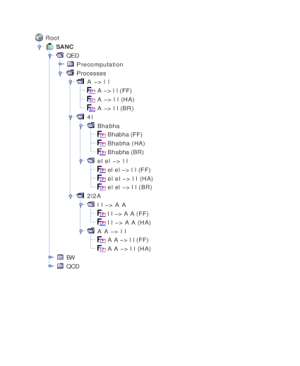
Figure 18: Available processes in QED part.

Both in QED and EW branches, modules BR compute analytically the contributions due to accompanying Bremsstrahlung. In this connection, present implementation of Bremsstrahlung into SANC is not homogeneous. As a rule, for all $1\to 2$ decays we have both Soft and Hard photon contributions. If only neutral particles are involved, for example $Z\to\nu\nu$, the module BR is not present in the tree. There is one exception: for $Z\to W^{+}W^{-}$ decay we have only one module FF, since it is unphysical and we implemented FF for future use as a building block for more complicated processes. As a rule, for $4f$ processes we also have both Soft and Hard photon Bremsstrahlung with exception of Bhabha process where we have only Soft contribution. For CC $2f_{1}\to 2f$ processes where we have realized quite involved calculations of Hard Bremsstrahlung with a possibility to impose simple cuts, see also [29]. For the tree body decays $t\to bl\nu$ we have implemented both Soft and Hard contributions. For $2f2b$ processes we had so far no BR and no s2n calculations.

This work is being started in version 1.10, where we have implemented FF and HA modules for three more $ffbb$ processes: $f_{1}\bar{f_{1}}\to ZZ$, $f_{1}\bar{f_{1}}\to ZH$ and $H\to f_{1}\bar{f_{1}}Z$. We recall, that $f_{1}$ stands for a massless fermion (its mass is retained only in the arguments of logs, if necessary). For the decay channel $H\to f_{1}\bar{f_{1}}Z$ and annihilation process $f_{1}\bar{f_{1}}\to ZH$ we have implemented (BR) modules and s2n calculations, see also [30] which contains an extensive presentation of numerical results.

$$\begin{array}[]{ccc}\vbox{\hbox{ \begin{picture}(100.0,100.0)(112.0,430.0)\includegraphics[width=227.62204pt,height=540.60236pt]{pro_ew_3leg_v110.ps} \end{picture}}}&&\vbox{\hbox{ \begin{picture}(100.0,100.0)(20.0,430.0)\includegraphics[width=227.62204pt,height=540.60236pt]{pro_ew_4leg_v110.ps} \end{picture}}}\end{array}$$

Figure 19: Available processes in EW part.

6 User Guide

6.1 Getting started

6.1.1 SANC installation

To work with SANC, one must install a SANC client on ones computer. The SANC client can be downloaded from the SANC project homepage http://sanc.jinr.ru or http://pcphsanc.cern.ch. On the homepage select Download, then download the client appropriate for your operational system (Linux, Windows), save it to your home directory and follow the instructions.

In Linux, opening the *.tgz file creates the directory /home/$<$user$>$/sanc_installer. Change to that directory, read the Readme and execute install.sh. SANC is then installed in /home/$<$user$>$/sanc_1.00.00. To start a SANC session, go to directory /home/$<$user$>$/sanc_1.00.00/bin and execute sanc.

In Windows, start sanc_installer.exe program and follow the instructions, restart computer. To start a SANC session, click SANC client icon.

6.1.2 SANC windows

At the beginning of a client session the main SANC window opens, see Fig. 20, with several toolbars and windows or fields:
$\bullet$ on top is the Menu bar with menus File, Edit, Build, Applications and View;
$\bullet$ underneath is a row of three Toolbars: File, Edit and Build
$\bullet$ underneath that on the left is the SANC tree field, and to the right of it the Editors List window; $\bullet$ underneath is the Output window and underneath that is the Console;
$\bullet$ below, at the bottom, lies the Status bar.
Other fields do arise in the course of the work.

The five menus have the options shown in Table 1. Menus with $\to$ have further extensions. For example, Toolbars has four options; they duplicate the File, Edit and Build toolbars, which are activated by default, and a latent option Memory. When the latter option is activated, two numbers are displayed: the first one is the current usage of the Java Virtual Machine (JVM) memory, and the second one is the total size of the JVM memory. All options can be unchecked in menu View $\to$ Toolbars $\to$.

Table 1: The SANC Menus and their options.

File	Edit	Build	Applications	View
Login …	Undo	Compile	Editor Form	Toolbars $\to$
Open Project …	Redo	Run S2N	Numeric Form	Projects
Mount Filesystem $\to$	Cut		Graphics Form	Editors List
Unmount Filesystem	Copy			Processes Table
Save	Paste			Console
Save All	Find			Output
Print … $\to$	Replace			Status Bar
Exit	Settings			ProgressBar
				Full Screen
				Look And Feel $\to$
				Suggestions

6.1.3 Login procedure

$\bullet$ To log in, click the Login icon (the first icon of the File toolbar). The Login panel opens with a choice of SANC servers: local, sanc.jinr.ru and pcphsanc.cern.ch; choose one of the latter ones (the local server is for PCs which have the server itself installed), then enter the login name guest and password guest.
$\bullet$ Click the Open Project icon (the second icon of the File toolbar). This opens the Open Project panel. There are two projects: Lessons and SANC. Select project SANC and press OK; then the SANC tree appears in the SANC tree field.

6.1.4 The SANC tree

The SANC tree has three options: QED, EW and QCD. Selection of one of these opens the next level of options: Precomputation and Processes.

Here we describe the sequence of steps for option EW $>$ Processes. The use of the Precomputation branch was described to an extent in Section 3.

The available processes are subdivided into 3legs and 4legs. The two branches of 3legs are 3b and b2f decays, and those of 4legs are 4f and 2f2b processes; here b and f denote any boson and fermion, respectively. For each of the latter two there is a branch for Neutral Current and a branch for Charged Current processes. The next branching is into the available processes of that class.

6.1.5 Naming conventions

In SANC we use naming conventions for fields (or particles) shown in Table 2 where N is the field index, and in the columns headed “name” we show the names used internally in SANC. All associated parameter symbols are derived from these names. Thus the mass, charge and weak isospin of the electron are denoted mel, qel and i3el, respectively, also the vector and axial vector coupling constants (vel, ael) and their sum (vpael) and difference (vmael).

Table 2: List of fields.

bosons			fermions									QCD
			1st generation			2nd generation			3rd generation
$N$	field	name	$N$	field	name	$N$	field	name	$N$	field	name	$N$	field	name
1	$A$	gm	11	$\nu_{e}$	en	15	$\nu_{\mu}$	mn	19	$\nu_{\tau}$	tn	23	g	gn
2	$Z$	z	12	$e^{-}$	el	16	$\mu^{-}$	mo	20	$\tau^{-}$	ta	24	$Y_{g}$	-
$\pm$3	$W^{\pm}$	w	13	$u$	up	17	$c$	ch	21	$t$	tp
4	$H$	h	14	$d$	dn	18	$s$	st	22	$b$	bt
5	$\phi^{0}$	-
$\pm$6	$\phi^{\pm}$	-
7	$X^{+}$	-
8	$X^{-}$	-
9	$Y_{\scriptscriptstyle{Z}}$	-
10	$Y_{\scriptscriptstyle{A}}$	-

Figure 20: Main SANC window

6.2 Benchmark case 1: $b\to ff$ decays

6.2.1 Semianalytical calculation

Consider the $Z\to b\bar{b}$ decay. First we open the relevant branch of the SANC tree:

EW $\to$ Processes $\to$ b2f $\to$ Z $\to$ ff

There are three FORM programs: (FF) Form Factor, (HA) Helicity Amplitudes, and (BR) Bremsstrahlung.

Select (FF) by a click with the right mouse button, this also pulls down a menu. On the menu left-click on Open. A Source Editor window opens with three tags: Form Editor, Fortran Editor, and Monte Carlo Editor. The first of these is activated by default and the FORM source code is displayed in the field.

The particle indices can be seen in the Console field; by default they are: typeB = 2 ($Z$ boson), typeU = 22 and typeD = 22 ($b$ quarks). To change the final state fermions, their particle numbers can be changed by editing them in the Console field and pressing Enter.

After choosing the process, open the Numeric Form panel from the Application menu. In this panel the particle masses and other relevant information are displayed.

Next the FORM code is compiled by clicking on the Compile button — the first icon in the Build toolbar (or by pressing the F7 function key). After compilation the FORM log file is shown in the Output field.

Clicking on the Run S2N button generates the FORTRAN code; the FORTRAN code can be seen in the Output field.
Repeat the sequence of steps for (HA) and (BR).

The progress of work can be monitored by activating the Processes Table (see Table 1).

The entire Output field is arranged in sheets with tags; for inspection any sheet can be brought to the forground by clicking on its tag.

Once the three FORM codes (FF), (HA) and (BR) have been compiled and tranfered to the FORTRAN codes one can get the numeric results by the following sequence of operations:

• open the FORTRAN editor sheet of the Editors List (belonging to the (FF) FORM code),

• open the Numeric Form panel from the Applications menu,

• press the Rehash button at the bottom of the Numeric Form panel, then the Compile button.

The answer appears in the Output field. It consists of a list of Input parameters and a set of results: $\Gamma(\mbox{born})$, the total width [TotalWidth] in Born approximation, $\Gamma(\mbox{born+virt+soft})$ and the total width, $\Gamma(\mbox{born+virt+soft+hard})$. Also shown is the parameter $\omega$, set to $10^{-10}\,\mbox{GeV}$ by default. This parameter defines the separation between soft and hard radiation. It can be modified in the corresponding box of the Numeric Form panel. Rerunning the program after changing the value of $\omega$ (using the sequence Rehash $>$ Compile) gives a result that differs only in the value of $\Gamma(\mbox{born+virt+soft})$. The born+virt+soft width is sensitive to parameter $\omega$ and can become unphysical (negative) for very small values of $\omega$. Increasing $\omega$ and rerunning gives positive values.

6.2.2 Monte Carlo calculation

The user can also carry out a Monte Carlo calculation generating various histograms: Photon Energy, Fermion Energy, Photon-Fermion Angular and Fermion-antiFermion Angular. To do this one must bring the Monte Carlo sheet of the Numeric Form to the foreground, check the boxes of the required histograms, then bring the MC sheet of the Editors List to the forground and rerun the program by clicking the Compile button. After a while the Histogram Form is displayed. This form has a menu bar; menu Option allows display of the histogram statistics. On the Monte Carlo sheet one can also select the random number generator, modify the number of MC events and the range of real photon energies $k_{0\,min}$ and $k_{0\,max}$, where $k_{0\,min}=\omega$ and $k_{0\,max}$ can be used as an experimental cut.
The Rehash button must be pressed after each change in the Numeric Form before clicking on the Compile button.

The results for the decay rates (in GeV) of the semianalytical calculation and of the Monte Carlo calculation for 100 000 events are summarised in Table 3. The numerical values are truncated to 6 significant figures.

Table 3: Benchmark Results for $\Gamma(Z\to b\bar{b})$ decay

		$\Gamma_{Born}$	$\Gamma_{Born+virt+soft}$	$\Gamma_{Total}$
SA		0.356948	0.336732	0.360224
MC	100 k			0.360229 $\pm$ 0.000721

6.3 Benchmark case 2: the process $2f\to 2f$

Consider the $4f$ CC process $f_{1}\bar{f}^{\prime}_{1}\to f\bar{f}^{\prime}$. Implemented are the processes ${u}\,\bar{d}\to\ell^{+}\,{\nu}_{\ell}$, its charge conjugate and the decay $t\to b\,\ell^{+}\,\nu_{\ell}$. For each process there are three FORM programs: (FF) Form Factor, (HA) Helicity Amplitudes, and (BR) Bremsstrahlung. Each of these in turn is opened, compiled and run as above in Section 6.2.

For process $u\,\bar{d}\to e^{+}\,{\nu}_{e}$ we have in the Console window the particle indices shown in Table 4.

Table 4: Assignment of particle numbers for process ${u}\,\bar{d}\to e^{+}\,{\nu}_{e}$

typeIU = 14	initial Up-type antiparticle ($\bar{d}$ quark)
typeID = 13	initial Down-type particle ($u$ quark)
typeFU = 12	final Up-type antiparticle (positron)
typeFD = 11	final Down-type particle (neutrino)

These can be changed to typeIU = 13, typeID = 14, typeFU = 11 and typeFD = 12 for process $\bar{u}\,{d}\to e^{-}\,\bar{\nu}_{e}$ by editing the particle numbers as explained above.

Next bring the Fortran Editor sheet of the Editors List and the Numeric Form panel to the foreground. Shown on the Numeric Parameter sheet are the particle masses in GeV/$c^{2}$ and the CMS energy in GeV, also the cosine of the CMS angle between the incident and outgoing particle momenta.

Click on the Rehash button at the bottom of the Numeric Form panel: the main module of FORTRAN code appears in the Fortran Editor sheet of the Editors List. Then click on Compile. The final answer appears in the Output field. It consists of the parameters used ($\alpha$, $G_{F}$, particle masses, the ’t Hooft scale $\mu$ and the Mandelstam variables), and the resulting differential cross sections $d\,\sigma/d\,\cos\,\theta$ in picobarns in the Born approximation and Born+one-loop. The results for the default parameters and for several scattering angles are summarised in Table 5. The numerical values are truncated to 6 figures.

Table 5: CMS differential cross sections in pb for $u\bar{d}\to e^{+}\nu_{e}$

		$\sqrt{s}$ GeV
$\cos\theta$		40	80	120
-0.9	Born	3.58202	10818.4	12.0561
	Born + one-loop	3.53427	9990.97	28.1226
-0.5	Born	2.23256	6742.78	7.51423
	Born + one-loop	2.18961	6226.00	12.8563
0.0	Born	0.99225	2996.79	3.33966
	Born + one-loop	0.97192	2769.11	5.12160
0.5	Born	0.24806	749.198	0.83491
	Born + one-loop	0.24453	695.224	1.47999
0.9	Born	0.00992	29.9679	0.03339
	Born + one-loop	0.01072	30.2878	0.09277

Here the one-loop corrections are purely weak and QED corrections comprise one-loop virtual QED corrections and soft and hard radiations.

The Born+one-loop cross section is insensitive to the ’t Hooft scale parameter $\mu$ which cancels between one-loop electroweak and the QED part of virtual corrections.

Input parameters can be changed by editing the appropriate field of the Numeric Form panel and pressing the Rehash button. Again the Rehash button must be pressed before pressing Compile.

In the NC sector there are many more processes. Here $f_{1}$ is a massless fermion of the first generation or any neutrino, and $f$ is any fermion. All procedures described above for the CC processes apply also in this case.

Monte Carlo calculations are not yet implemented for $2\to 2$ processes.

Acknowledgments

The authors are very much indebted to G. Passarino for critical reading of the manuscript and useful comments. We are grateful to S. Jadach, W. Placzek, F. Tkachov, B. Ward, and Z. Was for numerous discussions. We thank V. Kolesnikov and E. Uglov for managing and supporting the SANC computer system.

References

- [1] D. Bardin and G. Passarino, The standard model in the making: Precision study of the electroweak interactions. Clarendon, 1999. Oxford, UK.
- [2] D. Bardin, G. Passarino, L. Kalinovskaya, P. Christova, A. Andonov, S. Bondarenko, and G. Nanava, Project CalcPHEP: Calculus for precision high energy physics, Proceedings of the International Workshop on Computer Algebra and its Application to Physics, CAAP-2001, Dubna 2001. Edited by V.P. Gerdt.
- [3] D. Bardin et al., Comput. Phys. Commun. 133 (2001) 229–395.
- [4] A. Arbuzov et al., Comput. Phys. Commun. 94 (1996) 128–184.
- [5] D. Bardin, J. Blumlein, P. Christova, and L. Kalinovskaya, Nucl. Phys. B506 (1997) 295–328.
- [6] D. Bardin and L. Kalinovskaya, QED corrections for polarized elastic scattering, hep-ph/9712310.
- [7] J. A. M. Vermaseren, New features of FORM, math-ph/0010025.
- [8] D. Bardin, P. Christova, L. Kalinovskaya, and G. Passarino, Eur. Phys. J. C22 (2001) 99–104.
- [9] A. Andonov et al., Phys. Part. Nucl. 34 (2003) 577–618.
- [10] A. Arbuzov, D. Bardin, and L. Kalinovskaya, Radiative corrections to neutrino deep inelastic scattering revisited, JHEP 06 (2005) 078. hep-ph/0407203.
- [11] A. Andonov et al., Nucl. Instrum. Meth. A502 (2003) 576–577.
- [12] L. V. Kalinovskaya, Nucl. Instrum. Meth. A502 (2003) 581–582.
- [13] P. Christova, Nucl. Instrum. Meth. A502 (2003) 578–580.
- [14] G. Nanava, Nucl. Instrum. Meth. A502 (2003) 583–585.
- [15] A. Andonov et al., Project SANC (former CalcPHEP): Support of analytic and numeric calculations for experiments at colliders, Proceedings of 31st International Conference on High Energy Physics (ICHEP 2002), Amsterdam, The Netherlands, 24-31 Jul 2002. Amsterdam 2002, ICHEP pp.825–827, hep-ph/0209297.
- [16] D. Bardin, P. Christova, and L. Kalinovskaya, Nucl. Phys. Proc. Suppl. 116 (2003) 48–52.
- [17] D. Bardin and L. Kalinovskaya, Present Status of CalcPHEP Project and Update of one-loop corrections for , first run of CalcPHEP system, 2002, ECFA Study Workshop, Saint-Malo, France.
- [18] D. Bardin and L. Kalinovskaya, Project SANC: Ideas and Realization and SANC: Procecesses, 2003, CERN Workshop on Monte Carlo generators for LHC, Geneva.
- [19] D. Bardin, L. Kalinovskaya, and A. Arbuzov, Present Status of the Project SANC and SANC: Processes and SANC and Deep Inelastic Neutrino Scattering, 2003, ECFA Study Workshop, Montpelier, France.
- [20] A. Arbuzov, D. Bardin, and L. Kalinovskaya, Electroweak radiative corrections to neutrino DIS, talk presented at Linear Collider Workshop in Paris, 19-23 April 2004, to appear in Proceedings.
- [21] R. Vega and J. Wudka, Phys. Rev. D53 (1996) 5286–5292.
- [22] R. Kleiss and W. J. Stirling, Nucl. Phys. B262 (1985) 235–262.
- [23] T. Hahn, Comput. Phys. Commun. 140 (2001) 418–4570.
- [24] J. Fleischer et al., One-loop corrections to the process including hard bremsstrahlung, hep-ph/0203220.
- [25] J. Fleischer et al., Complete electroweak one-loop radiative corrections to top-pair production at TESLA – a comparison, LC-TH-2002-002, hep-ph/0202109.
- [26] A. Andonov, S. Jadach, G. Nanava, and Z. Was, Acta Phys. Polon. B34 (2003) 2665–2672.
- [27] G. Nanava and Z. Was, Acta Phys. Polon. B34 (2003) 4561–4570.
- [28] A. Andonov et al. A second part of the SANC description, in preparation.
- [29] A. Arbuzov et al., One-loop corrections to the Drell–Yan in SANC (I). The Charged Current case. Jun 2005. 11pp. hep-ph/0506110.
- [30] D. Bardin et al., SANCnews: Sector . Jun 2005. 16pp. hep-ph/0506120.