Abstract

We evaluate ${\cal O}(\alpha_{b}\alpha_{s})$ corrections in the Higgs boson sector of the ${\cal CP}$-conserving MSSM, generalising the known result in the literature to arbitrary values of $\tan\beta$. A detailed analysis of the renormalisation in the bottom/scalar bottom sector is performed. Concerning the lightest MSSM Higgs boson mass, we find relatively small corrections for positive $\mu$, while for $\mu<0$ the genuine two-loop ${\cal O}(\alpha_{b}\alpha_{s})$ corrections can amount up to 3 GeV. Different renormalisation schemes are applied and numerically compared. It is demonstrated that some care has to be taken in choosing an appropriate renormalisation prescription in order to avoid artificially large corrections. The residual dependence on the renormalisation scale is investigated, and the remaining theoretical uncertainties from unknown higher-order corrections in this sector are discussed for different regions of the MSSM parameter space.

1 Introduction

A crucial prediction of the Minimal Supersymmetric Standard Model (MSSM) [1] is the existence of at least one light Higgs boson. The search for this particle is one of the main goals at the present and the next generation of colliders. Direct searches at LEP have already ruled out a considerable fraction of the MSSM parameter space [2, 3], and the forthcoming high-energy experiments at the Tevatron, the LHC, and the International Linear Collider (ILC) will either discover a light Higgs boson or rule out Supersymmetry (SUSY) as a viable theory for physics at the weak scale. Furthermore, if one or more Higgs bosons are discovered, bounds on their masses and couplings will be set at the LHC [4, 5, 6]. Eventually the masses and couplings will be determined with high accuracy at the ILC [7, 8, 9]. Thus, a precise knowledge of the dependence of masses and mixing angles in the MSSM Higgs sector on the relevant supersymmetric parameters is of utmost importance to reliably compare the predictions of the MSSM with the (present and future) experimental results.

The status of the available results for the higher-order contributions to the neutral ${\cal CP}$-even MSSM Higgs boson masses can be summarised as follows. For the one-loop part, the complete result within the MSSM is known [10, 11, 12, 13]. The dominant one-loop contribution is the ${\cal O}(\alpha_{t})$ term due to top and stop loops ($\alpha_{t}\equiv h_{t}^{2}/(4\pi)$, $h_{t}$ being the superpotential top coupling). Corrections from the bottom/sbottom sector can also give large effects, in particular for large values of $\tan\beta$, the ratio of the two vacuum expectation values, $\tan\beta=v_{2}/v_{1}$. The computation of two-loop corrections is also quite advanced. It has now reached a stage such that all the presumably dominant contributions are known. They include the strong corrections, usually indicated as ${\cal O}(\alpha_{t}\alpha_{s})$, and Yukawa corrections, ${\cal O}(\alpha_{t}^{2})$, to the dominant one-loop ${\cal O}(\alpha_{t})$ term, as well as the strong corrections to the bottom/sbottom one-loop ${\cal O}(\alpha_{b})$ term ($\alpha_{b}\equiv h_{b}^{2}/(4\pi)$), i.e. the ${\cal O}(\alpha_{b}\alpha_{s})$ contribution, derived in the limit $\tan\beta\to\infty$. Presently, the ${\cal O}(\alpha_{t}\alpha_{s})$ [14, 15, 16, 17, 18, 19, 20, 21, 22, 23], ${\cal O}(\alpha_{t}^{2})$ [14, 15, 24, 25] and the ${\cal O}(\alpha_{b}\alpha_{s})$ [26] contributions to the self-energies are known for vanishing external momenta. Most recently also the corrections ${\cal O}(\alpha_{t}\alpha_{b})$ and ${\cal O}(\alpha_{b}^{2})$ [27], a “full” two-loop effective potential calculation [28] and an evaluation of the leading two-loop momentum dependent effects [29] have become available. In the (s)bottom corrections the all-order resummation of the $\tan\beta$-enhanced terms, ${\cal O}(\alpha_{b}(\alpha_{s}\tan\beta)^{n})$, is also performed [30, 31]. Reviews with further references can be found in Refs. [32, 33, 34].

The $b/\tilde{b}$ sector has attracted considerable attention in the last years, since its corrections to the MSSM Higgs boson sector have been found to be large in certain parts of the MSSM parameter space, possibly even exceeding the size of the top/stop corrections. This can happen especially for large values of $\tan\beta$ and the supersymmetric Higgs mass parameter $\mu$. For illustration, we show in Fig. 1 the shift in the lightest ${\cal CP}$-even Higgs boson mass, $\Delta M_{h}$, arising from the $b/\tilde{b}$ sector at the one-loop level (all two-loop corrections are omitted here) as a function of the bottom-quark mass for large $\tan\beta$ and $|\mu|$. The bottom-quark mass in this plot is understood to be an effective mass that includes higher-order effects (see the discussion in Sect. 3). The figure demonstrates that corrections from the $b/\tilde{b}$ sector can get large if the effective bottom mass is bigger than about 3 GeV.

Figure 1: The shift in the lightest ${\cal CP}$-even Higgs-boson mass from the one-loop corrections in the $b/\tilde{b}$ sector is shown as a function of the (effective) bottom-quark mass for $\mu=\pm 1000\,\,{\rm GeV}$, $\tan\beta=50$, $M_{\text{SUSY}}=600\,\,{\rm GeV}$, $A_{t}=A_{b}=500\,\,{\rm GeV}$, $M_{A}=700\,\,{\rm GeV}$.

The possibly large size of the corrections from the $b/\tilde{b}$ sector makes it desirable to investigate the corresponding two-loop corrections and thus to analyse the renormalisation in this sector. An inconvenient choice could give rise to artificially large corrections, whereas a convenient scheme absorbs the dominant contributions into the one-loop result such that higher-order corrections remain small. The comparison of different schemes (where no artificially enhanced corrections appear) gives an indication of the possible size of missing higher-order terms of ${\cal O}(\alpha_{b}\alpha_{s}^{2})$.

In this paper we derive the result for the ${\cal O}(\alpha_{b}\alpha_{s})$ corrections in various renormalisation schemes. The relations between the different parameters in these schemes are worked out in detail. The absorption of leading higher-order contributions into an effective bottom-quark mass is discussed. We perform a numerical analysis of the various schemes and compare our results with a previous evaluation of the ${\cal O}(\alpha_{b}\alpha_{s})$ corrections carried out in the limit where $\tan\beta$ is infinitely large [26]. We discuss the dependence of our result on the renormalisation scale and provide an estimate of the remaining theoretical uncertainties in this sector.

The paper is organised as follows: in Sect. 2 we briefly review the MSSM Higgs boson sector, outline the corresponding renormalisation at the two-loop level, and describe the evaluation of the diagrams of ${\cal O}(\alpha_{b}\alpha_{s})$. Sect. 3 contains a detailed description of the renormalisation of the scalar top and scalar bottom sector, which is explicitly carried out in four different renormalisation schemes for the latter. The numerical analysis of the ${\cal O}(\alpha_{b}\alpha_{s})$ corrections, the comparison of the different schemes, the investigation of the renormalisation scale, and the comparison with the previous result are performed in Sect. 4. The conclusions can be found in Sect. 5.

2 The Higgs sector at higher orders

We recall that the Higgs sector of the MSSM [35] comprises two neutral ${\cal CP}$-even Higgs bosons, $h$ and $H$ ($m_{h}<m_{H}$), the ${\cal CP}$-odd $A$ boson, and two charged Higgs bosons, $H^{\pm}$. At the tree-level, the masses $m_{h,{\rm tree}}$ and $m_{H,{\rm tree}}$ can be calculated in terms of $M_{Z}$, $M_{A}$ and $\tan\beta$ from the mass matrix for the neutral ${\cal CP}$-even Higgs components (denoted by $\phi$)

$${\cal M}_{\phi} = \left(\begin{array}[]{cc}M_{A}^{2}\sin^{2}\beta\hskip 2.84526pt+M_{Z}^{2}\cos^{2}\beta&-(M_{A}^{2}+M_{Z}^{2})\sin\beta\cos\beta\\ -(M_{A}^{2}+M_{Z}^{2})\sin\beta\cos\beta&M_{A}^{2}\cos^{2}\beta\hskip 2.84526pt+M_{Z}^{2}\sin^{2}\beta\end{array}\right)$$ (3)

by diagonalization,

$$\left(\begin{array}[]{cc}m_{H,{\rm tree}}^{2}&0\\ 0&m_{h,{\rm tree}}^{2}\end{array}\right) = {\cal U}_{\phi}\,{\cal M}_{\phi}\,{\cal U}_{\phi}^{\dagger}~{},\qquad{\cal U}_{\phi}=\left(\begin{array}[]{cc}\cos\alpha&\sin\alpha\\ -\sin\alpha&\cos\alpha\end{array}\right)\,,$$ (8)

with the angle $\alpha$ determined by

$$\tan 2\alpha=\tan 2\beta\,\frac{M_{A}^{2}+M_{Z}^{2}}{M_{A}^{2}-M_{Z}^{2}},\quad-\frac{\pi}{2}<\alpha<0.$$ (9)

In the Feynman-diagrammatic (FD) approach, the higher-order corrected Higgs boson masses, $M_{h}$ and $M_{H}$, are derived as the poles of the $h,H$-propagator matrix, i.e. by solving the equation

$$\left[p^{2}-m_{h,{\rm tree}}^{2}+\hat{\Sigma}_{hh}(p^{2})\right]\left[p^{2}-m_{H,{\rm tree}}^{2}+\hat{\Sigma}_{HH}(p^{2})\right]-\left[\hat{\Sigma}_{hH}(p^{2})\right]^{2}=0\,.$$ (10)

The renormalised self-energies

$$\hat{\Sigma}(p^{2})=\left(\begin{array}[]{cc}\hat{\Sigma}_{HH}(p^{2})&\hat{\Sigma}_{hH}(p^{2})\\[1.99997pt] \hat{\Sigma}_{hH}(p^{2})&\hat{\Sigma}_{hh}(p^{2})\end{array}\right)$$ (11)

can be expanded according to the one-, two-, …loop-order contributions,

$$\hat{\Sigma}(p^{2})=\hat{\Sigma}^{(1)}(p^{2})+\hat{\Sigma}^{(2)}(p^{2})+\cdots~{}.$$ (12)

The dominant one-loop contributions to the Higgs boson self-energies (and thus to the Higgs boson masses) from the $b/\tilde{b}$ sector are of ${\cal O}(\alpha_{b})$ and arise from the Yukawa part of the theory (neglecting the gauge couplings) evaluated at $p^{2}=0$. This has been verified by comparison with the full one-loop result from the $b/\tilde{b}$ sector. Hence, the leading two-loop corrections from the $b/\tilde{b}$ sector are the ${\cal O}(\alpha_{s})$ corrections to those dominant one-loop contributions; they are obtained in the same limit, i.e. for zero external momentum and neglecting the gauge couplings (the same approximations have been made in Ref. [26]). This approach is analogous to the way the leading one- and two-loop contributions in the top/stop sector have been obtained, see e.g. Ref. [19].

The renormalisation of the Higgs-boson mass matrix for the ${\cal O}(\alpha_{b}\alpha_{s})$ corrections under consideration follows the description for the ${\cal O}(\alpha_{t}\alpha_{s})$ terms given in Ref. [19]. Renormalisation can be performed by adding the appropriate counterterms,

$${\cal M}_{\phi} \to{\cal M}_{\phi}+\delta{\cal M}^{(1)}_{\phi}+\delta{\cal M}^{(2)}_{\phi}+\cdots\,,$$ (13)

where $\delta{\cal M}^{(i)}_{\phi}$ denotes the ith-loop counterterm matrix consisting of the counterterms to the parameters in the tree-level mass matrix (3). Field renormalisation is not needed for the leading ${\cal O}(\alpha_{b}\alpha_{s})$ corrections. The renormalised two-loop Higgs boson self-energies with the leading contributions of ${\cal O}(\alpha_{b}\alpha_{s})$ are thus given by

$$\hat{\Sigma}^{(2)}(0) =\Sigma^{(2)}(0)-{\cal U}_{\phi}\delta{\cal M}_{\phi}^{(2)}{\cal U}^{\dagger}_{\phi}~{}.$$ (14)

The counterterm matrix in (14) is composed of the counterterms for the $A$-boson mass and for the tadpoles $t_{h,H}$ (with $s_{\mathrm{w}}\equiv\sin\theta_{W}$, $c_{\mathrm{w}}=\cos\theta_{W}$),

$$\delta{\cal M}_{\phi}^{(2)} =\begin{pmatrix}\sin^{2}\beta&-\sin\beta\cos\beta\\ -\sin\beta\cos\beta&\cos^{2}\beta\end{pmatrix}\delta M_{A}^{2\,(2)}$$

$$\quad\ +\frac{e}{2M_{Z}c_{\mathrm{w}}s_{\mathrm{w}}}\begin{pmatrix}-\cos\beta(1+\sin^{2}\beta)&-\sin^{3}\beta\\ -\sin^{3}\beta&\cos\beta\sin^{2}\beta\end{pmatrix}(\cos\alpha\,\delta t_{H}^{(2)}-\sin\alpha\,\delta t_{h}^{(2)})$$

$$\quad\ +\frac{e}{2M_{Z}c_{\mathrm{w}}s_{\mathrm{w}}}\begin{pmatrix}\cos^{2}\beta\sin\beta&-\cos^{3}\beta\\ -\cos^{3}\beta&-(1+\cos^{2}\beta)\sin\beta\end{pmatrix}(\sin\alpha\,\delta t_{H}^{(2)}+\cos\alpha\,\delta t_{h}^{(2)})\,.$$ (15)

The counterterms are determined by the following conditions:

• On-shell renormalisation of the $A$-boson mass, formulated in the approximation of vanishing external momentum, determines the two-loop $A$-mass counterterm $\delta M_{A}^{2\,(2)}$ according to

  $$\delta M_{A}^{2\,(2)}=\Sigma^{(2)}_{AA}(0)\,.$$ (16)

• Tadpole renormalisation determines the tadpole counterterms by the requirements

  $$\delta t_{H}^{(2)} =-t_{H}^{(2)}\,,\quad\delta t_{h}^{(2)} =-t_{h}^{(2)}\,,$$ (17)

  which means that the minimum of the Higgs potential is not shifted.

Figure 2: Generic two-loop diagrams for the Higgs-boson self-energies ($\phi=h,H,A$; $\;i,j,k,l=1,2$).

Figure 3: Generic two-loop diagrams for the Higgs tadpoles ($\phi=h,H$; $\;i,j,k=1,2$).

Figure 4: Generic one-loop diagrams with counterterm insertion for the Higgs-boson self-energies ($\phi=h,H,A$), $\;i,j,k=1,2$).

Figure 5: Generic one-loop diagrams with counterterm insertion for the Higgs tadpoles ($\phi=h,H$, $\;i,j=1,2$).

The genuine two-loop Feynman diagrams to be evaluated for the Higgs boson self-energies and the tadpoles are shown Fig. 2 and Fig. 3. The diagrams with subloop renormalisation are depicted in Fig. 4 and Fig. 5. The counterterms for the insertions, where different renormalisation schemes will be investigated, are specified in the next section.

The diagrams and the corresponding amplitudes have been generated with the package FeynArts [36, 37]. The further evaluation has been done using the program TwoCalc [38]. The resulting expressions are given in terms of the one-loop functions $A_{0}$ and $B_{0}$ [39], and the two-loop vacuum integrals [40].

3 Renormalisation of the quark/squark sector

Since the two-loop self-energy is considered at $\mathcal{O}(\alpha_{\{t,\,b\}}\alpha_{s})$ it is sufficient to determine the counterterms induced by the strong interaction only.

The squark-mass terms of the Lagrangian, for a given species of squarks $\tilde{q}$, can be written as the bilinear expression

$${\cal L}_{\tilde{q}\text{-mass}} =-\begin{pmatrix}\tilde{q}_{L}^{\dagger},\tilde{q}_{R}^{\dagger}\end{pmatrix}{\cal M}_{\tilde{q}}\begin{pmatrix}\tilde{q}_{L}\\ \tilde{q}_{R}\end{pmatrix},$$ (18)

with ${\cal M}_{\tilde{q}}$ as the squark-mass matrix squared,

$${\cal M}_{\tilde{q}}=\begin{pmatrix}M_{L}^{2}+m_{q}^{2}+M_{Z}^{2}c_{2\beta}(T_{q}^{3}-Q_{q}s_{\mathrm{w}}^{2})&m_{q}(A_{q}-\mu\kappa)\\[1.99997pt] m_{q}(A_{q}-\mu\kappa)&M_{\tilde{q}_{R}}^{2}+m_{q}^{2}+M_{Z}^{2}c_{2\beta}Q_{q}s_{\mathrm{w}}^{2}\end{pmatrix},$$ (19)

where the quantities $M_{L}^{2}$, $M_{\tilde{q}_{R}}^{2}$, $A_{q}$ are soft-breaking parameters, and $\mu$ is the supersymmetric Higgs mass parameter. Since we are dealing in this paper with a ${\cal CP}$-conserving Higgs sector, these parameters are treated as real. As an abbreviation, $c_{2\beta}\equiv\cos(2\beta)$ is introduced; $\kappa$ is defined as $\kappa=\cot\beta$ for up-type squarks and $\kappa=\tan\beta$ for down-type squarks. $m_{q}$, $Q_{q}$, and $T_{q}^{3}$ are mass, charge, and isospin of the quark $q$.

The mass matrix (19) can be diagonalised by a unitary transformation, which in our case of real parameters involves a mixing angle $\theta\kern-1.49994pt_{\tilde{q}}$,

$$\begin{pmatrix}\tilde{q}_{1}\\ \tilde{q}_{2}\end{pmatrix}={\cal U}_{\tilde{q}}\begin{pmatrix}\tilde{q}_{L}\\ \tilde{q}_{R}\end{pmatrix}\,,\qquad{\cal U}_{\tilde{q}}=\begin{pmatrix}U_{\tilde{q}_{11}}&U_{\tilde{q}_{12}}\\ U_{\tilde{q}_{21}}&U_{\tilde{q}_{22}}\end{pmatrix}=\begin{pmatrix}\cos\theta\kern-1.49994pt_{\tilde{q}}&\sin\theta\kern-1.49994pt_{\tilde{q}}\\ -\sin\theta\kern-1.49994pt_{\tilde{q}}&\cos\theta\kern-1.49994pt_{\tilde{q}}\end{pmatrix}\,.$$ (20)

In the $(\tilde{q}_{1},\tilde{q}_{2})$-basis, the squared-mass matrix is diagonal,

$${\cal D}_{\tilde{q}} ={\cal U}_{\tilde{q}}{{\cal M}}_{\tilde{q}}{{\cal U}}_{\tilde{q}}^{\dagger}=\begin{pmatrix}m_{\tilde{q}_{1}}^{2}&0\\ 0&m_{\tilde{q}_{2}}^{2}\end{pmatrix}\,,$$ (21)

with the eigenvalues $m_{\tilde{q}_{1}}^{2}$ and $m_{\tilde{q}_{2}}^{2}$ given by

$$m_{\tilde{q}_{1,2}}^{2}=\frac{1}{2}(M_{L}^{2}+M_{\tilde{q}_{R}}^{2})+m_{q}^{2}+\frac{1}{2}T_{q}^{3}M_{Z}^{2}c_{2\beta}\pm\frac{1}{2}\frac{M_{L}^{2}-M_{\tilde{q}_{R}}^{2}+M_{Z}^{2}c_{2\beta}(T_{q}^{3}-2Q_{q}s_{\mathrm{w}}^{2})}{|M_{L}^{2}-M_{\tilde{q}_{R}}^{2}+M_{Z}^{2}c_{2\beta}(T_{q}^{3}-2Q_{q}s_{\mathrm{w}}^{2})|}$$

$$\qquad\ \quad\times\sqrt{\bigl{[}M_{L}^{2}-M_{\tilde{q}_{R}}^{2}+M_{Z}^{2}c_{2\beta}(T_{q}^{3}-2Q_{q}s_{\mathrm{w}}^{2})\bigr{]}^{2}+4m_{q}^{2}(A_{q}-{\mu}\kappa)^{2}}\;.$$ (22)

The squark-mass matrix can now be expressed in terms of the two mass eigenvalues and the mixing angle, yielding

$${\cal M}_{\tilde{q}}=\left(\begin{array}[]{cc}\cos^{2}\theta\kern-1.49994pt_{\tilde{q}}\;m_{\tilde{q}_{1}}^{2}+\sin^{2}\theta\kern-1.49994pt_{\tilde{q}}\;m_{\tilde{q}_{2}}^{2}&\sin\theta\kern-1.49994pt_{\tilde{q}}\cos\theta\kern-1.49994pt_{\tilde{q}}\,(m_{\tilde{q}_{1}}^{2}-m_{\tilde{q}_{2}}^{2})\\[3.99994pt] \sin\theta\kern-1.49994pt_{\tilde{q}}\cos\theta\kern-1.49994pt_{\tilde{q}}\,(m_{\tilde{q}_{1}}^{2}-m_{\tilde{q}_{2}}^{2})&\sin^{2}\theta\kern-1.49994pt_{\tilde{q}}\;m_{\tilde{q}_{1}}^{2}+\cos^{2}\theta\kern-1.49994pt_{\tilde{q}}\;m_{\tilde{q}_{2}}^{2}\end{array}\right)~{}.$$ (23)

3.1 Renormalisation of the top and scalar top sector

The $(t,\tilde{t})$ sector contains four independent parameters: the top-quark mass $m_{t}$, the stop masses $m_{\tilde{t}_{1}}$ and $m_{\tilde{t}_{2}}$, and either the squark mixing angle $\theta_{\tilde{t}}$ or, equivalently, the trilinear coupling $A_{t}$. Accordingly, the renormalisation of this sector is performed by introducing four counterterms that are determined by four independent renormalisation conditions.

The following renormalisation conditions are imposed (the procedure is equivalent to that of Ref. [41], although there no reference is made to the mixing angle).

• On-shell renormalisation of the top-quark mass yields the top mass counterterm,

  $$\delta m_{t}=\frac{1}{2}m_{t}\bigl{[}\mathop{\rm Re}\Sigma_{{t}_{L}}(m_{t}^{2})+\mathop{\rm Re}\Sigma_{{t}_{R}}(m_{t}^{2})+2\mathop{\rm Re}\Sigma_{{t}_{S}}(m_{t}^{2})\bigr{]}\;,$$ (24)

  with the scalar coefficients of the unrenormalised top-quark self-energy, $\Sigma_{t}(p)$, in the Lorentz decomposition

  $$\Sigma_{t}(p) =\makebox[0.86108pt][l]{$p$}/\omega_{-}\Sigma_{{t}_{L}}(p^{2})+\makebox[0.86108pt][l]{$p$}/\omega_{+}\Sigma_{{t}_{R}}(p^{2})+m_{t}\Sigma_{{t}_{S}}(p^{2})\;.$$ (25)

• On-shell renormalisation of the stop masses determines the mass counterterms

  $$\delta m_{\tilde{t}_{1}}^{2}=\mathop{\rm Re}\Sigma_{\tilde{t}_{11}}(m_{{\tilde{t}}_{1}}^{2})\,,\quad\delta m_{\tilde{t}_{2}}^{2}=\mathop{\rm Re}\Sigma_{\tilde{t}_{22}}(m_{{\tilde{t}}_{2}}^{2})\;,$$ (26)

  in terms of the diagonal squark self-energies.

• The counterterm for the mixing angle, $\theta_{\tilde{t}}$, (entering (23)) is fixed in the following way,

  $$\delta\theta_{\tilde{t}}=\frac{\mathop{\rm Re}\Sigma_{\tilde{t}_{12}}(m_{{\tilde{t}}_{1}}^{2})+\mathop{\rm Re}\Sigma_{\tilde{t}_{12}}(m_{{\tilde{t}}_{2}}^{2})}{2(m_{\tilde{t}_{1}}^{2}-m_{\tilde{t}_{2}}^{2})}\;,$$ (27)

  involving the non-diagonal squark self-energy. (This is a convenient choice for the treatment of ${\cal O}(\alpha_{s})$ corrections. If electroweak contributions were included, a manifestly gauge-independent definition would be more appropriate.)

In the renormalised vertices with squark and Higgs fields, the counterterm of the trilinear coupling $A_{t}$ appears. Having already specified $\delta\theta_{\tilde{t}}$, the $A_{t}$ counterterm cannot be defined independently but follows from the relation

$$\sin 2\theta_{\tilde{t}}=\frac{2m_{t}(A_{t}-\mu\cot\beta)}{m_{\tilde{t}_{1}}^{2}-m_{\tilde{t}_{2}}^{2}}\,,$$ (28)

yielding

$$\delta A_{t} =\frac{1}{m_{t}}\Bigl{[}\frac{1}{2}\sin 2\theta_{\tilde{t}}\bigl{(}\delta m_{\tilde{t}_{1}}^{2}-\delta m_{\tilde{t}_{2}}^{2}\bigr{)}+\cos 2\theta_{\tilde{t}}(m_{\tilde{t}_{1}}^{2}-m_{\tilde{t}_{2}}^{2})\,\delta\theta_{\tilde{t}}$$

$$\quad\ \quad\ -\frac{1}{2m_{t}}\sin 2\theta_{\tilde{t}}(m_{\tilde{t}_{1}}^{2}-m_{\tilde{t}_{2}}^{2})\,\delta m_{t}\Bigr{]}~{}.$$ (29)

This relation is valid at ${\cal O}(\alpha_{s})$ since both $\mu$ and $\tan\beta$ do not receive one-loop contributions from the strong interaction.

3.2 Renormalisation of the bottom and scalar bottom sector

Because of SU(2)-invariance the soft-breaking parameters for the left-handed up- and down-type squarks are identical, and thus the squark masses of a given generation are not independent. The stop and sbottom masses are connected via the relation

$$\cos^{2}\theta_{\tilde{b}}m_{\tilde{b}_{1}}^{2}+\sin^{2}\theta_{\tilde{b}}m_{\tilde{b}_{2}}^{2}=\cos^{2}\theta_{\tilde{t}}m_{\tilde{t}_{1}}^{2}+\sin^{2}\theta_{\tilde{t}}m_{\tilde{t}_{2}}^{2}+m_{b}^{2}-m_{t}^{2}-M_{W}^{2}\cos(2\beta)~{},$$ (30)

with the entries of the rotation matrix in (20). Since the stop masses have already been renormalised on-shell, only one of the sbottom mass counterterms can be determined independently. In the following, the $\tilde{b}_{2}$ mass is chosen as the pole mass yielding the counterterm from an on-shell renormalisation condition, i.e.

$$\delta m_{\tilde{b}_{2}}^{2} =\mathop{\rm Re}\Sigma_{\tilde{b}_{22}}(m_{\tilde{b}_{2}}^{2})\;,$$ (31)

whereas the counterterm for $m_{\tilde{b}_{1}}$ is determined as a combination of other counterterms, according to

$$\delta m_{\tilde{b}_{1}}^{2} =\frac{1}{\cos^{2}\theta_{\tilde{b}}}\Bigl{(}\cos^{2}\theta_{\tilde{t}}\delta m_{\tilde{t}_{1}}^{2}+\sin^{2}\theta_{\tilde{t}}\delta m_{\tilde{t}_{2}}^{2}-\sin^{2}\theta_{\tilde{b}}\delta m_{\tilde{b}_{2}}^{2}-\sin 2\theta_{\tilde{t}}(m_{\tilde{t}_{1}}^{2}-m_{\tilde{t}_{2}}^{2})\delta\theta_{\tilde{t}}$$

$$\quad+\sin 2\theta_{\tilde{b}}(m_{\tilde{b}_{1}}^{2}-m_{\tilde{b}_{2}}^{2})\delta\theta_{\tilde{b}}-2m_{t}\,\delta m_{t}+2m_{b}\,\delta m_{b}\Bigr{)}~{}.$$ (32)

Accordingly, the numerical value of $m_{\tilde{b}_{1}}$ does not correspond to the pole mass. The pole mass can be obtained from $m_{\tilde{b}_{1}}$ via a finite shift of $\mathcal{O}(\alpha_{s})$ (see e.g. Ref. [42]).

There are three more parameters with counterterms to be determined: the $b$-quark mass $m_{b}$, the mixing angle $\theta_{\tilde{b}}$, and the trilinear coupling $A_{b}$. They are connected via

$$\sin 2\theta_{\tilde{b}}=\frac{2m_{b}(A_{b}-\mu\tan\beta)}{m_{\tilde{b}_{1}}^{2}-m_{\tilde{b}_{2}}^{2}}\,,$$ (33)

which reads in terms of counterterms

$$2\cos 2\theta_{\tilde{b}}\;\delta\theta_{\tilde{b}} =\sin 2\theta_{\tilde{b}}\frac{\delta m_{b}}{m_{b}}+\frac{2m_{b}\,\delta A_{b}}{m_{\tilde{b}_{1}}^{2}-m_{\tilde{b}_{2}}^{2}}-\sin 2\theta_{\tilde{b}}\frac{\delta m_{\tilde{b}_{1}}^{2}-\delta m_{\tilde{b}_{2}}^{2}}{m_{\tilde{b}_{1}}^{2}-m_{\tilde{b}_{2}}^{2}}~{}.$$ (34)

Only two of the three counterterms, $\delta m_{b}$, $\delta\theta_{\tilde{b}}$, $\delta A_{b}$ can be treated as independent, which offers a variety of choices. In the following, four different renormalisation schemes, see Tab. 1, will be investigated. Two of them are on-shell schemes in the sense that the Higgs self-energies do not depend on the renormalisation scale $\mu^{\overline{\rm{DR}}}$.

scheme	$m_{\tilde{b}_{2}}^{2}$	$m_{b}$	$A_{b}$	$\theta_{\tilde{b}}$
analogous to $t/\tilde{t}$ sector (“$m_{b}$ OS”)	on-shell	on-shell		on-shell
$\overline{\rm{DR}}$ bottom-quark mass (“$m_{b}$ $\overline{\rm{DR}}$”)	on-shell	$\overline{\rm{DR}}$	$\overline{\rm{DR}}$
$\overline{\rm{DR}}$ mixing angle and $A_{b}$ (“$A_{b}$, $\theta_{\tilde{b}}$ $\overline{\rm{DR}}$”)	on-shell		$\overline{\rm{DR}}$	$\overline{\rm{DR}}$
on-shell mixing angle and $A_{b}$ (“$A_{b}$, $\theta_{\tilde{b}}$ OS”)	on-shell		on-shell	on-shell

Table 1: Summary of the four renormalisation schemes for the bottom quark/squark sector investigated below. Blank entries indicate dependent quantities.

The schemes are described in the following subsections, prior to the discussion of their quantitative numerical features in Sect. 4.

3.2.1 Analogous to the top quark/squark sector

A straight-forward possibility is to impose renormalisation conditions in analogy to those of the top quark/squark sector in Sect. 3.1.

• On-shell renormalisation of the bottom quark mass $m_{b}$ determines the corresponding counterterm as follows,

  $$\delta m_{b}=\frac{1}{2}m_{b}\bigl{[}\mathop{\rm Re}{\Sigma}_{{b}_{L}}(m_{b}^{2})+\mathop{\rm Re}{\Sigma}_{{b}_{R}}(m_{b}^{2})+2\mathop{\rm Re}{\Sigma}_{{b}_{S}}(m_{b}^{2})\bigr{]}\,.$$ (35)

• The counterterm for the sbottom mixing angle $\theta_{\tilde{b}}$ is determined in the following way,

  $$\delta\theta_{\tilde{b}}=\frac{\mathop{\rm Re}\Sigma_{\tilde{b}_{12}}(m_{\tilde{b}_{1}}^{2})+\mathop{\rm Re}\Sigma_{\tilde{b}_{12}}(m_{\tilde{b}_{2}}^{2})}{2(m_{\tilde{b}_{1}}^{2}-m_{\tilde{b}_{2}}^{2})}\;.$$ (36)

The dependent counterterm $\delta m_{\tilde{b}_{1}}^{2}$ for the $\tilde{b}_{1}$ mass is then fully specified by (32). Moreover, $A_{b}$ is treated here as a dependent quantity; the corresponding counterterm $\delta A_{b}$ follows from the relation (34), yielding in combination with (32) the expression

$$\delta A_{b} =\frac{1}{m_{b}}\Bigl{[}-\tan\theta_{\tilde{b}}\delta m_{\tilde{b}_{2}}^{2}+(m_{\tilde{b}_{1}}^{2}-m_{\tilde{b}_{2}}^{2})\delta\theta_{\tilde{b}}-\delta m_{b}\Bigl{(}\frac{1}{2m_{b}}(m_{\tilde{b}_{1}}^{2}-m_{\tilde{b}_{2}}^{2})\sin 2\theta_{\tilde{b}}-2\tan\theta_{\tilde{b}}m_{b}\Bigr{)}$$

$$\quad\ \quad\ +\tan\theta_{\tilde{b}}\Bigl{(}\cos^{2}\theta_{\tilde{t}}\delta m_{\tilde{t}_{1}}^{2}+\sin^{2}\theta_{\tilde{t}}\delta m_{\tilde{t}_{2}}^{2}-\sin 2\theta_{\tilde{t}}(m_{\tilde{t}_{1}}^{2}-m_{\tilde{t}_{2}}^{2})\delta\theta_{\tilde{t}}-2m_{t}\delta m_{t}\Bigr{)}\Bigr{]}~{}.$$ (37)

While formally the renormalisation described in this section is the same as in the top/stop sector, there are nevertheless important differences. The top-quark pole mass can be directly extracted from experiment and, due to its large numerical value as compared to other quark masses and the fact that the present experimental error is much larger than the QCD scale, it can be used as input for theory predictions in a well-defined way. For the mass of the bottom quark, on the other hand, problems related to non-perturbative effects are much more severe. Therefore the parameter extracted from the comparison of theory and experiment [43] is not the bottom pole mass. Usually the value of the bottom mass is given in the $\overline{\rm{MS}}$ renormalisation scheme, with the renormalisation scale $\mu^{\overline{\rm{MS}}}$ chosen as the bottom-quark mass, i.e. $m_{b}^{\overline{\rm{MS}}}(m_{b}^{\overline{\rm{MS}}})$ [43].

Another important difference to the top/stop sector is the replacement of $\cot\beta\rightarrow\tan\beta$. As will be discussed in more detail below, very large effects can occur in this scheme for large values of $\mu$ and $\tan\beta$.

3.2.2 $\overline{\rm{DR}}$ bottom-quark mass

Potential problems with the bottom pole mass can be avoided by adopting a renormalisation scheme with a running bottom-quark mass. In the context of the MSSM it seems appropriate to use the $\overline{\rm{DR}}$ scheme [44] and to include the SUSY contributions at $\mathcal{O}(\alpha_{s})$ into the running. We therefore choose a scheme where $m_{b}$ and $A_{b}$ are both renormalised in the $\overline{\rm{DR}}$ scheme. The following renormalisation conditions are imposed for the independent quantities.

• The $b$-quark mass is defined in the $\overline{\rm{DR}}$ scheme, which determines the mass counterterm by the expression

  $$\delta m_{b}=\frac{1}{2}m_{b}\bigl{[}\mathop{\rm Re}{\Sigma}_{{b}_{L}}^{\rm div}(m_{b}^{2})+\mathop{\rm Re}{\Sigma}_{{b}_{R}}^{\rm div}(m_{b}^{2})+2\mathop{\rm Re}{\Sigma}_{{b}_{S}}^{\rm div}(m_{b}^{2})\bigr{]}\;,$$ (38)

  where ${\Sigma}^{\rm div}$ means replacing the one- and two-point integrals $A$ and $B_{0}$ in the quark self-energies by their divergent parts in the following way,

  $$A(m)|_{\rm div} =m^{2}\Delta\;,$$

  $$B_{0}(p^{2},m_{1},m_{2})|_{\rm div} =\Delta\;,$$ (39)

  with $\Delta=2/\epsilon-\gamma+\log 4\pi$, and $D=4-\epsilon$.

• Besides $m_{b}$, also the trilinear coupling $A_{b}$ is defined within the $\overline{\rm{DR}}$ scheme. Using (37) and inserting the self-energies yields the counterterm

  $$\delta A_{b} =\frac{1}{m_{b}}\Bigl{[}-\tan\theta_{\tilde{b}}\mathop{\rm Re}\Sigma_{\tilde{b}_{22}}^{\rm div}(m_{\tilde{b}_{2}}^{2})+\frac{1}{2}(\mathop{\rm Re}\Sigma_{\tilde{b}_{12}}^{\rm div}(m_{\tilde{b}_{1}}^{2})+\mathop{\rm Re}\Sigma_{\tilde{b}_{12}}^{\rm div}(m_{\tilde{b}_{2}}^{2}))$$

  $$\quad\ \quad\ +\tan\theta_{\tilde{b}}\Bigl{(}\cos^{2}\theta_{\tilde{t}}\mathop{\rm Re}\Sigma_{\tilde{t}_{11}}^{\rm div}(m_{\tilde{t}_{1}}^{2})+\sin^{2}\theta_{\tilde{t}}\mathop{\rm Re}\Sigma_{\tilde{t}_{22}}^{\rm div}(m_{\tilde{t}_{2}}^{2})$$

  $$\quad\ \quad\ -\frac{1}{2}\sin 2\theta_{\tilde{t}}(\mathop{\rm Re}\Sigma_{\tilde{t}_{12}}^{\rm div}(m_{\tilde{t}_{1}}^{2})+\mathop{\rm Re}\Sigma_{\tilde{t}_{12}}^{\rm div}(m_{\tilde{t}_{2}}^{2}))\Bigr{)}$$

  $$\quad\ \quad\ -m_{t}^{2}\Bigl{(}\mathop{\rm Re}{\Sigma}_{{t}_{L}}^{\rm div}(m_{t}^{2})+\mathop{\rm Re}{\Sigma}_{{t}_{R}}^{\rm div}(m_{t}^{2})+2\mathop{\rm Re}{\Sigma}_{{t}_{S}}^{\rm div}(m_{t}^{2})\Bigr{)}\Bigr{]}$$

  $$\quad\ +\frac{1}{2}\bigl{(}2\tan\theta_{\tilde{b}}m_{b}-\frac{1}{2m_{b}}(m_{\tilde{b}_{1}}^{2}-m_{\tilde{b}_{2}}^{2})\sin 2\theta_{\tilde{b}}\bigr{)}$$

  $$\quad\quad\Bigl{(}\mathop{\rm Re}{\Sigma}_{{b}_{L}}^{\rm div}(m_{b}^{2})+\mathop{\rm Re}{\Sigma}_{{b}_{R}}^{\rm div}(m_{b}^{2})+2\mathop{\rm Re}{\Sigma}_{{b}_{S}}^{\rm div}(m_{b}^{2})\Bigr{)}~{}.$$ (40)

The counterterms for the mixing angle, $\delta\theta_{\tilde{b}}$, and the $\tilde{b}_{1}$ mass, $\delta m_{\tilde{b}_{1}}^{2}$, are dependent quantities and can be determined as combinations of the independent counterterms, invoking (32) and (34),

$$\delta\theta_{\tilde{b}} =\frac{1}{m_{\tilde{b}_{1}}^{2}-m_{\tilde{b}_{2}}^{2}}\Bigl{[}m_{b}\delta A_{b}+\tan\theta_{\tilde{b}}\delta m_{\tilde{b}_{2}}^{2}+\delta m_{b}\Bigl{(}\frac{1}{2m_{b}}(m_{\tilde{b}_{1}}^{2}-m_{\tilde{b}_{2}}^{2})\sin 2\theta_{\tilde{b}}-2\tan\theta_{\tilde{b}}m_{b}\Bigl{)}$$

$$\quad\ -\tan\theta_{\tilde{b}}\Bigl{(}\cos^{2}\theta_{\tilde{t}}\delta m_{\tilde{t}_{1}}^{2}+\sin^{2}\theta_{\tilde{t}}\delta m_{\tilde{t}_{2}}^{2}-\sin 2\theta_{\tilde{t}}(m_{\tilde{t}_{1}}^{2}-m_{\tilde{t}_{2}}^{2})\delta\theta_{\tilde{t}}-2m_{t}\delta m_{t}\Bigr{)}\Bigr{]}~{},$$ (41)

$$\delta m_{\tilde{b}_{1}}^{2} =\tan^{2}\theta_{\tilde{b}}\delta m_{\tilde{b}_{2}}^{2}+2\tan\theta_{\tilde{b}}m_{b}\delta A_{b}+2\Bigl{(}\frac{1}{m_{b}}\sin^{2}\theta_{\tilde{b}}(m_{\tilde{b}_{1}}^{2}-m_{\tilde{b}_{2}}^{2})+(1-\tan^{2}\theta_{\tilde{b}})m_{b}\Bigr{)}\delta m_{b}$$

$$\quad+(1-\tan^{2}\theta_{\tilde{b}})\Bigl{(}\cos^{2}\theta_{\tilde{t}}\delta m_{\tilde{t}_{1}}^{2}+\sin^{2}\theta_{\tilde{t}}\delta m_{\tilde{t}_{2}}^{2}-\sin 2\theta_{\tilde{t}}(m_{\tilde{t}_{1}}^{2}-m_{\tilde{t}_{2}}^{2})\delta\theta_{\tilde{t}}-2m_{t}\delta m_{t}\Bigr{)}~{}.$$ (42)

The renormalised quantities in this scheme depend on the $\overline{\rm{DR}}$ renormalisation scale $\mu^{\overline{\rm{DR}}}$. If not stated differently, in all numerical results given in this paper the $\overline{\rm{DR}}$ scale refers to the top-quark mass, i.e. $\mu^{\overline{\rm{DR}}}=m_{t}$.

In order to determine the value of $m_{b}^{\overline{\rm{DR}},\text{MSSM}}(\mu^{\overline{\rm{DR}}})$ from the value $m_{b}^{\overline{\rm{MS}}}(\mu^{\overline{\rm{MS}}})$ that is extracted from the experimental data one has to note that by definition $m_{b}^{\overline{\rm{DR}},\text{MSSM}}$ contains all MSSM contributions at ${\cal O}(\alpha_{s})$, while $m_{b}^{\overline{\rm{MS}}}$ contains only the ${\cal O}(\alpha_{s})$ SM correction, i.e. the gluon-exchange contribution. Furthermore, a finite shift arises from the transition between the $\overline{\rm{MS}}$ and the $\overline{\rm{DR}}$ scheme. As input value for $m_{b}^{\overline{\rm{MS}}}(M_{Z})$ we use in this paper $m_{b}^{\overline{\rm{MS}}}(M_{Z})=2.94$ GeV[45].

The expression for $m_{b}^{\overline{\rm{DR}},\text{MSSM}}(\mu^{\overline{\rm{DR}}})$ is most easily derived by formally relating $m_{b}^{\overline{\rm{DR}},\text{MSSM}}$ to the bottom pole mass first and then expressing the bottom pole mass in terms of the $\overline{\rm{MS}}$ mass (the large non-perturbative contributions affecting the bottom pole mass drop out in the relation of $m_{b}^{\overline{\rm{DR}},\text{MSSM}}$ to $m_{b}^{\overline{\rm{MS}}}$). Using the equality $m_{b}^{\rm OS}+\delta m_{b}^{\rm OS}=m_{b}^{\overline{\rm{DR}},\text{MSSM}}+\delta m_{b}^{\overline{\rm{DR}},\text{MSSM}}$ and the expressions for the on-shell counterterm and the $\overline{\rm{DR}}$ counterterm given in (35) and (38), respectively, one finds

$$m_{b}^{\overline{\rm{DR}},\text{MSSM}}(\mu^{\overline{\rm{DR}}})=m_{b}^{\text{OS}}+\frac{1}{2}m_{b}\bigl{(}\Sigma^{\rm fin}_{b_{L}}({m_{b}}^{2})+\Sigma^{\rm fin}_{{b}_{R}}({m_{b}}^{2})\bigr{)}+m_{b}\,\Sigma^{\rm fin}_{b_{S}}(m_{b}^{2})~{}.$$ (43)

Here the $\Sigma^{\rm fin}$ are the UV-finite parts of the self-energy coefficients in (35). They depend on the $\overline{\rm{DR}}$ scale $\mu^{\overline{\rm{DR}}}$ and are evaluated for on-shell momenta, $p^{2}=m_{b}^{2}$. Inserting $m_{b}^{\text{OS}}=m_{b}^{\overline{\rm{MS}}}(M_{Z})b^{\text{shift}}$, where

$$b^{\text{shift}}\equiv\Bigl{[}1+\frac{\alpha_{s}}{\pi}\Bigl{(}\frac{4}{3}-\ln\frac{(m_{b}^{\overline{\rm{MS}}})^{2}}{M_{Z}^{2}}\Bigr{)}\Bigr{]}~{},$$ (44)

one finds the desired expression for $m_{b}^{\overline{\rm{DR}}}$,

$$m_{b}^{\overline{\rm{DR}},\text{MSSM}}(\mu^{\overline{\rm{DR}}}) =m_{b}^{\overline{\rm{MS}}}(M_{Z})b^{\text{shift}}+\frac{1}{2}m_{b}\Bigl{(}\Sigma^{\rm fin}_{b_{L}}({m_{b}}^{2})+\Sigma^{\rm fin}_{{b}_{R}}({m_{b}}^{2})\Bigr{)}+m_{b}\,\Sigma^{\rm fin}_{b_{S}}(m_{b}^{2})~{}.$$ (45)

3.2.3 $\overline{\rm{DR}}$ mixing angle and $A_{b}$

A further possibility is to impose renormalisation conditions for the mixing angle $\theta_{\tilde{b}}$ and for $A_{b}$, and to treat the counterterm of the $b$-quark mass as a dependent quantity determined as a combination of the other counterterms using the relation (34). The renormalisation conditions in this case read explicitly:

• $\delta A_{b}$ is determined in the $\overline{\rm{DR}}$ scheme as in the previous case by the expression (40).

• The mixing angle $\theta_{\tilde{b}}$, defined in the $\overline{\rm{DR}}$ scheme, is renormalised by the counterterm

  $$\delta\theta_{\tilde{b}}=\frac{\mathop{\rm Re}\Sigma_{\tilde{b}_{12}}^{\rm div}(m_{\tilde{b}_{1}}^{2})+\mathop{\rm Re}\Sigma_{\tilde{b}_{12}}^{\rm div}(m_{\tilde{b}_{2}}^{2})}{2(m_{\tilde{b}_{1}}^{2}-m_{\tilde{b}_{2}}^{2})}\;.$$ (46)

The counterterm for the $b$-quark mass, $\delta m_{b}$, can be obtained using (34) and the constraint (32). It is given by the following quantity (which is well-behaved for $\theta_{\tilde{b}}\to 0$),

$$\delta m_{b} =\Bigl{[}\tan\theta_{\tilde{b}}\Bigl{(}-\delta m_{\tilde{b}_{2}}^{2}+\cos^{2}\theta_{\tilde{t}}\delta m_{\tilde{t}_{1}}^{2}+\sin^{2}\theta_{\tilde{t}}\delta m_{\tilde{t}_{2}}^{2}-\sin 2\theta_{\tilde{t}}(m_{\tilde{t}_{1}}^{2}-m_{\tilde{t}_{2}}^{2})\delta\theta_{\tilde{t}}-2m_{t}\,\delta m_{t}\Bigr{)}$$

$$\quad\ -m_{b}\,\delta A_{b}+(m_{\tilde{b}_{1}}^{2}-m_{\tilde{b}_{2}}^{2})\delta\theta_{\tilde{b}}\Bigr{]}\Bigl{[}\frac{m_{\tilde{b}_{1}}^{2}-m_{\tilde{b}_{2}}^{2}}{2m_{b}}\sin 2\theta_{\tilde{b}}-2m_{b}\tan\theta_{\tilde{b}}\Bigr{]}^{-1}~{}.$$ (47)

The numerical value of $m_{b}$ in this scheme is obtained from (45) and the (finite) difference of the counterterms given in (47) and (38).

Finally, (32) yields also the counterterm for the dependent squark mass, $\delta m_{\tilde{b}_{1}}^{2}$, with the specification (47) for the $b$-mass counterterm.

3.2.4 On-shell mixing angle and $A_{b}$

In Ref. [26] a renormalisation condition was imposed on the $A\tilde{b}_{1}\tilde{b}_{2}$ vertex in order to avoid an explicit dependence on the renormalisation scale $\mu^{\overline{\rm{DR}}}$. For the purpose of comparing our results with those of Ref. [26] we include such a renormalisation scheme in our discussion. While in Ref. [26] the limit $\tan\beta\to\infty$ has been used to derive all the renormalisation conditions and counterterms, we have derived the relevant quantities for arbitrary values of $\tan\beta$. We call this scheme “on-shell” (as in Ref. [26]), although the vertex is taken at an off-shell value of the $A$-boson momentum.

Similarly to the previous scheme, the counterterm for the $b$-quark mass is derived as a linear combination of other counterterms by means of (34). The independent renormalisation conditions can be formulated as follows.

• The counterterm for the mixing angle $\theta_{\tilde{b}}$ is defined by

  $$\delta\theta_{\tilde{b}}=\frac{\mathop{\rm Re}\Sigma_{\tilde{b}_{12}}(m_{\tilde{b}_{1}}^{2})+\mathop{\rm Re}\Sigma_{\tilde{b}_{12}}(m_{\tilde{b}_{2}}^{2})}{2(m_{\tilde{b}_{1}}^{2}-m_{\tilde{b}_{2}}^{2})}\;,$$ (48)

  as in the scheme “analogous to the top quark/squark sector”.

• $A_{b}$ is determinded by imposing the condition

  $$\hat{\Lambda}(0,m_{\tilde{b}_{1}}^{2},m_{\tilde{b}_{1}}^{2})+\hat{\Lambda}(0,m_{\tilde{b}_{2}}^{2},m_{\tilde{b}_{2}}^{2})=0\;,$$ (49)

  with $\hat{\Lambda}(p_{A}^{2},p_{\tilde{b}_{1}}^{2},p_{\tilde{b}_{2}}^{2})$ as the renormalised three-point $A\tilde{b}_{1}\tilde{b}_{2}$ vertex function,
  

  $$\hat{\Lambda}(p_{A}^{2},p_{\tilde{b}_{1}}^{2},p_{\tilde{b}_{2}}^{2}) =\Lambda(p_{A}^{2},p_{\tilde{b}_{1}}^{2},p_{\tilde{b}_{2}}^{2})+\frac{ie}{2M_{W}\sin\theta_{W}}\Bigl{[}m_{b}\tan\beta\,\delta A_{b}$$

  $$\quad+(\mu+\tan\beta A_{b})\Bigl{(}\delta m_{b}+\frac{1}{2}m_{b}(\delta Z_{\tilde{b}_{1}\tilde{b}_{1}}+\delta Z_{\tilde{b}_{2}\tilde{b}_{2}})\Bigr{)}\Bigr{]}.$$ (50)

  In the large-$\tan\beta$ limit, this requirement reproduces the condition applied in Ref. [26].

  Condition (ii) can be formulated as an equation determining the counterterm for $A_{b}$ in the following way,

  $$\delta A_{b} =i\frac{M_{W}\sin\theta_{W}}{e\,m_{b}\tan\beta}\Bigl{(}\Lambda(0,m_{\tilde{b}_{1}}^{2},m_{\tilde{b}_{1}}^{2})+\Lambda(0,m_{\tilde{b}_{2}}^{2},m_{\tilde{b}_{2}}^{2})\Bigr{)}-\frac{\mu+A_{b}\tan\beta}{2\tan\beta}(\delta Z_{\tilde{b}_{1}\tilde{b}_{1}}+\delta Z_{\tilde{b}_{2}\tilde{b}_{2}})$$

  $$\quad+\frac{\mu+A_{b}\tan\beta}{m_{b}\tan\beta}\Bigg{[}-i\frac{M_{W}\sin\theta_{W}}{e\tan\beta}\Bigl{(}\Lambda(0,m_{\tilde{b}_{1}}^{2},m_{\tilde{b}_{1}}^{2})+\Lambda(0,m_{\tilde{b}_{2}}^{2},m_{\tilde{b}_{2}}^{2})\Bigr{)}$$

  $$\qquad+\frac{m_{b}(\mu+A_{b}\tan\beta)}{2\tan\beta}(\delta Z_{\tilde{b}_{1}\tilde{b}_{1}}+\delta Z_{\tilde{b}_{2}\tilde{b}_{2}})+(m_{\tilde{b}_{1}}^{2}-m_{\tilde{b}_{2}}^{2})\delta\theta_{\tilde{b}}$$

  $$\qquad-\tan\theta_{\tilde{b}}\Bigl{(}\delta m_{\tilde{b}_{2}}^{2}-\cos^{2}\theta_{\tilde{t}}\delta m_{\tilde{t}_{1}}^{2}-\sin^{2}\theta_{\tilde{t}}\delta m_{\tilde{t}_{2}}^{2}+\sin 2\theta_{\tilde{t}}(m_{\tilde{t}_{1}}^{2}-m_{\tilde{t}_{2}}^{2})\delta\theta_{\tilde{t}}$$

  $$\qquad+2m_{t}\delta m_{t}\Bigr{)}\Bigg{]}\left[\mu\bigl{(}\tan\beta+\frac{1}{\tan\beta}\bigr{)}+2m_{b}\tan\theta_{\tilde{b}}\right]^{-1},$$ (51)

  where the $Z$ factors are defined as

  $$\delta Z_{\tilde{b}_{i}\tilde{b}_{i}} =-\frac{\Sigma_{\tilde{b}_{ii}}(m_{\tilde{b}_{1}}^{2})-\Sigma_{\tilde{b}_{ii}}(m_{\tilde{b}_{2}}^{2})}{m_{\tilde{b}_{1}}^{2}-m_{\tilde{b}_{2}}^{2}}\;.$$ (52)

Again, the dependent counterterm for the $b$-quark mass is determined by (34) and the constraint (32), but now inserting the above specification (51) for $\delta A_{b}$, yielding

$$\delta m_{b} =-\Bigl{[}-i\frac{M_{W}\sin\theta_{W}}{e\,\tan\beta}\Bigl{(}\Lambda(0,m_{\tilde{b}_{1}}^{2},m_{\tilde{b}_{1}}^{2})+\Lambda(0,m_{\tilde{b}_{2}}^{2},m_{\tilde{b}_{2}}^{2})\Bigr{)}+\frac{m_{b}(\mu+A_{b}\tan\beta)}{2\tan\beta}(\delta Z_{\tilde{b}_{1}\tilde{b}_{1}}+\delta Z_{\tilde{b}_{2}\tilde{b}_{2}})$$

$$\quad\ +(m_{\tilde{b}_{1}}^{2}-m_{\tilde{b}_{2}}^{2})\delta\theta_{\tilde{b}}+\tan\theta_{\tilde{b}}\Bigl{(}-\sin 2\theta_{\tilde{t}}(m_{\tilde{t}_{1}}^{2}-m_{\tilde{t}_{2}}^{2})\delta\theta_{\tilde{t}}-\delta m_{\tilde{b}_{2}}^{2}+\cos^{2}\theta_{\tilde{t}}\delta m_{\tilde{t}_{1}}^{2}$$

$$\quad\ +\sin^{2}\theta_{\tilde{t}}\delta m_{\tilde{t}_{2}}^{2}-2m_{t}\delta m_{t}\Bigr{)}\Bigr{]}\Bigl{[}\mu\bigl{(}\tan\beta+\frac{1}{\tan\beta}\bigr{)}+2m_{b}\tan\theta_{\tilde{b}}\Bigr{]}^{-1}~{}.$$ (53)

The numerical value of $m_{b}$ in this scheme is obtained from (45) and the (finite) difference of the counterterms given in (53) and (38).

With the specification of $\delta m_{b}$ in (53), also the $\tilde{b}_{1}$-mass counterterm $\delta m_{\tilde{b}_{1}}^{2}$ in the general relation (32) is fully determined.

3.3 Resummation in the $b/\tilde{b}$ sector

The relation between the bottom-quark mass and the Yukawa coupling $h_{b}$, which in lowest order reads $m_{b}=h_{b}v_{1}/\sqrt{2}$, receives radiative corrections proportional to $h_{b}v_{2}=h_{b}\tan\beta\,v_{1}$. Thus, large $\tan\beta$-enhanced contributions can occur, which need to be properly taken into account. As shown in Refs. [30, 31] the leading terms of ${\cal O}(\alpha_{b}(\alpha_{s}\tan\beta)^{n})$ can be resummed by using an appropriate effective bottom Yukawa coupling.

Accordingly, an effective bottom-quark mass is obtained by extracting the UV-finite $\tan\beta$-enhanced term $\Delta m_{b}$ from (45) (which enters through $\Sigma_{b_{S}}$) and writing it as $1/(1+\Delta m_{b})$ into the denominator. In this way the leading powers of $(\alpha_{s}\tan\beta)^{n}$ are correctly resummed [30, 31]. This yields

$$m_{b}^{\overline{\rm{DR}},\text{MSSM}}(\mu^{\overline{\rm{DR}}})=\frac{m_{b}^{\overline{\rm{MS}}}(M_{Z})b^{\text{shift}}+\frac{1}{2}m_{b}\Bigl{(}\Sigma^{\rm fin}_{b_{L}}({m_{b}}^{2})+\Sigma^{\rm fin}_{{b}_{R}}({m_{b}}^{2})\Bigr{)}+m_{b}\,\widetilde{\Sigma}^{\rm fin}_{b_{S}}(m_{b}^{2})}{1+\Delta m_{b}}~{},$$ (54)

where $\widetilde{\Sigma}_{b_{S}}\equiv\Sigma_{b_{S}}+\Delta m_{b}$ denotes the non-enhanced remainder of the scalar $b$-quark self-energy at ${\cal O}(\alpha_{s})$, and $b^{\text{shift}}$ is given in (44). The $\tan\beta$-enhanced scalar part of the $b$-quark self-energy, $\Delta m_{b}$, is given at ${\cal O}(\alpha_{s})$ by

$$\Delta m_{b}=\frac{2}{3\pi}\alpha_{s}\tan\beta\,\mu\,m_{\tilde{g}}\,I(m_{\tilde{b}_{1}}^{2},m_{\tilde{b}_{2}}^{2},m_{\tilde{g}}^{2}),$$ (55)

with

$$I(m_{\tilde{b}_{1}}^{2},m_{\tilde{b}_{2}}^{2},m_{\tilde{g}}^{2})=-\frac{m_{\tilde{b}_{1}}^{2}m_{\tilde{b}_{2}}^{2}\log(m_{\tilde{b}_{2}}^{2}/m_{\tilde{b}_{1}}^{2})+m_{\tilde{b}_{1}}^{2}m_{\tilde{g}}^{2}\log(m_{\tilde{b}_{1}}^{2}/m_{\tilde{g}}^{2})+m_{\tilde{g}}^{2}m_{\tilde{b}_{2}}^{2}\log(m_{\tilde{g}}^{2}/m_{\tilde{b}_{2}}^{2})}{(m_{\tilde{b}_{1}}^{2}-m_{\tilde{g}}^{2})(m_{\tilde{g}}^{2}-m_{\tilde{b}_{2}}^{2})(m_{\tilde{b}_{2}}^{2}-m_{\tilde{b}_{1}}^{2})}~{},$$ (56)

and $\Delta m_{b}>0$ for $\mu>0$.

In the “$m_{b}$ $\overline{\rm{DR}}$” scheme we use the effective bottom-quark mass as given in (54) everywhere instead of the $\overline{\rm{DR}}$ bottom quark mass (in particular, we use this bottom mass in the sbottom-mass matrix squared, (19), from which the sbottom mass eigenvalues are determined). The numerical values of the bottom-quark mass in the other renormalisation schemes can be obtained from (54) as explained above, and from (57) below.

We incorporate the effective bottom-quark mass of (54) (or the correspondingly shifted value in the other renormalisation schemes) into our one-loop results for the renormalised Higgs boson self-energies, which determine the Higgs boson masses at one-loop order according to (10)–(12). In this way the leading effects of ${\cal O}(\alpha_{b}\alpha_{s})$ are absorbed into the one-loop result. We refer to the genuine two-loop contributions, which go beyond this improved one-loop result, as “subleading ${\cal O}(\alpha_{b}\alpha_{s})$ corrections” in the following.

4 Numerical results

4.1 Evaluation

If not mentioned explicitly in the text the default set of parameters shown in Tab. 2 is used. Large values of $\tan\beta$ and $|\mu|$ are chosen in order to illustrate possibly large effects in the $b/\tilde{b}$ sector.

SM parameters:
$m_{t}=174.3\,\,{\rm GeV}$, $m_{b}^{\overline{\rm{MS}}}(M_{Z})=2.94\,\,{\rm GeV}$,
$M_{Z}=91.1875\,\,{\rm GeV}$, $M_{W}=80.426\,\,{\rm GeV}$, $G_{F}=1.16639\;10^{-5}$
parameters of the Higgs sector:
$M_{A}=120\,\,{\rm GeV}$                        $\tan\beta=50$                        $\mu=-1000\,\,{\rm GeV}$
soft-breaking parameters:
for the gauginos:	for the sfermions:
$M_{1}=\displaystyle{\frac{5}{3}\frac{\sin^{2}\theta_{W}}{\cos^{2}\theta_{W}}}M_{2}$	$M_{L}=M_{L_{\{\tilde{q}_{i},\,\tilde{l}_{i}\}}}=1000\,\,{\rm GeV}$ with $i=1,\,2,\,3$
$M_{2}=100\,\,{\rm GeV}$	$M_{\tilde{f}_{R}}=1000\,\,{\rm GeV}$ with $f=u,\,c,\,t,\,d,\,s,\,b,\,e,\,\mu,\,\tau$
$M_{3}=1000\,\,{\rm GeV}$	$A_{\{u,\,c,\,t\}}=A_{\{d,\,s,\,b\}}=A_{\{e,\,\mu,\,\tau\}}=2000\,\,{\rm GeV}$

Table 2: Set of default input parameters.

We will mostly discuss the case of negative $\mu$, since according to Eqs. (54)–(56) this sign of $\mu$ leads to a negative $\Delta m_{b}$ and therefore to an increase of the effective bottom-quark mass. This gives rise to an enhancement of the corrections from the $b/\tilde{b}$ sector, see Fig. 1. While the negative sign of $\mu$ is disfavoured from the comparison of the MSSM prediction [47, 48] with the experimental data on the anomalous magnetic moment of the muon [49], it would seem premature at this stage to completely disregard this possibility. For $\mu>0$, on the other hand, the corrections to the Higgs-boson masses from the $b/\tilde{b}$ sector will normally not exceed the GeV level if the result is expressed in terms of an appropriately chosen running bottom-quark mass (see Fig. 1). It should be noted, however, that the prospective experimental accuracy on $M_{h}$ at the LHC and the ILC will be significantly below the GeV level, so that the inclusion of non-enhanced two-loop corrections will be necessary in order to achieve the same level of precision for the theoretical prediction (see the discussion below).

For the calculation of the Higgs boson masses presented below the complete one-loop self-energies have been used, with $\tan\beta$ renormalised in the $\overline{\rm{DR}}$ scheme [50, 51, 52] and with the $Z$ boson mass on-shell. At the two-loop level, besides the ${\cal O}(\alpha_{b}\alpha_{s})$ corrections also the contributions ${\cal O}(\alpha_{t}\alpha_{s})$ using the one-loop sub-renormalisation of Sect. 3.1 have been included. For simplicity we have neglected the ${\cal O}(\alpha_{t}^{2})$ terms [25]. For the ${\cal O}(\alpha_{t}\alpha_{s})$ corrections the top pole mass, $m_{t}=174.3\,\,{\rm GeV}$, has been used. The inclusion of all known corrections and the new experimental top quark mass value of $m_{t}=178.0\,\,{\rm GeV}$ [53] in our analysis would yield an increase in $M_{h}$ of ${\cal O}(8\,\,{\rm GeV})$ [32]. Therefore the mass values given in our numerical analysis should not be viewed as predictions of $M_{h}$; they are rather illustrations of the $\alpha_{s}$-corrections to the bottom Yukawa contributions at the two-loop level. (It should be noted that the chosen parameters are such that they are not in conflict with the experimental lower bounds on $M_{h}$ [2, 3].)

4.2 Comparison of the different renormalisation schemes

In order to compare the different renormalisation schemes, the parameters entering the one-loop result have to be transformed according to the different renormalisation prescriptions. As our default for which the input parameters are fixed we have chosen the “$m_{b}$ $\overline{\rm{DR}}$” scheme, where $m_{b}$ and $A_{b}$ are defined as $\overline{\rm{DR}}$ parameters. As explained in Sect. 3, the parameters are converted to a different renormalisation scheme RS (with counterterms $\delta x^{\text{RS}}$) with the help of the following transformations,

$$m_{b}^{\text{RS}} =m_{b}^{\overline{\rm{DR}}}-\delta m_{b}^{\text{RS}}|_{\text{finite}}\,,$$ (57)

$$A_{b}^{\text{RS}} =A_{b}^{\overline{\rm{DR}}}-\delta A_{b}^{\text{RS}}|_{\text{finite}}\;,$$ (58)

and analogously for the other parameters. If not stated differently, the $\overline{\rm{DR}}$ scale has always been chosen as $\mu^{\overline{\rm{DR}}}=m_{t}$. As an example, in Tab. 3 and Tab. 4 numerical values for the bottom quark mass, $A_{b}$ and the sbottom masses in the different schemes (see Tab. 1), are shown for $\tan\beta=30$ and $\tan\beta=50$ and using the default values given in Tab. 2 otherwise.

scheme	$m_{b}$ [GeV]	$A_{b}$ [GeV]	$m_{\tilde{b}_{1}}$ [GeV]
$m_{b}$ $\overline{\rm{DR}}$	3.79	2000.00	1059.95
$A_{b}$, $\theta_{\tilde{b}}$ $\overline{\rm{DR}}$	3.04	2000.00	1039.50
$A_{b}$, $\theta_{\tilde{b}}$ OS	2.99	2332.81	1039.04
$m_{b}$ OS	3.77	-4284.56	1039.25

Table 3: Values of the bottom quark mass, $A_{b}$ and $m_{\tilde{b}_{1}}$ in the different schemes for $\tan\beta=30$ and $\mu=-1000\,\,{\rm GeV}$. The value of $m_{\tilde{b}_{2}}$, which is renormalised on-shell (see (31)), is the same in all four schemes, $m_{\tilde{b}_{2}}=938.44$ GeV.

scheme	$m_{b}$ [GeV]	$A_{b}$ [GeV]	$m_{\tilde{b}_{1}}$ [GeV]
$m_{b}$ $\overline{\rm{DR}}$	5.82	2000.00	1142.16
$A_{b}$, $\theta_{\tilde{b}}$ $\overline{\rm{DR}}$	5.26	2000.00	1117.93
$A_{b}$, $\theta_{\tilde{b}}$ OS	5.24	2219.40	1118.02
$m_{b}$ OS	4.93	6508.12	1122.04

Table 4: Values of the bottom quark mass, $A_{b}$ and $m_{\tilde{b}_{1}}$ in the different schemes for $\tan\beta=50$ and $\mu=-1000\,\,{\rm GeV}$. The value of $m_{\tilde{b}_{2}}$ is the same in all four schemes, $m_{\tilde{b}_{2}}=836.48$ GeV.

The values given in Tab. 3 and Tab. 4 indicate that the “$m_{b}$ OS” scheme leads to huge corrections in $A_{b}$ that invalidate the applicability of this scheme. The other schemes give rise to only moderate shifts in the parameters.

The reason for the problematic behaviour of the “$m_{b}$ OS” scheme is easy to understand. The renormalisation condition in the “$m_{b}$ OS” scheme is a condition on the sbottom mixing angle $\theta_{\tilde{b}}$ and thus on the combination $(A_{b}-\mu\tan\beta)$ (see (34)). In parameter regions where $\mu\tan\beta$ is much larger than $A_{b}$, the counterterm $\delta A_{b}$ receives a very large finite shift when calculated from the counterterm $\delta\theta_{\tilde{b}}$. More specifically, $\delta A_{b}$ as given in (37) contains the contribution

$$\delta A_{b} = \frac{1}{m_{b}}\left[-\frac{\delta m_{b}}{2\,m_{b}}\,(m_{\tilde{b}_{1}}^{2}-m_{\tilde{b}_{2}}^{2})\sin 2\theta_{\tilde{b}}+\ldots\right]$$ (59)

$$= \frac{1}{m_{b}}\left[-\delta m_{b}(A_{b}-\mu\,\tan\beta)+\ldots\right],$$

that can give rise to very large corrections to $A_{b}$. This problem is avoided in the other renormalisation schemes introduced in Tab. 1, where the renormalisation condition is applied directly to $A_{b}$, rather than deriving $\delta A_{b}$ from the renormalisation of the mixing angle.

We now turn to the numerical comparison of the different renormalisation schemes. As discussed above, the $\tan\beta$-enhanced terms of ${\cal O}(\alpha_{b}\alpha_{s})$ entering via $\Delta m_{b}$ have been absorbed into the one-loop result. The meaning of the various curves in the following figures is specified as (see also Tab. 1):

• dashes with dots (black): ${\cal O}(\alpha_{t}\alpha_{s})$ with $m_{b}^{\overline{\rm{DR}},\text{MSSM}}$, results without subleading two-loop ${\cal O}(\alpha_{b}\alpha_{s})$ terms

• dot-dash (light blue): “$m_{b}$ OS” scheme for subleading two-loop ${\cal O}(\alpha_{b}\alpha_{s})$ terms

• solid (red): “$m_{b}$ $\overline{\rm{DR}}$” scheme for subleading two-loop ${\cal O}(\alpha_{b}\alpha_{s})$ terms

• dotted (dark blue): “$A_{b}$, $\theta_{\tilde{b}}$ $\overline{\rm{DR}}$” scheme for subleading two-loop ${\cal O}(\alpha_{b}\alpha_{s})$ terms

• dashes with stars (green): “$A_{b}$, $\theta_{\tilde{b}}$ OS” scheme for subleading two-loop ${\cal O}(\alpha_{b}\alpha_{s})$ terms

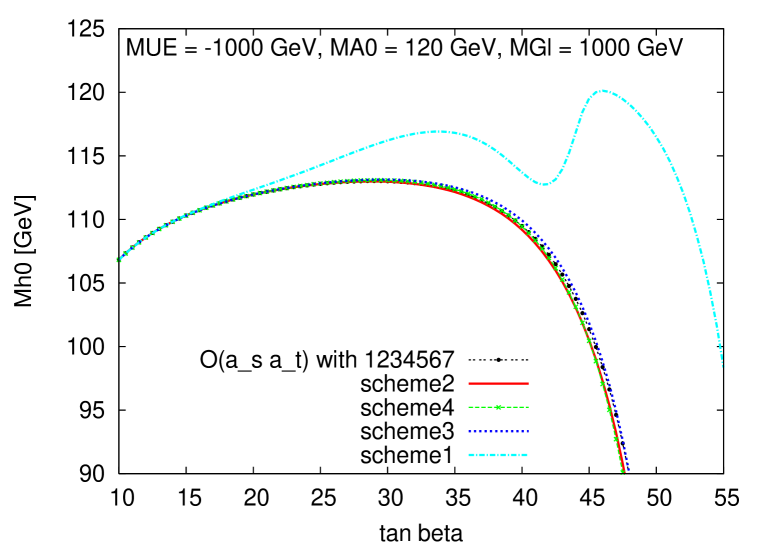
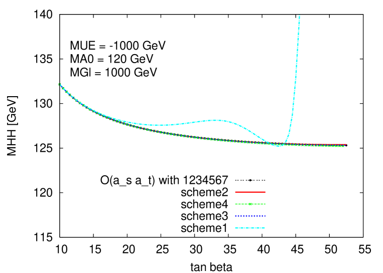
Figure 6: $\tan\beta$-dependence of $M_{h}$ and $M_{H}$ for $M_{A}=120\,\,{\rm GeV}$ and $\mu$ negative.

We start our analysis of the different renormalisation schemes by comparing the results for $M_{h}$ and $M_{H}$ as a function of $\tan\beta$ in Fig. 6. The other parameters are as given in Tab. 2. As expected from the discussion of Tab. 3 and Tab. 4, the “$m_{b}$ OS” scheme gives rise to artificially large corrections and shows very large deviations from the other schemes for intermediate and large values of $\tan\beta$. This behaviour is even more pronounced for $M_{H}$ than for $M_{h}$, as can be seen in the lower plot of Fig. 6. These extremely large corrections are a consequence of the large contributions to the counterterm of the parameter $A_{b}$ (see (59)). The Higgs self-energy contribution from virtual sbottoms contains a term proportional to $A_{b}^{2}$. Using as input a value for $A_{b}$ according to (58), very large contributions proportional to $(\delta A_{b})^{2}$ are introduced. These corrections are more pronounced in $\Sigma_{HH}$, where they enter like $(\cos\alpha\hskip 2.84526ptA_{b})^{2}$, than in $\Sigma_{hh}$, where they enter like $(\sin\alpha\hskip 2.84526ptA_{b})^{2}$ ($|\alpha|\ll 1$ in our analysis). The unacceptably large contributions to $\delta A_{b}$ in the “$m_{b}$ OS” scheme invalidate a perturbative treatment in this scheme. We therefore discard this scheme in the following and focus our discussion on the other three schemes defined in Tab. 1.

The other schemes all give similar and numerically well-behaved results, where $M_{h}$ starts to decrease rapidly with $\tan\beta$ for $\tan\beta\;\raisebox{-3.00003pt}{$\stackrel{{\scriptstyle\displaystyle>}}{{\sim}}$}\;40$. Negative mass squares are reached at $\tan\beta\simeq 53$. The main effect comes from the leading contributions of ${\cal O}(\alpha_{b}\alpha_{s})$ that enter via the resummation of $\Delta m_{b}$, see (54). The decrease with increasing $\tan\beta$ is mainly due to the dependence of $\Delta m_{b}\sim\mu\tan\beta$ in (55). The subleading ${\cal O}(\alpha_{b}\alpha_{s})$ corrections, which arise from the genuine two-loop diagrams, are of ${\cal O}(1\,\,{\rm GeV})$. The differences between the three renormalisation schemes are of similar size. For this particular parameter choice the “$A_{b}$, $\theta_{\tilde{b}}$ $\overline{\rm{DR}}$” scheme enhances $M_{h}$, whereas the other two schemes decrease $M_{h}$ compared to the case where the genuine two-loop corrections are omitted.

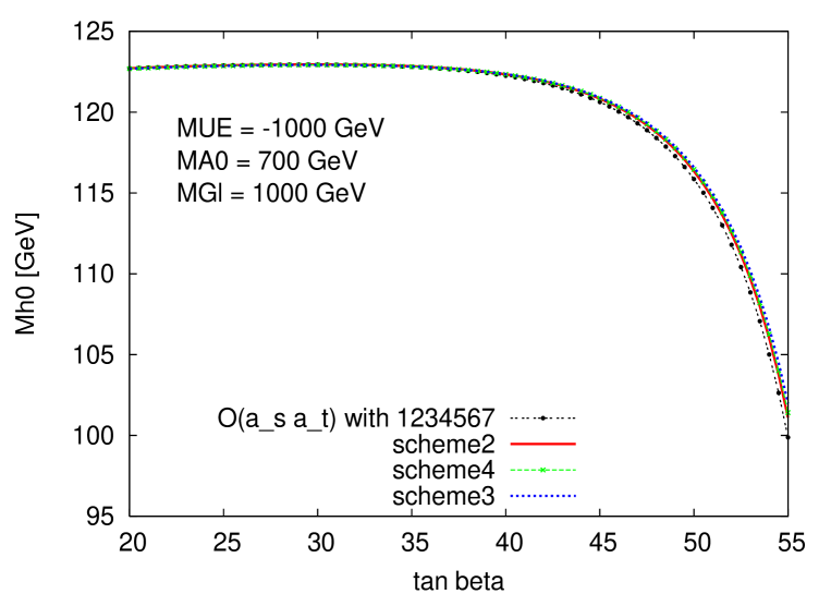
Figure 7: $\tan\beta$-dependence of $M_{h}$ for $M_{A}=700\,\,{\rm GeV}$ and $\mu$ negative.

In Fig. 7 we show $M_{h}$ as a function of $\tan\beta$ for the same parameters as in Fig. 6, but with $M_{A}=700\,\,{\rm GeV}$. This results in general in larger $M_{h}$ values, but the general behaviour as a function of $\tan\beta$ is the same as for $M_{A}=120\,\,{\rm GeV}$; $M_{h}$ drops steeply for large $\tan\beta$ values. In all three schemes the subleading terms increase $M_{h}$ by a few GeV, depending on $\tan\beta$.

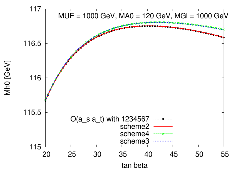
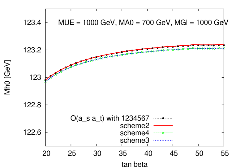
Figure 8: $\tan\beta$-dependence of $M_{h}$ for $M_{A}=120\,\,{\rm GeV}$ (upper plot) and $M_{A}=700\,\,{\rm GeV}$ (lower plot) for positive $\mu$.

As discussed above, large corrections from the $b/\tilde{b}$ sector are only expected for negative values of $\mu$. In Fig. 8 we show the results for $M_{h}$ as a function of $\tan\beta$ with positive $\mu$ and $M_{A}=120$ and $700\,\,{\rm GeV}$, respectively. The other parameters are given in Tab. 2. The positive sign of $\mu$ results in a positive $\Delta m_{b}$ and thus a smaller numerical value of $m_{b}^{\overline{\rm{DR}},\text{MSSM}}$. As expected, the variation of $M_{h}$ with $\tan\beta$ is much smaller than for negative $\mu$. Both, the leading corrections, i.e. the $\tan\beta$ enhanced terms of ${\cal O}(\alpha_{b}\alpha_{s})$, as well as the subleading corrections are at the level of ${\cal O}(100\,\,{\rm MeV})$. The “$m_{b}$ $\overline{\rm{DR}}$” scheme does not show any visible corrections beyond the resummed contributions. This leads to the conclusion that for positive $\mu$ the corrections beyond the one-loop level coming from the $b/\tilde{b}$ sector are sufficiently well under control. However, in view of the fact that the anticipated ILC accuracy on $M_{h}$ [7, 8, 9] and the parametric uncertainty of the theory prediction from the ILC measurement of the top-quark mass [54, 55] will both be about 100 MeV, ultimately the aim will be to reduce the theoretical uncertainties from unknown higher-order corrections to at least this level. This will require the inclusion of all two-loop corrections (and a significant part of corrections beyond two-loop order). For the further analysis in this paper we focus on negative values of $\mu$.

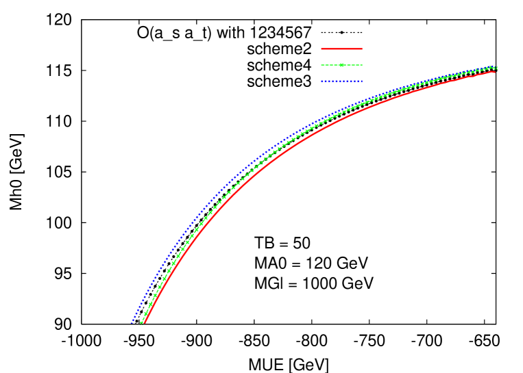
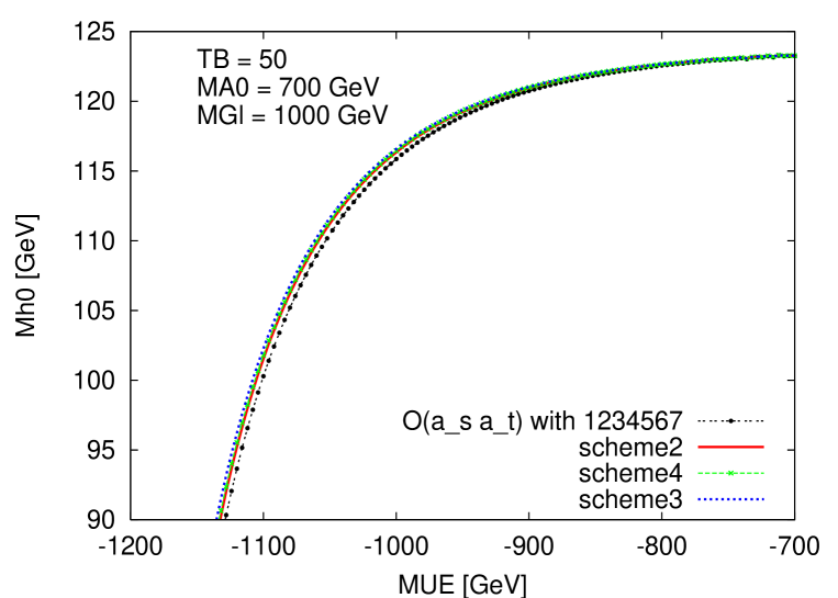
Figure 9: $\mu$-dependence of $M_{h}$ for $M_{A}=120\,\,{\rm GeV}$ (upper plot) and $M_{A}=700\,\,{\rm GeV}$ (lower plot) for $\tan\beta=50$.

The variation of $M_{h}$ with $\mu$ (for $\mu<0$) for $\tan\beta=50$ is shown in Fig. 9. As can be expected from (55) the corrections at ${\cal O}(\alpha_{b}\alpha_{s})$ increase with increasing $|\mu|$. Typically the genuine two-loop contributions are of ${\cal O}(1\,\,{\rm GeV})$. For large $M_{A}$ all the schemes lead to an increase of $M_{h}$, whereas for small $M_{A}$ both negative and positive shifts can occur. Differences in the $M_{h}$ predictions induced by the different renormalisation schemes are below the GeV level for large $M_{A}$.

In Fig. 10 the dependence of $M_{h}$ on $M_{A}$ is shown for the different renormalisation schemes, with the other default parameters from Tab. 2. For $M_{A}\;\raisebox{-3.00003pt}{$\stackrel{{\scriptstyle\displaystyle>}}{{\sim}}$}\;200\,\,{\rm GeV}$ the subleading terms of all three schemes enhance $M_{h}$ by ${\cal O}(1\,\,{\rm GeV})$. A decrease only occurs for small values of $M_{A}$, depending on the scheme. The differences in the $M_{h}$ prediction resulting from the use of different renormalisation schemes decrease for $M_{A}\;\raisebox{-3.00003pt}{$\stackrel{{\scriptstyle\displaystyle>}}{{\sim}}$}\;200\,\,{\rm GeV}$ to ${\cal O}(0.1\,\,{\rm GeV})$.

Figure 10: $M_{A}$-dependence of $M_{h}$ for $\tan\beta=50$ and $\mu$ negative.

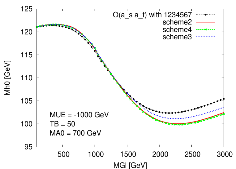
Figure 11: $m_{\tilde{g}}$-dependence of $M_{h}$ for $M_{A}=700\,\,{\rm GeV}$, $\tan\beta=50$ and $\mu$ negative.

In Fig. 11 it can be seen that the behaviour of the corrections strongly depends on the choice of $m_{\tilde{g}}$. The figure shows $M_{h}$ as a function of $m_{\tilde{g}}$ for $\mu=-1000\,\,{\rm GeV}$, $\tan\beta=50$ and $M_{A}=700\,\,{\rm GeV}$. For $m_{\tilde{g}}\;\raisebox{-3.00003pt}{$\stackrel{{\scriptstyle\displaystyle<}}{{\sim}}$}\;1000\,\,{\rm GeV}$ all schemes lead to an increase of $M_{h}$ from the subleading ${\cal O}(\alpha_{b}\alpha_{s})$ corrections. For $m_{\tilde{g}}\;\raisebox{-3.00003pt}{$\stackrel{{\scriptstyle\displaystyle>}}{{\sim}}$}\;1500\,\,{\rm GeV}$, on the other hand, all schemes lead to a decrease, where the size of the individual corrections also strongly varies with $m_{\tilde{g}}$. Accordingly, the relative size of the corrections in the different schemes also varies with $m_{\tilde{g}}$. Corrections up to about $3\,\,{\rm GeV}$ are possible. The differences between the three schemes are of ${\cal O}(2\,\,{\rm GeV})$ for large $m_{\tilde{g}}$. It should be noted that the effects of the higher-order corrections to $M_{h}$ do not decouple with large $m_{\tilde{g}}$. The corrections at ${\cal O}(\alpha_{t}\alpha_{s})$ [19] as well as ${\cal O}(\alpha_{b}\alpha_{s})$ grow logarithmically in the renormalisation schemes that we have adopted.

The above analysis of the three schemes “$m_{b}$ $\overline{\rm{DR}}$”, “$A_{b}$, $\theta_{\tilde{b}}$ $\overline{\rm{DR}}$”, and “$A_{b}$, $\theta_{\tilde{b}}$ OS” in various parameter regions yields numerically well-behaved and physically meaningful results. As there is no clear preference for one of the schemes on physical grounds, the difference between the results obtained in the three schemes can be interpreted as an indication of the possible size of missing higher-order corrections. The size of the individual corrections and also the differences between the renormalisation schemes sensitively depend on the input parameters. Typically we find that the genuine two-loop corrections in the $b/\tilde{b}$ sector yield a shift in $M_{h}$ of ${\cal O}(1\,\,{\rm GeV})$. The differences between the three schemes are usually somewhat smaller.

4.3 Numerical analysis of the renormalisation scale dependence

While in the previous section we compared the results of different renormalisation scheme, we now focus on the “$m_{b}$ $\overline{\rm{DR}}$” scheme and investigate the effect of varying the renormalisation scale of the ${\cal O}(\alpha_{b}\alpha_{s})$ result obtained in this scheme. We vary the scale within the interval $m_{t}/2\leq\mu^{\overline{\rm{DR}}}\leq 2\,m_{t}$, resulting in a shift which is formally of ${\cal O}(\alpha_{b}\alpha_{s}^{2})$. The results are shown as a function of $m_{\tilde{g}}$ for $\tan\beta=50$ in Fig. 12 for $M_{A}=120\,\,{\rm GeV}$ and $M_{A}=700\,\,{\rm GeV}$.

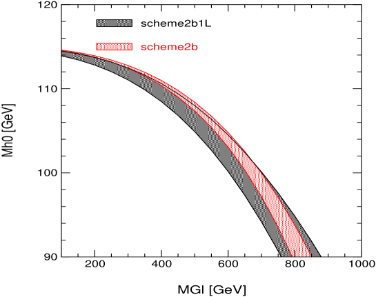
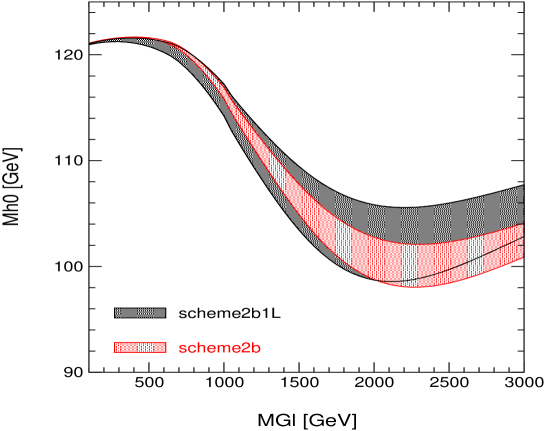
Figure 12: $\mu^{\overline{\rm{DR}}}$ dependence of $M_{h}$ as a function of $m_{\tilde{g}}$ for $M_{A}=120\,\,{\rm GeV}$ (upper plot) and $M_{A}=700\,\,{\rm GeV}$ (lower plot) for $\mu=-1000\,\,{\rm GeV}$, $\tan\beta=50$. The black area corresponds to the ${\cal O}(\alpha_{t}\alpha_{s})$ result including resummation, i.e. the result without the subleading two-loop ${\cal O}(\alpha_{b}\alpha_{s})$ terms.

The $\mu^{\overline{\rm{DR}}}$ variation of the leading contribution (the ${\cal O}(\alpha_{t}\alpha_{s})$ result including resummation) is shown as the dark shaded (black) band. The results including the subleading corrections in the “$m_{b}$ $\overline{\rm{DR}}$” scheme are shown as a light shaded (red) band. It can be seen that the variation with $\mu^{\overline{\rm{DR}}}$ is strongly reduced by the inclusion of the subleading contributions. The variation with $\mu^{\overline{\rm{DR}}}$ within the “$m_{b}$ $\overline{\rm{DR}}$” scheme is tiny for $m_{\tilde{g}}\;\raisebox{-3.00003pt}{$\stackrel{{\scriptstyle\displaystyle<}}{{\sim}}$}\;500\,\,{\rm GeV}$, and reaches $\pm 2\,\,{\rm GeV}$ for large $m_{\tilde{g}}$ values. Thus, the $\mu^{\overline{\rm{DR}}}$ variation causes a similar shift in $M_{h}$ as the comparison between the three renormalisation schemes discussed above.

We have also analysed the variation with $\mu^{\overline{\rm{DR}}}$ in the case $\mu>0$, which is not shown here. As for negative $\mu$, the variation with $\mu^{\overline{\rm{DR}}}$ is of the same order as the differences between the three renormalisation schemes, see Fig. 8. Therefore, for $\mu>0$ the unknown higher-order corrections to $M_{h}$ from the $b/\tilde{b}$ sector can be estimated to be of ${\cal O}(100\,\,{\rm MeV})$.

4.4 Comparison with existing calculations

Finally we compare our result with the existing calculation of the ${\cal O}(\alpha_{b}\alpha_{s})$ corrections presented in Ref. [26]. The renormalisation employed there consists of an on-shell renormalisation of the two scalar bottom masses and the on-shell condition for $A_{b}$ shown in Sect. 3.2.4. We denote it as “$m_{\tilde{b}},\;A_{b}$ OS” renormalisation. Thus, the differences between our “$A_{b},\;\theta_{\tilde{b}}$ OS” and the “$m_{\tilde{b}},\;A_{b}$ OS” renormalisation are the different treatment of the $m_{\tilde{b}_{1}}$ renormalisation, as well as the treatment of $\tan\beta$. We kept $\tan\beta$ as a free parameter, whereas in Ref. [26] it was set to infinity in the subleading ${\cal O}(\alpha_{b}\alpha_{s})$ corrections. In Ref. [26] the shift of the sbottom masses due to the SU(2)-invariance was taken into account in the numerical evaluation of the sbottom masses following the prescription in Ref. [56] (see also Ref. [42]).

Our result for $M_{h}$ in the “$A_{b},\;\theta_{\tilde{b}}$ OS” scheme is compared with the result of Ref. [26] in Fig. 13. For the implementation of the latter (“$m_{\tilde{b}},\;A_{b}$ OS” scheme) the Fortran code of Ref. [26] for the numerical evaluation of the $\mathcal{O}(\alpha_{s}\alpha_{b})$ corrections to the Higgs-boson self-energies has been used [57]. Thereby the input values were determined according to (57) and (58). Using these input values for $A_{b}$ and $m_{b}$ the sbottom masses were calculated taking the sbottom mass shift into account [56]. $M_{h}$ is shown as function of $m_{\tilde{g}}$ for $\mu<0$, $\tan\beta=50$, and $M_{A}=700\,\,{\rm GeV}$. Our result in the “$A_{b},\;\theta_{\tilde{b}}$ OS” scheme is shown as the dash-star (green) curve, while the result of Ref. [26] (“$m_{\tilde{b}},\;A_{b}$ OS” scheme) is given by the fine-dotted (pink) curve. The leading contribution in the two schemes, i.e. the ${\cal O}(\alpha_{t}\alpha_{s})$ result including resummation, is also shown: the light-dot-dashed (orange) curve shows the ${\cal O}(\alpha_{t}\alpha_{s})$ result using the “$A_{b},\;\theta_{\tilde{b}}$ OS” renormalised parameters; the corresponding result for the “$m_{\tilde{b}},\;A_{b}$ OS” renormalised parameters is shown as the light-dotted (gray) curve.

Fig. 13 shows that the ${\cal O}(\alpha_{t}\alpha_{s})$ results in the two schemes differ from each other by up to $2\,\,{\rm GeV}$ for large $m_{\tilde{g}}$. The inclusion of the subleading two-loop corrections reduces this difference significantly. Our result in the “$A_{b},\;\theta_{\tilde{b}}$ OS” scheme agrees with the result of Ref. [26] to better than $0.5\,\,{\rm GeV}$.

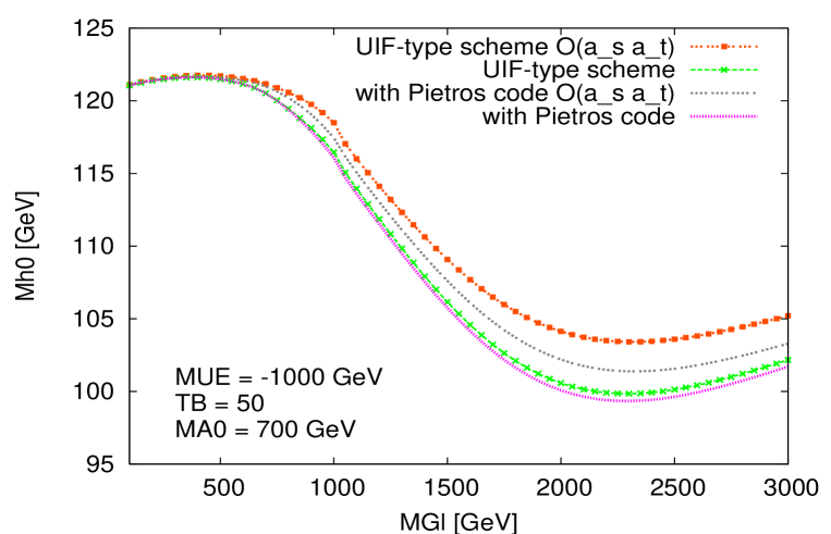
Figure 13: Comparison of our ${\cal O}(\alpha_{b}\alpha_{s})$ result for $M_{h}$ in the “$A_{b},\;\theta_{\tilde{b}}$ OS” scheme and the result of Ref. [26] (“$m_{\tilde{b}},\;A_{b}$ OS” scheme) as a function of $m_{\tilde{g}}$. The ${\cal O}(\alpha_{t}\alpha_{s})$ results in the two schemes, where the subleading ${\cal O}(\alpha_{b}\alpha_{s})$ corrections are omitted (using the appropriate renormalised parameters), are also shown.

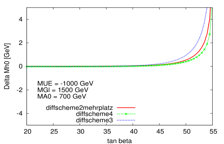
Figure 14: Comparison of our ${\cal O}(\alpha_{b}\alpha_{s})$ result in three different renormalisation schemes and the result of Ref. [26]. The three curves for $\Delta M_{h}$ show the difference between our result in each of the three schemes and the result of Ref. [26] as a function of $\tan\beta$.

In Fig. 14 we compare our result in each of the three schemes discussed above, i.e. the “$A_{b},\;\theta_{\tilde{b}}$ OS”, the “$m_{b}$ $\overline{\rm{DR}}$” and the “$A_{b}$, $\theta_{\tilde{b}}$ $\overline{\rm{DR}}$” schemes, with the result of Ref. [26]. The difference $\Delta M_{h}$ between our result and the result of Ref. [26] is shown for each of the three schemes as a function of $\tan\beta$ for $m_{\tilde{g}}=1500\,\,{\rm GeV}$, $\mu=-1000\,\,{\rm GeV}$, and $M_{A}=700\,\,{\rm GeV}$. The differences stay below $1\,\,{\rm GeV}$ for $\tan\beta\;\raisebox{-3.00003pt}{$\stackrel{{\scriptstyle\displaystyle<}}{{\sim}}$}\;50$, where our result in the “$A_{b}$, $\theta_{\tilde{b}}$ $\overline{\rm{DR}}$” scheme shows the biggest deviation from the result of Ref. [26], while as expected, the difference is smallest for the “$A_{b}$, $\theta_{\tilde{b}}$ OS” scheme. For $\tan\beta>50$ large deviations occur because of the sharp decrease of $M_{h}$ in this region (see e.g. Fig. 7).

5 Conclusions

We have obtained results for the two-loop ${\cal O}(\alpha_{b}\alpha_{s})$ corrections to the neutral ${\cal CP}$-even Higgs-boson masses in the MSSM within different renormalisation schemes. The leading $\tan\beta$-enhanced contributions of the $b/\tilde{b}$ sector can be incorporated into an appropriately chosen bottom Yukawa coupling, for which we use the bottom-quark mass in the $\overline{\rm{DR}}$ scheme with a resummation of the leading contributions. We have analysed in detail the impact of the genuine (subleading) ${\cal O}(\alpha_{b}\alpha_{s})$ two-loop corrections in different parts of the MSSM parameter space and we have compared the results obtained in the different schemes.

We have shown that an on-shell scheme that is frequently used in the $t/\tilde{t}$ sector leads to numerically unstable results if it is applied in the $b/\tilde{b}$ sector. The origin of the huge corrections in this scheme was traced to the fact that it involves a renormalisation condition for the sbottom mixing angle, $\theta_{\tilde{b}}$, rather than for the trilinear coupling, $A_{b}$.

The other three schemes that we have analysed yield numerically well-behaved and physically meaningful results. For $\mu>0$ the effect of the genuine ${\cal O}(\alpha_{b}\alpha_{s})$ two-loop corrections is rather small, typically of ${\cal O}(100\,\,{\rm MeV})$. Corrections at this level will nevertheless be relevant in view of the prospective accuracy of measurements in the Higgs sector and of the top-quark mass at the ILC. For $\mu<0$ the effective bottom Yukawa coupling increases, leading to an enhancement of the effects from the $b/\tilde{b}$ sector. While the constraints arising from the measurement of the anomalous magnetic moment of the muon favour the positive sign of $\mu$, it seems premature at the present stage to discard the parameter region with $\mu<0$. For large values of $\tan\beta$ and $m_{\tilde{g}}$ and large negative values of $\mu$ we find that the genuine ${\cal O}(\alpha_{b}\alpha_{s})$ corrections can amount up to $3\,\,{\rm GeV}$. We have compared our result for the ${\cal O}(\alpha_{b}\alpha_{s})$ corrections with the existing result in the literature, which was obtained in the limit of $\tan\beta\to\infty$, and found good agreement.

The comparison of the results in the different schemes that we have analysed and the investigation of the renormalisation scale dependence give an indication of the possible size of missing higher-order corrections in the $b/\tilde{b}$ sector. For $\mu>0$ the higher-order corrections from the $b/\tilde{b}$ sector (beyond ${\cal O}(\alpha_{b}\alpha_{s})$) appear to be sufficiently well under control even in view of the prospective ILC accuracy. This applies especially to the “$m_{b}$ $\overline{\rm{DR}}$” scheme, where the corrections beyond the improved one-loop result have been found to be particularly small. For $\mu<0$, on the other hand, sizable higher-order corrections from the $b/\tilde{b}$ sector are possible. The size of the individual corrections and also the difference between the analysed schemes varies significantly with the relevant parameters, $\mu$, $\tan\beta$, $m_{\tilde{g}}$ and $M_{A}$. We estimate the uncertainty from missing higher-order corrections in the $b/\tilde{b}$ sector to be about $2\,\,{\rm GeV}$ in this region of parameter space.

The results obtained will be implemented into the Fortran code FeynHiggs [58, 59]. The evaluation of the results within the three schemes will allow to obtain an estimate of the size of the missing higher-order corrections as a function of the chosen input parameters.

Acknowledgements

We thank A. Hoang, U. Nierste, P. Slavich and D. Stöckinger for helpful discussions. We are grateful to P. Slavich for providing the Fortran code for the “$m_{\tilde{b}}$, $A_{b}$ OS” renormalisation scheme. S.H. and G.W. thank the Max Planck Institut für Physik, München, for kind hospitality during part of this work. G.W. thanks the CERN theory group for kind hospitality during the final stage of this paper. This work has been supported by the European Community’s Human Potential Programme under contract HPRN-CT-2000-00149 “Physics at Colliders”.

Appendix: Counterterms of the quark/squark sector

In section 3 the counterterms have been given using the definitions (20) and (22) for the sfermion masses and mixing angles. In this appendix the counterterms are given in a more general way allowing to use also other definitions for the sfermion masses and mixing angles. Introducing a counterterm for the mixing angle needs a certain choice of definitions of the sfermion masses and mixing angles. Instead of using an explicit mixing angle counterterm the counterterm $\delta Y_{\tilde{q}}$ is introduced as

$$\delta Y_{\tilde{q}}=({\cal U}_{\tilde{q}}\delta{\cal M}_{\tilde{q}}{\cal U}^{\dagger}_{\tilde{q}})_{12}=({\cal U}_{\tilde{q}}\delta{\cal M}_{\tilde{q}}{\cal U}^{\dagger}_{\tilde{q}})_{21}~{},$$ (60)

where the counterterm mass matrix $\delta{\cal M}_{\tilde{q}}$ contains the counterterms of the parameters appearing in (19). With the definitions (20) and (22) $\delta Y_{\tilde{q}}$ is related to the mixing angle counterterm as follows

$$\delta Y_{\tilde{q}} =(m_{\tilde{q}_{1}}^{2}-m_{\tilde{q}_{2}}^{2})\,\delta\theta\kern-1.49994pt_{\tilde{q}}\,.$$ (61)

$\bullet$ Top quark/squark sector:

The counterterms for the top-quark mass (24) and the stop masses (26) are already in a general form. The counterterm for the mixing angle (27) is replaced by

$$\delta Y_{\tilde{t}}=\frac{1}{2}\Bigl{(}\mathop{\rm Re}\Sigma_{\tilde{t}_{12}}(m_{{\tilde{t}}_{1}}^{2})+\mathop{\rm Re}\Sigma_{\tilde{t}_{12}}(m_{{\tilde{t}}_{2}}^{2})\Bigr{)},$$ (62)

and the counterterm of the A-parameter (29) is rewritten as

$$\delta A_{t} =\frac{1}{m_{t}}\Bigl{[}U_{\tilde{t}_{11}}U_{\tilde{t}_{12}}\bigl{(}\delta m_{\tilde{t}_{1}}^{2}-\delta m_{\tilde{t}_{2}}^{2}\bigr{)}+(U_{\tilde{t}_{11}}U_{\tilde{t}_{22}}+U_{\tilde{t}_{12}}U_{\tilde{t}_{21}})\,\delta Y_{\tilde{t}}-\delta m_{t}\,(A_{t}-\mu\cot\beta)\Bigr{]}~{}.$$ (63)

$\bullet$ Analogous to the top quark/squark sector:

As in the top quark/squark sector the counterterm for the mixing angle (36) is replaced by

$$\delta Y_{\tilde{b}}=\frac{1}{2}\Bigl{(}\mathop{\rm Re}\Sigma_{\tilde{b}_{12}}(m_{\tilde{b}_{1}}^{2})+\mathop{\rm Re}\Sigma_{\tilde{b}_{12}}(m_{\tilde{b}_{2}}^{2})\Bigr{)}\;.$$ (64)

The dependent counterterms of the $\tilde{b}_{1}$-mass (32) and of the A-parameter (37) are rewritten as follows:

$$\delta m_{\tilde{b}_{1}}^{2} =\frac{1}{U_{\tilde{b}_{11}}^{2}}\bigl{[}-U_{\tilde{b}_{12}}^{2}\delta m_{\tilde{b}_{2}}^{2}+2U_{\tilde{b}_{12}}U_{\tilde{b}_{22}}\delta Y_{\tilde{b}}+U_{\tilde{t}_{11}}^{2}\delta m_{\tilde{t}_{1}}^{2}+U_{\tilde{t}_{12}}^{2}\delta m_{\tilde{t}_{2}}^{2}$$

$$\quad\ -2U_{\tilde{t}_{12}}U_{\tilde{t}_{22}}\delta Y_{\tilde{t}}+(2m_{b}\delta m_{b}-2m_{t}\delta m_{t})\bigr{]}~{},$$ (65)

$$\delta A_{b} =\frac{1}{m_{b}}\Bigl{[}-\frac{U_{\tilde{b}_{12}}}{U_{\tilde{b}_{11}}}\delta m_{\tilde{b}_{2}}^{2}+\frac{U_{\tilde{b}_{22}}}{U_{\tilde{b}_{11}}}\delta Y_{\tilde{b}}-\delta m_{b}(A_{b}-\mu\tan\beta-2\frac{U_{\tilde{b}_{12}}}{U_{\tilde{b}_{11}}}m_{b})$$

$$\quad\ \quad\ +\frac{U_{\tilde{b}_{12}}}{U_{\tilde{b}_{11}}}\bigl{(}U_{\tilde{t}_{11}}^{2}\delta m_{\tilde{t}_{1}}^{2}+U_{\tilde{t}_{12}}^{2}\delta m_{\tilde{t}_{2}}^{2}-2U_{\tilde{t}_{12}}U_{\tilde{t}_{22}}\delta Y_{\tilde{t}}-2m_{t}\delta m_{t}\bigr{)}\Bigr{]}~{}.$$ (66)

$\bullet$ $\overline{\rm{DR}}$ bottom-quark mass

The A-parameter counterterm (40) is written in the following way

$$\delta A_{b} =\frac{1}{m_{b}}\Bigl{[}-\frac{U_{\tilde{b}_{12}}}{U_{\tilde{b}_{11}}}\mathop{\rm Re}\Sigma_{\tilde{b}_{22}}^{\rm div}(m_{\tilde{b}_{2}}^{2})+\frac{U_{\tilde{b}_{22}}}{2U_{\tilde{b}_{11}}}\bigl{(}\mathop{\rm Re}\Sigma_{\tilde{b}_{12}}^{\rm div}(m_{\tilde{b}_{1}}^{2})+\mathop{\rm Re}\Sigma_{\tilde{b}_{12}}^{\rm div}(m_{\tilde{b}_{2}}^{2})\bigr{)}$$

$$\quad\quad\ +\frac{U_{\tilde{b}_{12}}}{U_{\tilde{b}_{11}}}\Bigl{(}U_{\tilde{t}_{11}}^{2}\mathop{\rm Re}\Sigma_{\tilde{t}_{11}}^{\rm div}(m_{\tilde{t}_{1}}^{2})+U_{\tilde{t}_{12}}^{2}\mathop{\rm Re}\Sigma_{\tilde{t}_{22}}^{\rm div}(m_{\tilde{t}_{2}}^{2})$$

$$\quad\quad\ -U_{\tilde{t}_{12}}U_{\tilde{t}_{22}}\bigl{(}\mathop{\rm Re}\Sigma_{\tilde{t}_{12}}^{\rm div}(m_{\tilde{t}_{1}}^{2})+\mathop{\rm Re}\Sigma_{\tilde{t}_{12}}^{\rm div}(m_{\tilde{t}_{2}}^{2})\bigr{)}$$

$$\quad\quad\ -m_{t}^{2}(\mathop{\rm Re}{\Sigma}_{{t}_{L}}^{\rm div}(m_{t}^{2})+\mathop{\rm Re}{\Sigma}_{{t}_{R}}^{\rm div}(m_{t}^{2})+2\mathop{\rm Re}{\Sigma}_{{t}_{S}}^{\rm div}(m_{t}^{2}))\Bigr{)}\Bigr{]}+\frac{1}{2}(2\frac{U_{\tilde{b}_{12}}}{U_{\tilde{b}_{11}}}m_{b}$$

$$\quad\quad-A_{b}+\mu\tan\beta)\Bigl{(}\mathop{\rm Re}{\Sigma}_{{b}_{L}}^{\rm div}(m_{b}^{2})+\mathop{\rm Re}{\Sigma}_{{b}_{R}}^{\rm div}(m_{b}^{2})+2\mathop{\rm Re}{\Sigma}_{{b}_{S}}^{\rm div}(m_{b}^{2})\Bigr{)}~{},$$ (67)

avoiding an explicit definition of the mixing angles. The dependent counterterm for the mixing angle (41) is replaced by

$$\delta Y_{\tilde{b}} =\frac{U_{\tilde{b}_{11}}}{U_{\tilde{b}_{22}}}m_{b}\delta A_{b}+\frac{U_{\tilde{b}_{11}}}{U_{\tilde{b}_{22}}}\delta m_{b}(A_{b}-\mu\tan\beta-2\frac{U_{\tilde{b}_{12}}}{U_{\tilde{b}_{11}}}m_{b})+\frac{U_{\tilde{b}_{12}}}{U_{\tilde{b}_{22}}}\bigl{[}\delta m_{\tilde{b}_{2}}^{2}$$

$$\quad\ -U_{\tilde{t}_{11}}^{2}\delta m_{\tilde{t}_{1}}^{2}-U_{\tilde{t}_{12}}^{2}\delta m_{\tilde{t}_{2}}^{2}+2U_{\tilde{t}_{12}}U_{\tilde{t}_{22}}\delta Y_{\tilde{t}}+2m_{t}\delta m_{t}\bigr{]}~{},$$ (68)

and the counterterm for the $\tilde{b}_{1}$-mass (42) by

$$\delta m_{\tilde{b}_{1}}^{2} =\frac{1}{U_{\tilde{b}_{11}}^{2}}\Bigl{[}(1-2U_{\tilde{b}_{12}}^{2})\Bigl{(}U_{\tilde{t}_{11}}^{2}\delta m_{\tilde{t}_{1}}^{2}+U_{\tilde{t}_{12}}^{2}\delta m_{\tilde{t}_{2}}^{2}-2U_{\tilde{t}_{12}}U_{\tilde{t}_{22}}\delta Y_{\tilde{t}}-2m_{t}\delta m_{t}\Bigr{)}+U_{\tilde{b}_{12}}^{2}\delta m_{\tilde{b}_{2}}^{2}$$

$$\quad+2U_{\tilde{b}_{11}}U_{\tilde{b}_{12}}m_{b}\delta A_{b}+\Bigl{(}2U_{\tilde{b}_{12}}U_{\tilde{b}_{11}}(A_{b}-\mu\tan\beta)+2(1-2U_{\tilde{b}_{12}}^{2})m_{b}\Bigr{)}\delta m_{b}\Bigr{]}~{}.$$ (69)

$\bullet$ $\overline{\rm{DR}}$ mixing angle and $A_{b}$

The counterterm for the mixing angle (46) is replaced by

$$\delta Y_{\tilde{b}}=\frac{1}{2}\bigl{(}\mathop{\rm Re}\Sigma_{\tilde{b}_{12}}^{\rm div}(m_{\tilde{b}_{1}}^{2})+\mathop{\rm Re}\Sigma_{\tilde{b}_{12}}^{\rm div}(m_{\tilde{b}_{2}}^{2})\bigr{)}\;.$$ (70)

The dependent counterterm for the bottom quark mass (47) is rewritten as the following combination of counterterms:

$$\delta m_{b} =-\Bigl{[}m_{b}\,\delta A_{b}-\frac{U_{\tilde{b}_{22}}}{U_{\tilde{b}_{11}}}\delta Y_{\tilde{b}}+\frac{U_{\tilde{b}_{12}}}{U_{\tilde{b}_{11}}}\delta m_{\tilde{b}_{2}}^{2}-\frac{U_{\tilde{b}_{12}}}{U_{\tilde{b}_{11}}}\Bigl{(}U_{\tilde{t}_{11}}^{2}\delta m_{\tilde{t}_{1}}^{2}+U_{\tilde{t}_{12}}^{2}\delta m_{\tilde{t}_{2}}^{2}-2U_{\tilde{t}_{12}}U_{\tilde{t}_{22}}\delta Y_{\tilde{t}}$$

$$\quad\ -2m_{t}\,\delta m_{t}\Bigr{)}\Bigr{]}\Bigl{[}A_{b}-\mu\tan\beta-2m_{b}\frac{U_{\tilde{b}_{12}}}{U_{\tilde{b}_{11}}}\Bigr{]}^{-1}~{}.$$ (71)

The counterterm for the $\tilde{b}_{1}$-mass is obtained by inserting the expression (71) for the bottom quark mass into the expression (65).

$\bullet$ On-shell mixing angle and $A_{b}$

The renormalised vertex (50) has the following general form

$$\hat{\Lambda}(p_{A}^{2},p_{\tilde{b}_{1}}^{2},p_{\tilde{b}_{2}}^{2}) =\Lambda(p_{A}^{2},p_{\tilde{b}_{1}}^{2},p_{\tilde{b}_{2}}^{2})+\frac{ie}{2M_{W}\sin\theta_{W}}(U_{\tilde{b}_{11}}U_{\tilde{b}_{22}}-U_{\tilde{b}_{12}}U_{\tilde{b}_{21}})\Bigl{[}m_{b}\tan\beta\delta A_{b}$$

$$\quad+(\mu+\tan\beta A_{b})\Bigl{(}\delta m_{b}+\frac{1}{2}m_{b}(\delta Z_{\tilde{b}_{1}\tilde{b}_{1}}+\delta Z_{\tilde{b}_{2}\tilde{b}_{2}})\Bigr{)}\Bigr{]}~{}.$$ (72)

Using the renormalisation condition (49) the counterterms of the A-parameter and the bottom quark mass can be derived as

$$\delta A_{b} =i\frac{M_{W}\sin\theta_{W}}{e\,m_{b}\tan\beta(U_{\tilde{b}_{11}}U_{\tilde{b}_{22}}-U_{\tilde{b}_{12}}U_{\tilde{b}_{21}})}\Bigl{(}\Lambda(0,m_{\tilde{b}_{1}}^{2},m_{\tilde{b}_{1}}^{2})+\Lambda(0,m_{\tilde{b}_{2}}^{2},m_{\tilde{b}_{2}}^{2})\Bigr{)}$$

$$\quad-\frac{\mu+A_{b}\tan\beta}{2\tan\beta}(\delta Z_{\tilde{b}_{1}\tilde{b}_{1}}+\delta Z_{\tilde{b}_{2}\tilde{b}_{2}})$$

$$\quad-\frac{\mu+A_{b}\tan\beta}{m_{b}\tan\beta}\Bigg{[}i\frac{M_{W}\sin\theta_{W}}{e\tan\beta(U_{\tilde{b}_{11}}U_{\tilde{b}_{22}}-U_{\tilde{b}_{12}}U_{\tilde{b}_{21}})}\Bigl{(}\Lambda(0,m_{\tilde{b}_{1}}^{2},m_{\tilde{b}_{1}}^{2})+\Lambda(0,m_{\tilde{b}_{2}}^{2},m_{\tilde{b}_{2}}^{2})\Bigr{)}$$

$$\qquad-\frac{m_{b}(\mu+A_{b}\tan\beta)}{2\tan\beta}(\delta Z_{\tilde{b}_{1}\tilde{b}_{1}}+\delta Z_{\tilde{b}_{2}\tilde{b}_{2}})+\frac{U_{\tilde{b}_{12}}}{U_{\tilde{b}_{11}}}\delta m_{\tilde{b}_{2}}^{2}-\frac{U_{\tilde{b}_{22}}}{U_{\tilde{b}_{11}}}\delta Y_{\tilde{b}}-\frac{U_{\tilde{b}_{12}}}{U_{\tilde{b}_{11}}}\Bigl{(}U_{\tilde{t}_{11}}^{2}\delta m_{\tilde{t}_{1}}^{2}$$

$$\qquad+U_{\tilde{t}_{12}}^{2}\delta m_{\tilde{t}_{2}}^{2}-2U_{\tilde{t}_{12}}U_{\tilde{t}_{22}}\delta Y_{\tilde{t}}-2m_{t}\delta m_{t}\Bigr{)}\Bigg{]}\left[\mu\Bigl{(}\tan\beta+\frac{1}{\tan\beta}\Bigr{)}+2m_{b}\frac{U_{\tilde{b}_{12}}}{U_{\tilde{b}_{11}}}\right]^{-1}~{},$$ (73)

and

$$\delta m_{b} =\Bigl{[}i\frac{M_{W}\sin\theta_{W}}{e\,\tan\beta(U_{\tilde{b}_{11}}U_{\tilde{b}_{22}}-U_{\tilde{b}_{12}}U_{\tilde{b}_{21}})}\Bigl{(}\Lambda(0,m_{\tilde{b}_{1}}^{2},m_{\tilde{b}_{1}}^{2})+\Lambda(0,m_{\tilde{b}_{2}}^{2},m_{\tilde{b}_{2}}^{2})\Bigr{)}$$

$$\quad\ -\frac{m_{b}(\mu+A_{b}\tan\beta)}{2\tan\beta}(\delta Z_{\tilde{b}_{1}\tilde{b}_{1}}+\delta Z_{\tilde{b}_{2}\tilde{b}_{2}})-\frac{U_{\tilde{b}_{22}}}{U_{\tilde{b}_{11}}}\delta Y_{\tilde{b}}+\frac{U_{\tilde{b}_{12}}}{U_{\tilde{b}_{11}}}\delta m_{\tilde{b}_{2}}^{2}-\frac{U_{\tilde{b}_{12}}}{U_{\tilde{b}_{11}}}\Bigl{(}U_{\tilde{t}_{11}}^{2}\delta m_{\tilde{t}_{1}}^{2}$$

$$\qquad\ +U_{\tilde{t}_{12}}^{2}\delta m_{\tilde{t}_{2}}^{2}-2U_{\tilde{t}_{12}}U_{\tilde{t}_{22}}\delta Y_{\tilde{t}}-2m_{t}\delta m_{t}\Bigr{)}\Bigr{]}\Bigl{[}\mu\Bigl{(}\tan\beta+\frac{1}{\tan\beta}\Bigr{)}+2m_{b}\frac{U_{\tilde{b}_{12}}}{U_{\tilde{b}_{11}}}\Bigr{]}^{-1}~{},$$ (74)

replacing (51) and (53). The counterterm of the mixing angle (48) is replaced by (64).

References

-
[1]
H.P. Nilles,
Phys. Rep. 110 (1984) 1;
H.E. Haber and G.L. Kane, Phys. Rep. 117 (1985) 75;
R. Barbieri, Riv. Nuovo Cim. 11 (1988) 1. - [2] [LEP Higgs working group], Phys. Lett. B 565 (2003) 61, hep-ex/0306033.
- [3] [LEP Higgs working group], hep-ex/0107030; hep-ex/0107031; LHWG-Note 2004-01, see: lephiggs.web.cern.ch/LEPHIGGS/papers/ .
-
[4]
ATLAS Collaboration,
Detector and Physics Performance Technical Design Report,
CERN/LHCC/99-15 (1999), see:
atlasinfo.cern.ch/Atlas/GROUPS/PHYSICS/TDR/access.html ;
CMS Collaboration, see: cmsinfo.cern.ch/Welcome.html/CMSdocuments/CMSplots/ . -
[5]
D. Zeppenfeld, R. Kinnunen, A. Nikitenko and
E. Richter-Was,
Phys. Rev. D 62 (2000) 013009,
hep-ph/0002036;
A. Belyaev and L. Reina, JHEP 0208 (2002) 041, hep-ph/0205270;
M. Dührssen, ATL-PHYS-2003-030, available from cdsweb.cern.ch . - [6] M. Dührssen, S. Heinemeyer, H. Logan, D. Rainwater, G. Weiglein and D. Zeppenfeld, hep-ph/0406323.
- [7] J. Aguilar-Saavedra et al., TESLA TDR Part 3: “Physics at an Linear Collider”, hep-ph/0106315, see: tesla.desy.de/tdr/ .
- [8] T. Abe et al. [American Linear Collider Working Group Collaboration], Resource book for Snowmass 2001, hep-ex/0106056.
- [9] K. Abe et al. [ACFA Linear Collider Working Group Collaboration], hep-ph/0109166.
-
[10]
J. Ellis, G. Ridolfi and F. Zwirner,
Phys. Lett. B 257 (1991) 83;
Y. Okada, M. Yamaguchi and T. Yanagida, Prog. Theor. Phys. 85 (1991) 1;
H. Haber and R. Hempfling, Phys. Rev. Lett. 66 (1991) 1815. - [11] A. Brignole, Phys. Lett. B 281 (1992) 284.
- [12] P. Chankowski, S. Pokorski and J. Rosiek, Phys. Lett. B 286 (1992) 307; Nucl. Phys. B 423 (1994) 423, hep-ph/9303309.
- [13] A. Dabelstein, Nucl. Phys. B 456 (1995) 25, hep-ph/9503443; Z. Phys. C 67 (1995) 495, hep-ph/9409375.
- [14] R. Hempfling and A. Hoang, Phys. Lett. B 331 (1994) 99, hep-ph/9401219.
- [15] A. Hoang, Applications of Two-Loop Calculations in the Standard Model and its Minimal Supersymmetric Extension, PhD thesis, Universität Karlsruhe, Shaker Verlag, Aachen 1995.
-
[16]
M. Carena, J. Espinosa, M. Quirós and C. Wagner,
Phys. Lett. B 355 (1995) 209,
hep-ph/9504316;
M. Carena, M. Quirós and C. Wagner, Nucl. Phys. B 461 (1996) 407, hep-ph/9508343. - [17] H. Haber, R. Hempfling and A. Hoang, Z. Phys. C 75 (1997) 539, hep-ph/9609331.
- [18] S. Heinemeyer, W. Hollik and G. Weiglein, Phys. Rev. D 58 (1998) 091701, hep-ph/9803277; Phys. Lett. B 440 (1998) 296, hep-ph/9807423.
- [19] S. Heinemeyer, W. Hollik and G. Weiglein, Eur. Phys. Jour. C 9 (1999) 343, hep-ph/9812472.
-
[20]
R. Zhang, Phys. Lett. B 447 (1999) 89,
hep-ph/9808299;
J. Espinosa and R. Zhang, JHEP 0003 (2000) 026, hep-ph/9912236. - [21] G. Degrassi, P. Slavich and F. Zwirner, Nucl. Phys. B 611 (2001) 403, hep-ph/0105096.
- [22] M. Carena, H. Haber, S. Heinemeyer, W. Hollik, C. Wagner and G. Weiglein, Nucl. Phys. B 580 (2000) 29, hep-ph/0001002.
-
[23]
S. Heinemeyer, W. Hollik and G. Weiglein,
hep-ph/9910283;
J. Espinosa and R. Zhang, JHEP 0003 (2000) 026, hep-ph/9912236. - [24] J. Espinosa and R. Zhang, Nucl. Phys. B 586 (2000) 3, hep-ph/0003246.
- [25] A. Brignole, G. Degrassi, P. Slavich and F. Zwirner, Nucl. Phys. B 631 (2002) 195, hep-ph/0112177.
- [26] A. Brignole, G. Degrassi, P. Slavich and F. Zwirner, Nucl. Phys. B 643 (2002) 79, hep-ph/0206101.
- [27] G. Degrassi, A. Dedes and P. Slavich, Nucl. Phys. B 672 (2003) 144, hep-ph/0305127.
- [28] S. Martin, Phys. Rev. D 65 (2002) 116003, hep-ph/0111209; Phys. Rev. D 66 (2002) 096001, hep-ph/0206136; Phys. Rev. D 67 (2003) 095012, hep-ph/0211366; Phys. Rev. D 68 075002 (2003), hep-ph/0307101; Phys. Rev. D 70 (2004) 016005, hep-ph/0312092.
- [29] S. Martin, hep-ph/0405022.
-
[30]
T. Banks,
Nucl. Phys. B 303 (1988) 172;
L. Hall, R. Rattazzi and U. Sarid, Phys. Rev. D 50 (1994) 7048, hep-ph/9306309;
R. Hempfling, Phys. Rev. D 49 (1994) 6168;
M. Carena, M. Olechowski, S. Pokorski and C. Wagner, Nucl. Phys. B 426 (1994) 269, hep-ph/9402253. -
[31]
M. Carena, D. Garcia, U. Nierste and C. Wagner,
Nucl. Phys. B 577 (2000) 577,
hep-ph/9912516;
H. Eberl, K. Hidaka, S. Kraml, W. Majerotto and Y. Yamada, Phys. Rev. D 62 (2000) 055006, hep-ph/9912463. - [32] G. Degrassi, S. Heinemeyer, W. Hollik, P. Slavich and G. Weiglein, Eur. Phys. Jour. C 28 (2003) 133, hep-ph/0212020.
- [33] S. Heinemeyer, hep-ph/0407244.
- [34] B. Allanach, A. Djouadi, J. Kneur, W. Porod and P. Slavich, JHEP 0409 (2004) 044, hep-ph/0406166.
- [35] J. Gunion, H. Haber, G. Kane and S. Dawson, The Higgs Hunter’s Guide, Addison-Wesley, 1990.
-
[36]
J. Küblbeck, M. Böhm and A. Denner,
Comp. Phys. Comm. 60 (1990) 165;
T. Hahn, Comput. Phys. Comm. 140 (2001) 418, hep-ph/0012260;
The program is available via www.feynarts.de . - [37] T. Hahn and C. Schappacher, Comput. Phys. Comm. 143 (2002) 54, hep-ph/0105349.
-
[38]
G. Weiglein, R. Scharf and M. Böhm,
Nucl. Phys. B 416 (1994) 606,
hep-ph/9310358;
G. Weiglein, R. Mertig, R. Scharf and M. Böhm, in New Computing Techniques in Physics Research 2, ed. D. Perret-Gallix (World Scientific, Singapore, 1992), p. 617. - [39] G. ’t Hooft and M. Veltman, Nucl. Phys. B 153 (1979) 365.
-
[40]
A. Davydychev und J. Tausk,
Nucl. Phys. B 397 (1993) 123;
F. Berends und J. Tausk, Nucl. Phys. B 421 (1994) 456. - [41] W. Hollik and H. Rzehak, Eur. Phys. Jour. C 32 (2003) 127, hep-ph/0305328.
- [42] A. Djouadi, P. Gambino, S. Heinemeyer, W. Hollik, C. Jünger and G. Weiglein, Phys. Rev. Lett. 78 (1997) 3626, hep-ph/9612363; Phys. Rev. D 57 (1998) 4179, hep-ph/9710438.
- [43] S. Eidelman et al., Phys. Lett. B 592 (2004) 1.
-
[44]
W. Siegel,
Phys. Lett. B 84 (1979) 193;
D. Capper, D. Jones and P. van Nieuwenhuizen, Nucl. Phys. B 167 (1980) 479. - [45] A. El-Khadra and M. Luke, Ann. Rev. Nucl. Part. Sci. 52 (2002) 201, hep-ph/0208114.
- [46] J. Guasch, P. Häfliger and M. Spira, Phys. Rev. D 68 (2003) 115001, hep-ph/0305101.
- [47] T. Moroi, Phys. Rev. D 53 (1996) 6565 [Erratum-ibid. D 56 (1997) 4424], hep-ph/9512396.
- [48] A. Czarnecki and W. Marciano, Phys. Rev. D 64 (2001) 013014, hep-ph/0102122.
- [49] [The Muon g-2 Collaboration], Phys. Rev. Lett. 92 (2004) 161802, hep-ex/0401008.
- [50] M. Frank, Radiative corrections to the Higgs sector of the Minimal Supersymmetric Standard Model with violation, PhD thesis, Universität Karlsruhe, Rhombos Verlag, Berlin, 2003.
- [51] M. Frank, S. Heinemeyer, W. Hollik and G. Weiglein, hep-ph/0202166.
- [52] A. Freitas and D. Stöckinger, Phys. Rev. D 66 (2002) 095014, hep-ph/0205281.
- [53] P. Azzi et al. [CDF Collaborattion, D0 Collaboration], hep-ex/0404010.
- [54] S. Heinemeyer, W. Hollik and G. Weiglein, JHEP 0006 (2000) 009, hep-ph/9909540.
- [55] S. Heinemeyer, S. Kraml, W. Porod and G. Weiglein, JHEP 0309 (2003) 075, hep-ph/0306181.
- [56] A. Bartl, H. Eberl, K. Hidaka, T. Kon, W. Majerotto and Y. Yamada, Phys. Lett. B 402 (1997) 303, hep-ph/9701398.
- [57] P. Slavich, private communication.
-
[58]
S. Heinemeyer, W. Hollik and G. Weiglein,
Comp. Phys. Comm. 124 (2000) 76,
hep-ph/9812320;
hep-ph/0002213.
The codes are accessible via www.feynhiggs.de . -
[59]
M. Frank, S. Heinemeyer, W. Hollik and G. Weiglein,
hep-ph/0212037;
T. Hahn, S. Heinemeyer, W. Hollik and G. Weiglein, MPP–2003–147, appeared in the proceedings of the Physics at TeV Colliders, Les Houches, June 2003, hep-ph/0406152; in preparation.