Final–state radiation in electron–positron annihilation into a pion pair

Abstract

The process of $e^{+}e^{-}$ annihilation into a $\pi^{+}\pi^{-}$ pair with radiation of a photon is considered. The amplitude of the reaction $e^{+}e^{-}\to\pi^{+}\pi^{-}\gamma$ consists of the model independent initial-state radiation (ISR) and model dependent final-state radiation (FSR). The general structure of the FSR tensor is constructed from Lorentz covariance, gauge invariance and discrete symmetries in terms of the three invariant functions. To calculate these functions we apply Chiral Perturbation Theory (ChPT) with vector and axial-vector mesons. The contribution of $e^{+}e^{-}\to\pi^{+}\pi^{-}\gamma$ process to the muon anomalous magnetic moment is evaluated, and results are compared with the dominant contribution in the framework of a hybrid model, consisting of VMD and point-like scalar electrodynamics. The developed approach allows us also to calculate the $\pi^{+}\pi^{-}$ charge asymmetry.

PACS: 12.20.-m; 12.39.Fe; 13.40.-f; 13.66.Bc

1 Introduction

The cross section of electron-positron annihilation into hadrons, $e^{+}e^{-}\to\ hadrons$, is crucial for evaluation of the hadronic contribution to anomalous magnetic moment (AMM) of the muon $a_{\mu}^{had}$, and is at present one of the main sources of theoretical uncertainty in the value of AMM [1]. In order to resolve the existing deviation of the experimental and Standard Model prediction values of AMM, the corresponding hadronic contribution is needed with very high accuracy, better than 1%. This is especially important in view of a new E969 experiment, which is expected to measure AMM about three times more accurately the updated $E821$ experiment, in which the data are expected to have AMM about three times more accurate than now [2].

The hadronic contribution to AMM cannot be reliably calculated in the framework of perturbative QCD, because low-energy region dominates, and one usually resorts to dispersion relations, where the experimental total cross section is the input. Experimentally, the energy region from threshold to the collider beam energy is explored at the $\Phi$-factory DA$\Phi$NE (Frascati) [3] and $B$-factories BaBar (SLAC) and Belle (KEK) [4, 5] using the method of radiative return [6, 7, 8]. In spite of the loss in the luminosity, this method potentially may have advantages in systematics over the more traditional direct scanning measurements performed at different CM energies, such as experiments on VEPP–2M (Novosibirsk) [9] and BES (Bejing) [10].

The radiative return method relies on a factorization of the $e^{+}e^{-}\to\ hadrons+\gamma$ cross section in the product of the hadronic cross section $\sigma(e^{+}e^{-}\to\ hadrons)$ taken at a reduced CM energy and a model–independent radiation function known from Quantum Electrodynamics (QED) [8, 11, 12]. This factorization is valid only for photon radiation from the initial leptons (initial–state radiation (ISR)). The additional contribution from photon radiation off the final hadrons (final-state radiation (FSR)) is model dependent and becomes a background in the radiative return scanning measurements. That is why the problem of the separation of ISR and FSR has become quite important.

Different methods have been suggested to separate ISR and FSR contributions for the dominant hadronic channel at low energies, mainly the pion pair production process

$$e^{-}(p_{1})+e^{+}(p_{2})\to\pi^{+}(p_{+})+\pi^{-}(p_{-})+\gamma(k).$$ (1)

One of them is to choose a kinematic set up, where the photon is radiated along the momenta of the leptons (DA$\Phi$NE setup, [3, 8] and references therein). In these conditions the FSR contribution is suppressed. If the FSR background can be reliably calculated in some theoretical model, then it can be subtracted from the experimental cross section of process (1) or incorporated in the Monte Carlo event generator used in the analysis. Finally, the theoretical predictions for FSR can be tested by studying the $C$–odd interference of ISR and FSR [3, 8].

Another, and even more important reason why one should know the FSR cross section is the fact that the next-to-leading order hadronic contribution $a_{\mu}^{had,\gamma}$ to AMM, where an additional photon is attached to hadrons, is of the order of the present experimental accuracy.

The FSR cross section in process (1) has been calculated [11, 13] in the framework of scalar QED (sQED), in which the pions are treated as point-like particles, and the resulting amplitude is multiplied by the pion electromagnetic form factor $F_{\pi}(s)$ evaluated in the Vector Meson Dominance (VMD) model ($s$ is the invariant $e^{+}e^{-}$ energy squared) to account for the pion structure. In this model the contribution of the channel $\pi^{+}\pi^{-}\gamma$ to AMM is estimated as $a_{\mu}^{had,\gamma}=4.3\times 10^{-10}$ [13]. Although sQED in some cases works well [3, 13], it is clear that sQED is a simplified model of a complicated process, which may include excitation of resonances, loop contributions, etc. In view of the above mentioned requirements for the accuracy of theoretical predictions, further studies of the FSR contribution are necessary.

In this paper we consider the $e^{+}e^{-}\to\pi^{+}\pi^{-}\gamma$ reaction in detail, focusing on FSR. Firstly, we specify the model-independent structure of the FSR amplitude, based on Lorentz covariance, gauge invariance and discrete symmetries. Taking this structure into account we rewrite the FSR contribution, as well as the interference of ISR and FSR, in terms of the three scalar functions $f_{i}$ depending on three kinematical invariants. Secondly, the model-dependent functions $f_{i}$ are obtained in the framework of Chiral Perturbation Theory (ChPT) with vector $\rho(770)$ and axial-vector $a_{1}(1260)$ mesons [14]. In this way $f_{i}$ are expressed through the several constants entering the ChPT Lagrangian.

For experimental conditions, in which the cross section integrated over the full phase space of the two pions is required, this integration is carried out analytically. We obtain a general result for the cross section $\mathrm{d}\sigma/\mathrm{d}q^{2}\mathrm{d}\cos\theta$ in terms of the two scalar functions $h_{1,2}(q^{2},s)$ ($q^{2}$ is the invariant mass of the $\pi^{+}\pi^{-}$ pair, $\theta$ is the angle between photon and electron momenta).

We further study the interference of ISR and FSR by calculating the $\pi^{+}\pi^{-}$ charge asymmetry. Finally, the contribution for $\pi^{+}\pi^{-}\gamma$ channel to $a_{\mu}^{had,\gamma}$ is evaluated and results are compared with sQED predictions.

The paper is organized as follows. In Sect. 2 the general form of the amplitude is considered. The squared and averaged amplitudes for ISR and FSR, as well as the interference part are analytically calculated and the structure of the cross section $\mathrm{d}\sigma/\mathrm{d}q^{2}\mathrm{d}\cos\theta$ is studied. The invariant functions $f_{i}$ in framework of ChPT are derived in Sect. 3. Results of calculations and discussion are presented in Sect. 4. In Sect. 5 we draw conclusions. In Appendix A we discuss symmetries of the FSR tensor and its model-independent structure. Appendix B contains the ChPT Lagrangian and explicit expression for the FSR tensor. In Appendix C the Feynman rules needed for evaluation of the $\gamma^{*}\to\gamma\pi^{+}\pi^{-}$ amplitude are specified. Appendix D collects expressions for scalar functions $h_{1,2}(q^{2},s)$ in ChPT. Some subtle aspects of the kinematics at low values of $q^{2}$ are presented in Appendix E. In Appendix F the contribution to the FSR tensor and charge asymmetry from the ”anomalous” $\rho\to\pi\gamma$ process is calculated.

2 Formalism for $e^{+}e^{-}\rightarrow\pi^{+}\pi^{-}\gamma$ reaction

Figure 1: Diagrams describing $e^{+}e^{-}\to\pi^{+}\pi^{-}\gamma$ process

Reaction (1) is described by diagrams depicted in Fig. 1. To analyze it we introduce 4-momenta $Q=p_{1}+p_{2}$, $q=p_{+}+p_{-}$ and $l=p_{+}-p_{-}$. The amplitude of the reaction depends on five independent Lorentz scalars, which can be chosen as follows:

$$s \equiv Q^{2}=2p_{1}\cdot p_{2},\ t_{1}\equiv(p_{1}-k)^{2}-m^{2}_{e}=-2p_{1}\cdot k,\ t_{2}\equiv(p_{2}-k)^{2}-m^{2}_{e}=-2p_{2}\cdot k,$$

$$u_{1} \equiv l\cdot p_{1},\ u_{2}\equiv l\cdot p_{2},$$ (2)

where we neglected the electron mass ($m_{e}$) in the expression for $s$. For further reference note that other invariants are related to those in Eqs.(2), for instance, $q^{2}=s+t_{1}+t_{2}$,  $l^{2}=4m_{\pi}^{2}-s-t_{1}-t_{2}$,  $q\cdot l=0$,  $k\cdot Q=k\cdot q=-\frac{1}{2}(t_{1}+t_{2})$,  $k\cdot l=Q\cdot l=u_{1}+u_{2}$.

The amplitude of process (1) is the sum $M=M_{ISR}+M_{FSR}$, where $M_{ISR}$ ($M_{FSR}$) describes ISR (FSR) process

$$M_{ISR}=\frac{e}{q^{2}}L^{\mu\nu}\epsilon_{\nu}^{\ast}l_{\mu}F_{\pi}(q^{2}),\;\ \;\;\;\;M_{FSR}=\frac{e^{2}}{s}J_{\mu}M_{F}^{\mu\nu}\epsilon_{\nu}^{\ast},$$ (3)

where the lepton currents are given by

$$L^{\mu\nu} = e^{2}\bar{u}_{s_{2}}(-p_{2})[\gamma^{\nu}\frac{(-p/_{2}+k/+m_{e})}{t_{2}}\gamma^{\mu}+\gamma^{\mu}\frac{(p/_{1}-k/+m_{e})}{t_{1}}\gamma^{\nu}]u_{s_{1}}(p_{1}),$$ (4)

$$J_{\mu} = e\bar{u}_{s_{2}}(-p_{2})\gamma_{\mu}u_{s_{1}}(p_{1}),$$ (5)

$F_{\pi}(q^{2})$ is the pion electromagnetic (EM) form factor, $\epsilon_{\nu}^{\ast}$ is the photon polarization vector and the tensor $M_{F}^{\mu\nu}$ describes the photon radiation from the final state. This tensor is considered in detail in Sect. 3 and Appendices A and B. In Eqs. (4) and (5) $u_{s_{1}}(p_{1})$ and $\bar{u}_{s_{2}}(-p_{2})$ are the electron and positron spinors with normalization:  $\bar{u}_{s^{\prime}}(p)u_{s}(p)=-\bar{u}_{s^{\prime}}(-p)u_{s}(-p)=2m_{e}\delta_{ss^{\prime}}$.

The invariant amplitude squared, averaged over initial lepton polarizations and summed over the photon polarizations can be written as

$$\overline{|M|^{2}}=\overline{|M_{ISR}|^{2}}+\overline{|M_{FSR}|^{2}}+2\mathrm{Re}(\overline{M_{ISR}M_{FSR}^{\ast}}).$$ (6)

The expressions for $\overline{|M_{ISR}|^{2}}$, $\overline{|M_{FSR}|^{2}}$ and the interference part $\mathrm{Re}(\overline{M_{ISR}M_{FSR}^{\ast}})$ are given in Sects. 2.1, 2.2 and 2.3.

The differential cross section for process (1) is written in the following form

$$\mathrm{d}\sigma=\frac{1}{2s(2\pi)^{5}}\int\delta^{4}(p_{1}+p_{2}-p_{-}-p_{+}-k)\frac{\mathrm{d}^{3}p_{+}}{2E_{+}}\frac{\mathrm{d}^{3}p_{-}}{2E_{-}}\frac{\mathrm{d}^{3}k}{2\omega}\overline{|M|^{2}},$$ (7)

where $p_{+}=(E_{+},\mathbf{p}_{+})$,  $p_{-}=(E_{-},\mathbf{p}_{-})$ and $k=(\omega=|\mathbf{k}|,\mathbf{k})$.

2.1 Initial-state radiation

Let us consider first the ISR contribution shown in Fig. 1a. The amplitude squared can be written as

$$\overline{|M_{ISR}|^{2}}=-\frac{e^{6}}{q^{4}}|F_{\pi}(q^{2})|^{2}L_{\mu\nu}^{(\gamma)}l^{\mu}l^{\nu},$$ (8)

$$L_{\mu\nu}^{(\gamma)} = \Biggl{[}\frac{(q^{2}-t_{1})^{2}+(q^{2}-t_{2})^{2}}{t_{1}t_{2}}-\frac{2m_{e}^{2}q^{2}}{t_{1}^{2}}-\frac{2m_{e}^{2}q^{2}}{t_{2}^{2}}\Biggr{]}\tilde{g}_{\mu\nu}$$

$$+ \Biggl{(}\frac{4q^{2}}{t_{1}t_{2}}-\frac{8m_{e}^{2}}{t_{1}^{2}}\Biggr{)}\tilde{p}_{2\mu}\tilde{p}_{2\nu}+\Biggl{(}\frac{4q^{2}}{t_{1}t_{2}}-\frac{8m_{e}^{2}}{t_{2}^{2}}\Biggr{)}\tilde{p}_{1\mu}\tilde{p}_{1\nu},\;$$

where $\;\tilde{p}_{1\mu}=p_{1\mu}-q_{\mu}(p_{1}\cdot q)/q^{2}$ and similarly for $\tilde{p}_{2\mu}$, and  $\tilde{g}_{\mu\nu}=g_{\mu\nu}-q_{\mu}q_{\nu}/q^{2}$.

If one integrates over the full, unrestricted phase space of the final pions, the hadronic tensor can be integrated in the invariant form (see [11])

$$\frac{|F_{\pi}(q^{2})|^{2}}{16\pi^{2}}\int\delta^{4}(p_{1}+p_{2}-p_{+}-p_{-}-k)\ l_{\mu}l_{\nu}\frac{\mathrm{d}^{3}p_{+}\mathrm{d}^{3}p_{-}}{E_{+}E_{-}}=\frac{q^{4}}{8\pi^{2}\alpha^{2}}\sigma(q^{2})\tilde{g}_{\mu\nu},$$ (9)

which leads to the following cross section (“F” stands for “Full”)

$$\frac{\mathrm{d}\sigma^{(F)}_{ISR}}{\mathrm{d}\omega\mathrm{d}\Omega}=\frac{\alpha\omega}{2\pi^{2}s}\sigma(q^{2})\biggl{[}\frac{(q^{2}-t_{1})^{2}+(q^{2}-t_{2})^{2}}{t_{1}t_{2}}-\frac{2q^{2}m_{e}^{2}}{t_{1}^{2}}-\frac{2q^{2}m_{e}^{2}}{t_{2}^{2}}\biggr{]},$$ (10)

where $\sigma(q^{2})=\displaystyle\frac{\mathstrut\pi\zeta\alpha^{2}}{3q^{2}}|F_{\pi}(q^{2})|^{2}$ is the total cross section for $e^{+}e^{-}\rightarrow\pi^{+}\pi^{-}$ (), $\zeta=(1-{4m_{\pi}^{2}}/{q^{2}})^{3/2}$ and $\alpha=e^{2}/4\pi\approx 1/137$ is the fine-structure constant, $\mathrm{d}\Omega=\mathrm{d}\cos\theta\mathrm{d}\phi$ and $\theta$ ($\phi$) is the polar (azimuthal) angle for the emitted photon. Note that the cross section does not depend on the azimuthal angle $\phi$.

Integration over the photon angles leads to the result

$$\frac{\mathrm{d}\sigma_{ISR}^{(F)}}{\mathrm{d}q^{2}}=\sigma(q^{2})\frac{2(s^{2}+q^{4})}{\pi s^{2}(s-q^{2})}(L-1),\;\;\;\;\;\;\;\;\;L=\ln\frac{s}{m_{e}^{2}}.$$ (11)

In the last equation we used $\omega=(s-q^{2})/{2\sqrt{s}}$ and $\mathrm{d}q^{2}=-2\sqrt{s}\mathrm{d}\omega$. Note that Eq. (11) holds for the full angular phase space of photon; another case of the restricted angular phase space of photon will be studied elsewhere.

In some cases, due to experimental conditions, the entire phase space of the pion is not available. Then it is not possible to use Eqs. (9)-(11). In this situation one has to contract first the hadron and lepton tensors and then carry out phase-space integration. From Eq. (8) we obtain the ISR contribution

$$\overline{|M_{ISR}|^{2}}=-\frac{4e^{6}}{q^{2}}|F_{\pi}(q^{2})|^{2}R,$$ (12)

$$R = \frac{m_{\pi}^{2}}{q^{2}}F+\frac{\chi_{1}^{2}+\chi_{2}^{2}-\chi_{1}(q^{2}-t_{2})-\chi_{2}(q^{2}-t_{1})}{t_{1}t_{2}}$$

$$-\frac{2m_{e}^{2}}{t_{2}^{2}}\Biggl{(}\frac{\chi_{1}}{q^{2}}-1\Biggr{)}-\frac{2m_{e}^{2}}{t_{1}^{2}}\Biggl{(}\frac{\chi_{2}}{q^{2}}-1\Biggr{)},$$

where $\chi_{1,2}\equiv 2p_{1,2}\cdot p_{-}=\frac{1}{2}t_{1,2}-\frac{1}{2}s-u_{1,2}$. Then the ISR cross section takes the form [12] (“R” stands for “Restricted”)

$$\mathrm{d}\sigma_{ISR}^{(R)}=\frac{12\sigma(q^{2})R}{s\zeta}\frac{\alpha}{4\pi^{2}}\frac{\mathrm{d}^{3}k}{\omega}\frac{\mathrm{d}\varphi_{+}}{2\pi}\frac{|\mathbf{p}_{+}|\mathrm{d}E_{+}\mathrm{d}c_{+}}{E_{-}}\delta(2E-\omega-E_{+}-E_{-}),\;$$ (13)

where we introduced the electron (positron) energy $E=\sqrt{s}/2$ in the CM frame. Using the relation

$$\int\frac{|\mathbf{p}_{+}|\mathrm{d}E_{+}\mathrm{d}c_{+}}{E_{-}}\delta(2E-\omega-E_{+}-E_{-})\to\int\frac{|\mathbf{p}_{+}|^{2}\mathrm{d}c_{+}}{(2E-\omega)|\mathbf{p}_{+}|+\omega E_{+}\cos\theta_{\gamma+}}$$ (14)

we obtain the corresponding ISR cross section

$$\frac{\mathrm{d}\sigma_{ISR}^{(R)}}{\mathrm{d}q^{2}}=\frac{3\sigma(q^{2})}{4E^{2}\zeta}\frac{\alpha}{2\pi}\frac{\omega}{E}\int\limits_{-1}^{1}\mathrm{d}\cos{\theta}\int\limits_{0}^{2\pi}\frac{\mathrm{d}\varphi_{+}}{2\pi}\int\limits_{-c_{m}}^{c_{max}}\frac{R|\mathbf{p}_{+}|^{2}\mathrm{d}c_{+}}{A|\mathbf{p}_{+}|+CE_{+}}.$$ (15)

If $\omega<2E(E-m_{\pi})/(2E-m_{\pi})$ (which, for example, corresponds to values $q^{2}>0.16$ GeV² at $\sqrt{s}=1$ GeV) then we obtain

$$E_{+}=\frac{2E(E-\omega)(2E-\omega)-\omega\cos\theta_{\gamma+}\sqrt{4E^{2}(E-\omega)^{2}-m_{\pi}^{2}[(2E-\omega)^{2}-\omega^{2}\cos^{2}\theta_{\gamma+}]}}{(2E-\omega)^{2}-\omega^{2}\cos^{2}\theta_{\gamma+}}.$$ (16)

Here $c_{+}=\cos\theta_{+}$,  $\theta_{+}$ ($\varphi_{+}$) is the polar (azimuthal) angle of the positively charged pion (we take $OZ$ axis along the vector $\mathbf{p_{1}}$),  and $\cos\theta_{\gamma+}=\mathbf{k}\mathbf{p_{+}}/|\mathbf{k}||\mathbf{p_{+}}|$. In this energy region the angle $\theta_{\gamma+}$ can take arbitrary values (for details see Appendix E). Other notation can be found in Ref. [12].

2.2 Final-state radiation

The process of photon radiation from the final state is shown in Fig. 1b, where the dark rhomb denotes the set of the contributing diagrams. The covariant decomposition of the FSR tensor $M_{f}^{\mu\nu}$ can be obtained from Lorentz and discrete symmetries (Appendix A). This tensor involves three gauge-invariant structures $\tau_{i}^{\mu\nu}$ and invariant functions $f_{i}$ $(i=1,2,3)$. The explicit form of the functions $f_{i}$ in the framework of ChPT is discussed in Sect. 3. In terms of $f_{i}$ we obtain

$$\overline{|M_{FSR}|^{2}} = \frac{e^{6}}{s^{2}}|F_{\pi}(s)|^{2}\biggl{[}a_{11}|f_{1}|^{2}+2a_{12}\mathrm{Re}(f_{1}f_{2}^{\ast})+a_{22}|f_{2}|^{2}$$ (17)

$$+ 2a_{23}{Re}(f_{2}f_{3}^{\ast})+a_{33}|f_{3}|^{2}+2a_{13}{Re}(f_{1}f_{3}^{\ast})\biggr{]},$$

$$a_{11} = \frac{1}{4}s(t_{1}^{2}+t_{2}^{2}),\;\;\;\;\;\;a_{33}=-\frac{s^{2}}{2}[t_{1}t_{2}l^{2}+2(u_{1}+u_{2})(u_{2}t_{1}+u_{1}t_{2})],$$

$$a_{22} = \frac{1}{8}\biggl{(}sl^{4}(t_{1}+t_{2})^{2}+4l^{2}\biggl{[}u_{1}{}^{2}(s^{2}+s(t_{1}+t_{2})+t_{2}^{2})+u_{2}{}^{2}(s^{2}+s(t_{1}+t_{2})+t_{1}^{2})$$

$$+2u_{1}u_{2}[s^{2}+s(t_{1}+t_{2})-t_{1}t_{2}]\biggr{]}\biggr{)}+s(u_{1}^{2}+u_{2}^{2})(u_{1}+u_{2})^{2},$$

$$a_{12} = \frac{1}{8}\biggl{(}sl^{2}(t_{1}+t_{2})^{2}+4u_{1}{}^{2}(s^{2}+st_{2}+t_{2}^{2})+4u_{2}{}^{2}(s^{2}+st_{1}+t_{1}^{2})$$

$$+4u_{1}u_{2}[2s^{2}+s(t_{1}+t_{2})-2t_{1}t_{2}]\biggr{)},$$

$$a_{13} = \frac{s}{4}[(u_{1}+u_{2})(st_{1}+st_{2}+t_{1}t_{2})-u_{1}t_{2}^{2}-u_{2}t_{1}^{2}],$$

$$a_{23} = \frac{s}{4}\biggl{[}-l^{2}(u_{1}t_{2}^{2}+u_{2}t_{1}^{2}-(u_{1}+u_{2})t_{1}t_{2})-2s(u_{1}+u_{2})^{3}$$

$$+2(u_{1}+u_{2})[u_{1}{}^{2}t_{2}+u_{2}{}^{2}t_{1}-u_{1}u_{2}(t_{1}+t_{2})]\biggr{]}.$$

In order to obtain the cross section $\mathrm{d}\sigma_{FSR}$ we have to substitute Eq. (17) in Eq. (7) and integrate over the phase space of the final particles.

In the case of the full phase space of pions, the integration can be simplified using the method suggested in Ref. [11]. In this case the squared matrix element $\overline{|M_{FSR}|^{2}}$ in Eq. (3) can be integrated in the invariant form

$$\int\overline{|M_{FSR}|^{2}}\frac{\mathrm{d}^{3}p_{-}\mathrm{d}^{3}p_{+}}{E_{-}E_{+}}\delta^{4}(q-p_{-}-p_{+})=\frac{e^{6}}{s^{2}}\overline{J_{\mu}J_{\nu}^{*}}W^{\mu\nu}.$$ (18)

Taking into account the conditions $W^{\mu\nu}Q_{\mu}=W^{\mu\nu}Q_{\nu}=0$, one can write $W^{\mu\nu}$ as

$$W^{\mu\nu}=h_{1}g^{\mu\nu}+\frac{Q^{2}}{(k\cdot Q)^{2}}(h_{1}+Q^{2}h_{2})k^{\mu}k^{\nu}+h_{2}Q^{\mu}Q^{\nu}-\frac{h_{1}+Q^{2}h_{2}}{k\cdot Q}(k^{\mu}Q^{\nu}+k^{\nu}Q^{\mu}),$$ (19)

where $h_{1,2}$ are functions of $q^{2}$ and $Q^{2}$.

In the framework of sQED $h_{1,2}$ were found in Ref. [11] (see also Appendix D). Using Eq. (19) we obtain the following equations for $h_{1,2}$ in terms of the functions $f_{i}$ for any model of FSR :

$$h_{2}(k\cdot q)^{2} = \int\frac{\mathrm{d}^{3}p_{+}\mathrm{d}^{3}p_{-}}{E_{+}E_{-}}\delta^{4}(Q-p_{+}-p_{-}-k)[(k\cdot l)^{2}|f_{2}|^{2}+(k\cdot Q)^{2}|f_{3}|^{2}$$ (20)

$$-2(k\cdot l)(k\cdot Q)Re(f_{2}f_{3}^{\star})][(k\cdot Q)^{2}l^{2}+(k\cdot l)^{2}(Q^{2}-2k\cdot Q)],$$

$$2h_{1}-h_{2}Q^{2} = \int\frac{\mathrm{d}^{3}p_{+}\mathrm{d}^{3}p_{-}}{E_{+}E_{-}}\delta^{4}(Q-p_{+}-p_{-}-k)\{2(k\cdot Q)^{2}|f_{1}|^{2}$$ (21)

$$+[l^{4}(k\cdot Q)^{2}+l^{2}(k\cdot l)^{2}(Q^{2}-2k\cdot Q)+2(k\cdot l)^{4}]|f_{2}|^{2}$$

$$+2[(k\cdot l)^{2}Q^{2}+l^{2}(k\cdot Q)^{2}]Re(f_{1}f_{2}^{\star})-4Q^{2}(k\cdot Q)(k\cdot l)Re(f_{1}f_{3}^{\star})$$

$$-4Q^{2}(k\cdot l)^{3}Re(f_{2}f_{3}^{\star})+[(k\cdot l)^{2}Q^{4}+2(k\cdot l)^{2}Q^{2}(k\cdot Q)$$

$$-l^{2}Q^{2}(k\cdot Q)^{2}]|f_{3}|^{2}\}$$

with $Q^{2}=s$. In Appendix D the explicit form of $h_{1,2}$ is presented in the framework of ChPT.

Then the cross section $\mathrm{d}\sigma_{FSR}^{(F)}/\mathrm{d}\omega\mathrm{d}cos\theta$ takes the form

$$\frac{\mathrm{d}\sigma_{FSR}^{(F)}}{\mathrm{d}\omega\mathrm{d}cos\theta}=\frac{\alpha^{3}\omega}{4\pi s^{2}}[h_{1}-\frac{t_{1}t_{2}}{2s\omega^{2}}(h_{1}+sh_{2})].$$ (22)

Integrating this equation over the polar angle of the emitted photon we find

$$\frac{\mathrm{d}\sigma_{FSR}^{(F)}}{\mathrm{d}q^{2}}=\frac{\alpha^{3}(s-q^{2})}{24\pi s^{3}}(2h_{1}-sh_{2}).$$ (23)

If we deal with the restricted phase space we can use the same arguments which led to Eq. (15) in Sect. 2.1. Then the cross section can be written as

$$\frac{\mathrm{d}\sigma_{FSR}^{(R)}}{\mathrm{d}q^{2}}=\frac{\overline{|M_{FSR}|^{2}}}{32s(2\pi)^{3}}\frac{\omega}{\sqrt{s}}\frac{|\mathbf{p_{+}}|^{2}}{(2E-\omega)|\mathbf{p_{+}}|+\omega E_{+}c_{\gamma+}}\frac{\mathrm{d}\varphi_{+}}{2\pi}\mathrm{d}c_{+}\mathrm{d}\cos\theta,$$ (24)

where $\overline{|M_{FSR}|^{2}}$ is determined in Eq. (17).

2.3 Interference

The interference part of the squared invariant amplitude $\overline{|M|^{2}}$ is written in terms of the invariant functions $f_{i}$ and the pion form factor as follows

$$\mathrm{Re}(\overline{M_{ISR}M_{FSR}^{\ast}})=-\frac{e^{6}}{4sq^{2}}\biggl{[}A_{1}\mathrm{Re}(F_{\pi}(q^{2})f_{1}^{\ast})+A_{2}\mathrm{Re}(F_{\pi}(q^{2})f_{2}^{\ast})+A_{3}\mathrm{Re}(F_{\pi}(q^{2})f_{3}^{\ast})\biggr{]},$$ (25)

where the coefficients $A_{i}$ are

$$A_{1} = -2u_{1}(\frac{-s^{2}+(t_{1}-t_{2})s+t_{1}t_{2}}{t_{1}}+\frac{s^{2}+t_{2}^{2}}{t_{2}})+2u_{2}(\frac{-s^{2}+(t_{2}-t_{1})s+t_{1}t_{2}}{t_{2}}+\frac{s^{2}+t_{1}^{2}}{t_{1}}),$$

$$A_{2} = -4\frac{u_{1}{}^{2}+u_{2}{}^{2}}{t_{1}t_{2}}\biggl{[}\bigl{(}s(t_{1}-t_{2})-t_{2}(t_{1}+t_{2})\bigr{)}u_{1}-\bigl{(}s(t_{2}-t_{1})-t_{1}(t_{1}+t_{2})\bigr{)}u_{2}\biggr{]}$$

$$- \frac{l^{2}}{t_{1}t_{2}}\biggl{(}u_{1}[2s^{2}(t_{1}-t_{2})+s(t_{1}+t_{2})(t_{1}-3t_{2})-t_{2}(t_{1}-t_{2})^{2}]$$

$$- u_{2}[2s^{2}(t_{2}-t_{1})+s(t_{1}+t_{2})(t_{2}-3t_{1})-t_{1}(t_{2}-t_{1})^{2}]\biggr{)},$$

$$A_{3} = -2s(t_{1}-t_{2})l^{2}-4s\biggl{(}u_{1}{}^{2}(2+\frac{s+t_{2}}{t_{1}})-u_{2}{}^{2}(2+\frac{s+t_{1}}{t_{2}})+\frac{s(t_{2}-t_{1})}{t_{1}t_{2}}u_{1}u_{2}\biggr{)}.$$ (26)

We would like to mention that the cross sections $\mathrm{d}\sigma_{ISR}$ and $\mathrm{d}\sigma_{FSR}$ are symmetric under the interchange of $\pi^{+}$ and $\pi^{-}$ momenta, while the interference term $\mathrm{d}\sigma_{IFR}$ is antisymmetric:

$$\mathrm{d}\sigma_{ISR}(p_{+},p_{-}) = \mathrm{d}\sigma_{ISR}(p_{-},p_{+}),\ \;\ \ \ \ \ \ \mathrm{d}\sigma_{FSR}(p_{+},p_{-})=\mathrm{d}\sigma_{FSR}(p_{-},p_{+})$$

$$\mathrm{d}\sigma_{IFR}(p_{+},p_{-}) = -\mathrm{d}\sigma_{IFR}(p_{-},p_{+}).$$ (27)

Therefore $\mathrm{d}\sigma_{IFR}$ integrated over the symmetric phase space of the pions (for example, for the full unrestricted phase space) is equal to zero. Other implications of Eqs. (27) are considered in the next sections.

For the restricted phase space of pions we have a result analogous to (24)

$$\frac{\mathrm{d}\sigma_{IFR}^{(R)}}{\mathrm{d}q^{2}}=\frac{\mathrm{Re}(\overline{M_{ISR}M_{FSR}^{\ast}})}{16s(2\pi)^{3}}\frac{\omega}{\sqrt{s}}\frac{|\mathbf{p_{+}}|^{2}}{(2E-\omega)|\mathbf{p_{+}}|+\omega E_{+}c_{\gamma+}}\frac{\mathrm{d}\varphi_{+}}{2\pi}\mathrm{d}c_{+}\mathrm{d}\cos\theta.$$ (28)

3 Final-state radiation in the framework of ChPT

Based on results of Appendix A we can write the FSR tensor $M_{f}^{\mu\nu}$ in the form

$$M_{F}^{\mu\nu}=f_{1}\tau_{1}^{\mu\nu}+f_{2}\tau_{2}^{\mu\nu}+f_{3}\tau_{3}^{\mu\nu}.$$ (29)

In framework of ChPT with vector and axial-vector mesons [14] (see details in Appendix B) the process $\gamma^{\ast}\rightarrow\pi^{+}\pi^{-}\gamma$ is described at tree level by the diagrams shown in Fig. 2.

Figure 2: Diagrams for FSR in the framework of ChPT. Dashed lines depict pion, wavy lines – photon, double-dashed lines – $\rho^{0}-$meson, and dotted lines – $a_{1}-$meson. The hatched circles denote the irreducible $\gamma\pi\pi$ vertex

Using results from Appendix B we find the invariant functions $f_{i}\equiv f_{i}(Q^{2},k\cdot Q,k\cdot l)$

$$f_{i}=f_{i}^{sQED}+\Delta f_{i},$$ (30)

where $f_{i}^{sQED}$ correspond to sQED

$$f_{1}^{sQED} = \frac{2k\cdot QF_{\pi}(Q^{2})}{(k\cdot Q)^{2}-(k\cdot l)^{2}},$$

$$f_{2}^{sQED} = -\frac{2F_{\pi}(Q^{2})}{(k\cdot Q)^{2}-(k\cdot l)^{2}},\,\ \ \ \ \ \ \ \ \ \ f_{3}^{sQED}=0,$$ (31)

and $\Delta f_{i}$ are additional contributions

$$\Delta f_{1} = \frac{F_{V}^{2}-2F_{V}G_{V}}{f_{\pi}^{2}}\biggl{(}\frac{1}{m_{\rho}^{2}}+\frac{1}{m_{\rho}^{2}-Q^{2}}\biggr{)}$$ (32)

$$- \frac{F_{A}^{2}}{f_{\pi}^{2}m_{a}^{2}}\biggl{[}2+\frac{(k\cdot l)^{2}}{D(l)D(-l)}+\frac{(Q^{2}+k\cdot Q)[4m_{a}^{2}-(Q^{2}+l^{2}+2k\cdot Q)]}{8D(l)D(-l)}\biggr{]},$$

$$\Delta f_{2} = -\frac{F_{A}^{2}}{f_{\pi}^{2}m_{a}^{2}}\frac{4m_{a}^{2}-(Q^{2}+l^{2}+2k\cdot Q)}{8D(l)D(-l)},$$ (33)

$$\Delta f_{3} = \frac{F_{A}^{2}}{f_{\pi}^{2}m_{a}^{2}}\frac{k\cdot l}{2D(l)D(-l)}.$$ (34)

Here $D(l)=m_{a}^{2}-(Q^{2}+l^{2}+2k\cdot Q+4k\cdot l)/4$. The functions $\Delta f_{i}$ and $f_{i}^{sQED}$ obey the same symmetry relations as given by Eq. (A.5) for functions $f_{i}$. The EM form factor in Eqs. (31) for the on-shell pion follows from Eq. (B.4):

$$F_{\pi}(Q^{2})=1+\frac{F_{V}G_{V}}{f_{\pi}^{2}}\frac{Q^{2}}{m_{\rho}^{2}-Q^{2}}.$$ (35)

To account for the finite width of the vector meson one can substitute in Eqs. (32) and (35)

$$m_{\rho}^{2}-Q^{2}\rightarrow m_{\rho}^{2}-Q^{2}-im_{\rho}\Gamma_{\rho}(Q^{2}),\quad\quad\quad\Gamma_{\rho}(Q^{2})=\frac{m_{\rho}G_{V}^{2}}{48\pi f_{\pi}^{4}}{Q^{2}}(1-\frac{4m_{\pi}^{2}}{Q^{2}})^{3/2}\theta(Q^{2}-4m_{\pi}^{2}),$$ (36)

where $\Gamma_{\rho}(Q^{2})$ is the energy-dependent width for the $\rho\rightarrow\pi\pi$ decay. In a similar way one can include in Eqs. (32)–(34) the width of the decay $a_{1}\rightarrow 3\pi$. The analytical form of $\Gamma_{a_{1}}(Q^{2})$ can be taken from, e.g., Ref. [15].

Using the form of $f_{1,2,3}$ we can find the functions $h_{1,2}$ from Sect. 2.2 appearing in the FSR cross section. The expressions are rather lengthy and are listed in Appendix D.

We would like to mention that the Compton $\gamma\pi\to\gamma\pi$ scattering amp litude in the framework of ChPT [14] was calculated in Ref. [16]. Having compared Eqs. (37)-(40) of Ref. [16] with Eqs. (32)-(34) of this paper, we have concluded that the $\rho$-meson contributions are equal whereas the $a_{1}$-meson contributions are different.

In addition to the even-intrinsic-parity contributions considered above there is an odd-intrinsic-parity part. The corresponding Lagrangian [17, 18] describes processes which do not conserve intrinsic parity, such as $\rho\to\pi\gamma$. The contribution of the two-step mechanism $\gamma^{*}\to\rho^{\pm}\pi^{\mp}\to\pi^{+}\pi^{-}\gamma$ to the FSR tensor is evaluated in Appendix F.

4 Results of calculation

Table 1 lists the parameters of the model. The couplings $F_{V},F_{A}$ are determined from the experimental decay widths [19]: $\Gamma(\rho^{0}\to e^{+}e^{-})=6.85\pm 0.11$ keV and $\Gamma(a_{1}\to\pi\gamma)=640\pm 246$ keV, while $G_{V}$ is fixed from the width $\Gamma({\rho\to\pi\pi})=150.7\pm 2.9$ MeV (we neglect the chiral corrections here). The pion weak-decay constant is $f_{\pi}=92.4$ MeV.

meson	m (GeV)	$G_{V}$ (GeV)	$F_{V}$ (GeV)	$F_{A}$ (GeV)
$\rho$	0.775	0.066	0.14	–
$a_{1}$	1.23	–	–	0.122

Table 1: Masses and coupling parameters of vector and axial-vector mesons

4.1 Charge asymmetry

We will illustrate the results obtained in the previous sections by considering the charge asymmetry [13]

$$A=\frac{N(\theta_{+})-N(\theta_{-})}{N(\theta_{+})+N(\theta_{-})}$$ (37)

for “collinear” kinematics in which the hard photon is radiated inside a narrow cone with the opening angle $2\theta_{0}$, $\theta_{0}\ll 1$, along the direction of initial electron. We choose $\theta_{0}=7^{o}$. In these conditions the asymmetry takes the form

$$A\approx\frac{\mathrm{d}\sigma_{IFR}^{(R)}}{\mathrm{d}q^{2}\mathrm{d}c_{+}}\bigg{[}\frac{\mathrm{d}\sigma_{ISR}^{(R)}}{\mathrm{d}q^{2}\mathrm{d}c_{+}}\bigg{]}^{-1},$$ (38)

where we neglected the FSR contribution compared to the ISR one in the denominator.

The ISR cross section for collinear kinematics was obtained in Ref. [12]. We use Eqs. (26)–(30) of Ref. [12], which were derived in the quasi–real–electron approximation. It is convenient to rewrite these results as follows

$$\frac{\mathrm{d}\sigma_{ISR}^{(R)}}{\mathrm{d}q^{2}\mathrm{d}c_{+}}=\frac{\pi\alpha^{2}\xi|F_{\pi}(q^{2})|^{2}}{3q^{2}s}\frac{\alpha}{2\pi}P(z,L_{0})A(q^{2},c_{+})$$ (39)

$$P(z,L_{0})=\frac{s^{2}+q^{4}}{s(s-q^{2})}L_{0}-\frac{2q^{2}}{s-q^{2}},\;\;\;\;\;L_{0}=\ln\frac{s\theta_{0}^{2}}{4m_{e}^{2}},$$

$$A=\frac{12}{\xi}\frac{z[(1+z)K-(1-z)c_{+}]^{2}U}{K[(1+z)^{2}-(1-z)^{2}c_{+}^{2}]^{2}},\;\;\;\;\;U=\frac{\chi_{1}}{s}-\frac{\chi_{1}^{2}}{s^{2}}-\frac{m_{\pi}^{2}}{q^{2}},\;\;\;\;z=\frac{q^{2}}{s},$$

$$\frac{\chi_{1}}{s}=\frac{z[1+z-2Kc_{+}+(1-z)c_{+}^{2}]}{(1+z)^{2}-(1-z)^{2}c_{+}^{2}},\;\;\;\;\;K=\sqrt{1-\frac{m_{\pi}^{2}}{sz^{2}}[(1+z)^{2}-(1-z)^{2}c_{+}^{2}]}.$$

In order to obtain $\mathrm{d}\sigma_{IFR}^{(R)}/\mathrm{d}q^{2}\mathrm{d}c_{+}$ we should integrate the right–hand side of Eq. (28) over $\varphi_{+}$ and $\theta$. Since the right–hand side has no singularity at the point $\theta=0$ the integration over $\varphi_{+}$ and $\theta$ can be easily done numerically.

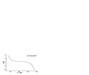
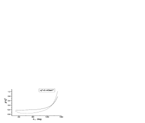
Figure 3: Charge asymmetry as a function of pion polar angle at fixed $q^{2}$ for $s=1$ GeV². Here the solid line corresponds to sQED, the dashed line – the full result in ChPT.

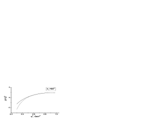
Figure 4: Charge asymmetry as a function of $q^{2}$ at fixed pion polar angle for $s=1$ GeV². Notation for the curves is the same as in Fig. 3.

In Figs. 3 and 4 we show the asymmetry dependence on pion polar angle (at fixed $q^{2}$) and on $q^{2}$ (at fixed pion polar angle). It follows from the calculations that the asymmetry changes sign at about $q^{2}=0.5$ GeV² (see Fig. 4). At all pion angles the difference between sQED and ChPT shows up only at small values of $q^{2}$, i.e at the high photon energies.

The sQED description is adequate for soft photon emission. It follows from Eqs. (31)–(34) that at small photon energies, $f_{1}^{sQED}\sim\frac{\mathstrut 1}{\omega}$,  $f_{2}^{sQED}\sim\frac{\mathstrut 1}{\omega^{2}}$, whereas $\Delta f_{i}$ which are responsible for the deviation from sQED behave rather as constants. Only at large photon energies the contribution from the intermediate $a_{1}$–meson (the last two diagrams in Fig. 2) can be sizable, because the denominators $D(l)D(-l)$ in Eqs. (32)–(34) approach the $a_{1}$–meson pole with the photon energy increasing.

For high value of $q^{2}$ the difference between predictions of sQED and full calculation in ChPT is small. For example, at $q^{2}=0.8$ GeV² and $q^{2}=0.6$ GeV² it is less than $1\%$ (the dashed and solid lines in Figs. 3 and 4 almost coincide). Taking into account that the asymmetry itself is less than $10^{-2}$, the experimental observation of such deviations in the energy region $q^{2}\geq 0.6$ GeV² is problematic.

Additional contribution coming from the process $\gamma^{*}\to\rho^{\pm}\pi^{\mp}\to\pi^{+}\pi^{-}\gamma$ turns out very small (see Appendix F) and does not change the above conclusion.

In order to test the calculation we can check that the asymmetry, integrated over the symmetric phase space of the pions, vanishes. Since no restriction has been imposed on the $\pi^{-}$ polar angle we impose no restriction on the $\pi^{+}$ polar angle, i.e. choose  $0^{\circ}\leq\theta_{+},\theta_{-}\leq 180^{\circ}$. Indeed, the integrated asymmetry is equal to zero.

4.2 Contribution from $e^{+}e^{-}\to\pi^{+}\pi^{-}\gamma$ to AMM of the muon

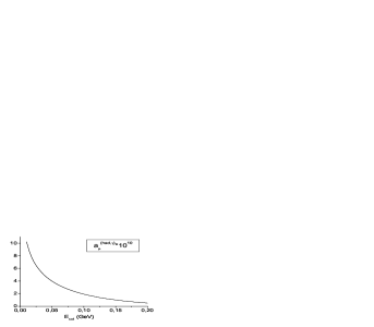
Figure 5: Differential contribution to $a_{\mu}^{(had,\gamma)}$ from $e^{+}e^{-}\to\pi^{+}\pi^{-}\gamma$, where $\gamma$ is the hard photon with energy $\omega\geq E_{cut}$ (left panel). Integrated contribution to $a_{\mu}^{(had,\gamma)}$ as a function of $E_{cut}$ for $s_{max}=1.5$ GeV² (right panel). The solid (dashed) line corresponds to the sQED (full) result.

Now we apply the previous results to the calculation of $a_{\mu}^{had,\gamma}$ which arises from the $\pi^{+}\pi^{-}\gamma$ channel. We should mention that only the radiation of the hard photon with the energy $\omega\geq E_{cut}$ is taken into account.

According to [20] $a_{\mu}^{had,\gamma}$ can be written in terms of the dispersion integral

$$a_{\mu}^{had,\gamma}=\frac{\alpha^{2}}{3\pi^{2}}\int_{4m_{\pi}^{2}}^{\infty}R^{\gamma}(s)K(s)\frac{\mathrm{d}s}{s},\;\;\;\;\;\;\;R^{\gamma}(s)=\frac{\sigma^{\pi^{+}\pi^{-},\gamma}(s)}{\sigma^{\mu^{+}\mu^{-}}(s)},$$ (40)

$$\sigma^{\mu^{+}\mu^{-}}(s)=\frac{4\pi\alpha^{2}}{3s}\Bigl{(}1+\frac{2m_{\mu}^{2}}{s}\Bigr{)}\sqrt{1-\frac{4m_{\mu}^{2}}{s}},$$

$$K(s)=\int_{0}^{1}\frac{x^{2}(1-x)}{x^{2}+(1-x)s/m_{\mu}^{2}}\mathrm{d}x,$$

where $m_{\mu}$ is the muon mass.

To obtain the cross section $\sigma^{\pi^{+}\pi^{-},\gamma}(s)$ we have to integrate Eq. (23) over $q^{2}$ from $4m_{\pi}^{2}$ to $q^{2}_{max}$. The value of $q^{2}_{max}$ is determined from the equality $q^{2}_{max}=s-2\sqrt{s}E_{cut}$. From the condition $q^{2}_{max}\geq 4m_{\pi}^{2}$, the lower limit of the integration in Eq. (40) is found to be $s_{min}=(E_{cut}+\sqrt{4m_{\pi}^{2}+E_{cut}^{2}})^{2}$. The upper limit in (40) is replaced by a finite $s_{max}$. The value of $s_{max}$ is chosen $s_{max}=1.5$ GeV², which is about of $O(m_{a_{1}}^{2})$, the upper limit of the applicability of ChPT with $\rho$ and $a_{1}$ mesons. The dependence of $a_{\mu}^{had,\gamma}$ on energy $E_{cut}$ is shown in Fig. 5.

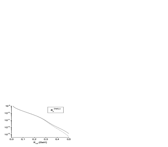
Figure 6: Integrated contribution to $a_{\mu}^{(had,\gamma)}$ as a function of $E_{cut}$ for $s_{max}=1.5$ GeV². Notation for the curves is the same as in Fig. 3.

As follows from our calculations the additional contributions to $a_{\mu}^{had,\gamma}$ stemming from ChPT are very small compared to the sQED result. This is in line with the conclusion of Ref. [21]. Even for relatively large cut-off energy $E_{cut}=200$ MeV the full result in ChPT differs from the sQED result only by $3.5\%$. For that reason the solid and dashed lines in Fig. 5 almost coincide. At the same time with increasing photon energy sQED begins to loose its predictive power. This is demonstrated in Fig. 6. In this region of energies the contribution from the $a_{1}$–meson is considerable and has to be taken into account. For example, at a photon energy about 500 MeV the deviation from sQED reaches $60\%$. However such a deviation (which is of the order of $10^{-12}$) is beyond the accuracy of the present measurements of the muon AMM.

5 Conclusions

In this article the FSR of a hard photon in the $e^{+}e^{-}\to\pi^{+}\pi^{-}\gamma$ reaction has been considered in framework of ChPT with vector $\rho$ and axial–vector $a_{1}$ mesons. The respective Lagrangian generates effective $\mathcal{O}(p^{4})$ chiral terms and, as substantiated in [14], is adequate for description of processes at energies up to about 1 GeV.

Our consideration of FSR is motivated by the necessity to study the model dependence of the hadronic contribution $a_{\mu}^{had,\gamma}$ to AMM of the muon. We have demonstrated that this dependence is weak, in particular, in the region of energies up to $s=1.5$ GeV² the differences between predictions of ChPT and sQED are very small compared to the present experimental accuracy. In general, the deviation of ChPT from sQED increases with increasing the minimal photon energy $E_{cut}$. However this deviation becomes essential only if the energy of the photon exceeds 400 MeV, in the region where $a_{\mu}^{had,\gamma}$ itself is beyond the existing experimental precision. To observe such effects the experimental accuracy has to be increased by at least one order of magnitude.

In fact, this small deviation is not surprising. Firstly, at fixed value of $s$ the low–energy photon region is described similarly in both models and, as follows from the calculation, this region dominates in $a_{\mu}^{had,\gamma}$. Secondly, the main contribution to the integral over $s$ in Eq. (40) comes from the region of the $\rho$–resonance, which is accounted for in the same way in sQED and ChPT through the VMD model. Therefore, the integral $a_{\mu}^{had,\gamma}$ is not sensitive to the chiral dynamics (see also discussion in [21]).

The developed approach has also allowed us to investigate the $C$–odd asymmetry of the cross section caused by the ISR – FSR interference. In general, measurements of the asymmetry can test the FSR amplitude. We considered radiation of the photon at the small angle relative to the direction of the electron momentum, $\theta<\theta_{0}=15^{\circ}$. In these conditions the absolute value of asymmetry is of the order of $\theta_{0}^{2}\sim 10^{-2}$. According to our calculations the difference between sQED and ChPT shows up only at the high photon energies $\omega\geq 0.3$ GeV. For the smaller photon energies the difference is less than $1\%$. Since the asymmetry itself is less than $10^{-2}$ for the selected collinear kinematics the experimental observation of this difference in the energy region $\omega<0.3$ GeV is problematic. Thus the model dependence of the asymmetry can experimentally be observed only at $q^{2}$ close to the threshold region, $4m_{\pi}^{2}\leq q^{2}<0.4$ GeV².

To our view, the photon FSR from the two–pion channel in $e^{+}e^{-}\to hadrons$ process shows the model dependence only near the two–pion threshold where the photon energy is large. In the bulk of energies (0.4 GeV${}^{2}<q^{2}<s$) scalar QED is sufficient to describe the FSR contribution to $a_{\mu}^{had,\gamma}$ and the $C$–odd asymmetry. In that way our results validate recent calculations [13] performed in framework of sQED.

It is plausible that the more complicated many–particle channels are more sensitive to the chiral dynamics.Another possibility to test chiral models is the region of the space-like photon momenta ($Q^{2}<0$). In particular, the virtual Compton scattering on the pion, $e^{-}\pi^{\pm}\to e^{-}\pi^{\pm}\gamma$, allows one to obtain information on the pion polarizabilities (see, e.g., [22, 16]).

Appendix A. General form of FSR tensor

The amplitude of the reaction $\gamma^{\ast}(Q)\rightarrow\gamma(k)+\pi^{+}(p_{+})+\pi^{-}(p_{-})$ depends on three 4-momenta, which can be chosen as $Q,k$, and $l\equiv p_{+}-p_{-}$. Here $Q=p_{1}+p_{2}$ is the total momentum of the $e^{+}e^{-}$ pair with $Q^{2}=s=4E^{2}$. For on-mass-shell pions $Q\cdot l=k\cdot l$. In general, the second-rank Lorentz tensor $M^{\mu\nu}(Q,k,l)$ can be decomposed through 10 independent tensors [23, 24]:

$$M^{\mu\nu}(Q,k,l)=\sum_{i=1}^{10}\Omega_{i}^{\mu\nu}F_{i}(Q^{2},k^{2},Q\cdot k,k\cdot l),$$ (A.1)

$$\Omega_{i}^{\mu\nu}=\{g^{\mu\nu},Q^{\mu}Q^{\nu},k^{\mu}k^{\nu},l^{\mu}l^{\nu},l^{\mu}Q^{\nu},Q^{\mu}l^{\nu},l^{\mu}k^{\nu},k^{\mu}l^{\nu},Q^{\mu}k^{\nu},k^{\mu}Q^{\nu}\},$$

where parity conservation is taken into account. The tensor $M^{\mu\nu}(Q,k,l)$ obeys the following properties:

$$M^{\mu\nu}(Q,k,l)=M^{\mu\nu}(Q,k,-l)=M^{\nu\mu}(-k,-Q,l).$$ (A.2)

The first equality follows from the charge conjugation symmetry of the S-matrix element $\langle\gamma(k),\pi^{+}(p_{+})\pi^{-}(p_{-})|S|\gamma^{\ast}(Q)\rangle=\langle\gamma(k),\pi^{-}(p_{+})\pi^{+}(p_{-})|S|\gamma^{\ast}(Q)\rangle$, and the second one is due to the photon crossing symmetry: $Q\leftrightarrow-k$ and $\mu\leftrightarrow\nu$.  Eqs. (A.2) impose certain constraints on the scalar functions $F_{i}(Q^{2},k^{2},Q\cdot k,k\cdot l)$.

The consideration below follows that of Ref. [24], where the virtual Compton scattering $\gamma^{\ast}(q)+\pi^{+}(p)\rightarrow\gamma(q^{\prime})+\pi^{+}(p^{\prime})$ with the space-like initial photon ($q^{2}<0$) and real final photon ($q^{\prime 2}=0$) has been studied in detail. Some of the results for the reaction $\gamma^{\ast}(Q)\rightarrow\gamma(k)+\pi^{+}(p_{+})+\pi^{-}(p_{-})$ can be obtained from the corresponding results of [24] after the substitutions: $p^{\mu}\rightarrow-p_{-}^{\mu}$, $p^{\prime\mu}\rightarrow p_{+}^{\mu}$, $q^{\mu}\rightarrow Q^{\mu}$, $q^{\prime\mu}\rightarrow k^{\mu}$.

The gauge invariance conditions $Q_{\mu}M^{\mu\nu}(Q,k,l)=0$ and $M^{\mu\nu}(Q,k,l)k_{\nu}=0$  lead to the five linear equations between functions the $F_{i}$ in Eq. (A.1), and in the general case of two virtual photons one is left with five scalar functions (see Eqs. (14) and (15) of [24]). We are interested in the situation, where the final photon is real, i.e. $k^{2}=0$ and $k^{\nu}\epsilon_{\nu}^{\prime}=0$ ($\epsilon_{\nu}^{\prime}$ is the polarization vector of the final photon), while the initial photon produced in $e^{+}e^{-}$ annihilation is virtual with $Q^{2}\geq 4m_{\pi}^{2}$. In this case one obtains

$$M^{\mu\nu}(Q,k,l)=-ie^{2}(\tau_{1}^{\mu\nu}f_{1}+\tau_{2}^{\mu\nu}f_{2}+\tau_{3}^{\mu\nu}f_{3})\equiv-ie^{2}M_{F}^{\mu\nu}(Q,k,l),$$ (A.3)

with the gauge invariant tensors

$$\tau_{1}^{\mu\nu} = k^{\mu}Q^{\nu}-g^{\mu\nu}k\cdot Q,$$

$$\tau_{2}^{\mu\nu} = k\cdot l(l^{\mu}Q^{\nu}-g^{\mu\nu}k\cdot l)+l^{\nu}(k^{\mu}k\cdot l-l^{\mu}k\cdot Q),$$

$$\tau_{3}^{\mu\nu} = Q^{2}(g^{\mu\nu}k\cdot l-k^{\mu}l^{\nu})+Q^{\mu}(l^{\nu}k\cdot Q-Q^{\nu}k\cdot l).$$ (A.4)

The scalar functions $f_{i}\equiv f_{i}(Q^{2},k\cdot Q,k\cdot l)$ are either even or odd with respect to the change of sign of the argument $k\cdot l$:

$$f_{1,2}(Q^{2},k\cdot Q,k\cdot l) = +f_{1,2}(Q^{2},k\cdot Q,-k\cdot l),$$

$$f_{3}(Q^{2},k\cdot Q,k\cdot l) = -f_{3}(Q^{2},k\cdot Q,-k\cdot l).$$ (A.5)

The factor $-ie^{2}$ in Eq. (A.3) is included for convenience. It thus follows that the evaluation of the FSR tensor amounts to the calculation of the scalar functions $f_{i}$  ($i=1,2,3$).

Appendix B. Chiral Lagrangian for pseudoscalar, vector and axial-vector mesons and photon

We choose the $\mathcal{O}(p^{2})$ chiral Lagrangian derived by Ecker et al. [14], which contains vector mesons and axial–vector mesons. It includes interaction of pseudoscalar, vector and axial–vector mesons, and photon. The explicit form is given in [14]:

$$L = \frac{f_{\pi}^{2}}{4}\mathrm{Tr}(D_{\mu}UD^{\mu}U^{\dagger}+\chi U^{\dagger}+\chi^{\dagger}U)-\frac{1}{4}F_{\mu\nu}F^{\mu\nu}$$ (B.1)

$$-\frac{1}{2}\mathrm{Tr}(\nabla^{\lambda}V_{\lambda\mu}\nabla_{\nu}V^{\nu\mu}-\frac{1}{2}m^{2}_{\rho}V_{\mu\nu}V^{\mu\nu})-\frac{1}{2}\mathrm{Tr}(\nabla^{\lambda}A_{\lambda\mu}\nabla_{\nu}A^{\nu\mu}-\frac{1}{2}m^{2}_{a}A_{\mu\nu}A^{\mu\nu})$$

$$+\frac{F_{V}}{2\sqrt{2}}\mathrm{Tr}(V_{\mu\nu}f_{+}^{\mu\nu})+\frac{iG_{V}}{\sqrt{2}}\mathrm{Tr}(V_{\mu\nu}u^{\mu}u^{\nu})+\frac{F_{A}}{2\sqrt{2}}\mathrm{Tr}(A_{\mu\nu}f_{-}^{\mu\nu}),$$

where $U=\exp(i\sqrt{2}\Phi/f_{\pi})$,  $\Phi$ describes the $SU(3)$ octet of pseudoscalar mesons, $V_{\mu\nu}\ (A_{\mu\nu})$ is antisymmetric field describing the $SU(3)$ octet of polar-vector (axial-vector) mesons, and $F^{\mu\nu}=\partial^{\mu}B^{\nu}-\partial^{\nu}B^{\mu}$ is the EM tensor, where the photon field is denoted by $B^{\mu}$. Further, $f_{\pi},\ F_{V},G_{V},F_{A}$ are constants, whose numerical values are specified in Sect. 4. For more details on definitions and notation see Ref. [14].

For treating the process $\gamma^{\ast}\rightarrow\pi^{+}\pi^{-}\gamma$ at tree level it is sufficient to keep in Eq. (B.1) the terms containing the neutral meson $\rho^{0}(770)$, and the charged mesons $a_{1}^{\pm}(1260)$ and $\pi^{\pm}$, as well as the photon. We obtain

$$L = ieB^{\mu}(\pi^{-}\partial_{\mu}\pi^{+}-\pi^{+}\partial_{\mu}\pi^{-})+e^{2}B_{\mu}B^{\mu}\pi^{+}\pi^{-}+e\frac{F_{V}}{2}F^{\mu\nu}\rho_{\mu\nu}^{0}(1-\frac{\pi^{+}\pi^{-}}{f_{\pi}^{2}})$$ (B.2)

$$+i\frac{G_{V}}{f_{\pi}^{2}}\rho_{\mu\nu}^{0}(\partial^{\mu}\pi^{+}\partial^{\nu}\pi^{-}-\partial^{\mu}\pi^{-}\partial^{\nu}\pi^{+})+ie\frac{F_{A}}{2f_{\pi}}F^{\mu\nu}(a_{1\mu\nu}^{+}\pi^{-}-a_{1\mu\nu}^{-}\pi^{+})$$

$$+e\frac{G_{V}}{f_{\pi}^{2}}\rho_{\mu\nu}^{0}[B^{\mu}(\pi^{+}\partial^{\nu}\pi^{-}+\pi^{-}\partial^{\nu}\pi^{+})-B^{\nu}(\pi^{+}\partial^{\mu}\pi^{-}+\pi^{-}\partial^{\mu}\pi^{+})].$$

Lagrangian (B.2) leads to the Feynman rules discussed in Appendix C. The diagrams contributing to the $\gamma^{\ast}\rightarrow\pi^{+}\pi^{-}\gamma$ reaction at tree level are shown in Fig. 2. For a general case of the two virtual photons we obtain the FSR tensor $M_{F}^{\mu\nu}$:

$$M_{F}^{\mu\nu} = \frac{1}{Q^{2}-2Q\cdot p_{-}}\Gamma^{\mu}(Q-p_{-},p_{-})\Gamma^{\nu}(p_{+},p_{+}+k)+(p_{+}\leftrightarrow p_{-})-2g^{\mu\nu}$$ (B.3)

$$+\frac{F_{V}^{2}-2F_{V}G_{V}}{f_{\pi}^{2}}\biggl{(}\frac{1}{m_{\rho}^{2}-Q^{2}}+\frac{1}{m_{\rho}^{2}-k^{2}}\biggr{)}(g^{\mu\nu}k\cdot Q-k^{\mu}Q^{\nu})$$

$$-\frac{2F_{V}G_{V}}{f_{\pi}^{2}}\left[\frac{1}{m_{\rho}^{2}-Q^{2}}(g^{\mu\nu}Q^{2}-Q^{\mu}Q^{\nu})+\frac{1}{m_{\rho}^{2}-k^{2}}(g^{\mu\nu}k^{2}-k^{\mu}k^{\nu})\right]$$

$$+\frac{F_{A}^{2}}{f_{\pi}^{2}m_{a}^{2}}\biggl{[}(g^{\mu\nu}k\cdot Q-k^{\mu}Q^{\nu})+\frac{1}{m_{a}^{2}-(Q-p_{-})^{2}}[(k+p_{+})^{\mu}(k\cdot Q(k+p_{+})^{\nu}$$

$$-k\cdot(k+p_{+}))-Q\cdot(k+p_{+})(k^{\mu}(k+p_{+})^{\nu}-k\cdot(k+p_{+})g^{\mu\nu})]+(p_{+}\leftrightarrow p_{-})\biggr{]}$$

where the EM vertex for the off-mass-shell pion (with initial $p_{i}$ and final $p_{f}$ momenta) is

$$\Gamma^{\mu}(p_{f},p_{i})=(p_{i}+p_{f})^{\mu}+\frac{F_{V}G_{V}}{f_{\pi}^{2}(m_{\rho}^{2}-r^{2})}[(p_{i}+p_{f})^{\mu}r^{2}-r^{\mu}(p_{f}^{2}-p_{i}^{2})],\;\;\;\;\;\;\;r\equiv p_{f}-p_{i}.$$ (B.4)

Note that Lagrangian (B.1) was applied in Ref. [16] in calculation of the Compton tensor for $\gamma^{\ast}\pi^{+}\rightarrow\gamma^{\ast}\pi^{+}$.

Appendix C. Feynman rules for ChPT Lagrangian

Following [14] we describe the vector (axial-vector) meson by the antisymmetric tensor field that corresponds to the following form of the propagator

$$i\Delta^{\alpha\beta;\mu\nu}(q)=\frac{i}{M^{2}(M^{2}-q^{2})}[g^{\alpha\mu}g^{\beta\nu}(M^{2}-q^{2})+g^{\alpha\mu}q^{\beta}q^{\nu}-g^{\alpha\nu}q^{\beta}q^{\mu}-(\alpha\leftrightarrow\beta)],$$ (C.1)

where $M$ is a mass of the vector (axial-vector) meson.

The vertices corresponding to the ChPT Lagrangian from Appendix B are listed in Fig. 7.

Figure 7:

Appendix D. Expressions for functions $h_{1,2}$

The functions $h_{1}$ and $h_{2}$ of Sect. 2.2 can be written as

$$h_{i}=h_{i}^{sQED}+\Delta h_{i},$$ (D.1)

where $h_{i}^{sQED}$ are determined from the following equations [11]

$$h_{2}^{sQED}(k\cdot q)^{2}=4\pi\xi|F_{\pi}(Q^{2})|^{2}[3q^{2}-(q^{2}+2m_{\pi}^{2})L_{1}]$$ (D.2)

$$2h_{1}^{sQED}-h_{2}^{sQED}Q^{2}=\frac{16\pi\xi|F_{\pi}(Q^{2})|^{2}}{(k\cdot Q)^{2}}[(k\cdot Q)^{2}+(\frac{Q^{2}}{4}-m_{\pi}^{2})(-q^{2}+(q^{2}-2m_{\pi}^{2})L_{1})]$$ (D.3)

with $\xi=\Bigl{(}1-\displaystyle\frac{\mathstrut 4m_{\pi}^{2}}{q^{2}}\Bigr{)}^{1/2}$ and $L_{1}=\displaystyle\frac{\mathstrut 1}{\xi}\ln\frac{1+\xi}{1-\xi}$.

From Eqs. (32)–(34) we obtain the equation for $\Delta h_{2}$ and $(2\Delta h_{1}-sh_{2})$ in ChPT

$$2\Delta h_{1}-s\Delta h_{2}=2\pi\xi\Biggl{\{}C_{1}+\frac{C_{2}L_{2}}{k\cdot Q}+\frac{C_{3}}{[(m_{a}^{2}-m_{\pi}^{2})(r-k\cdot Q)+\frac{4m_{\pi}^{2}(k\cdot Q)^{2}}{q^{2}}]}+4ReF_{\pi}(s)$$

$$\times\Biggl{[}fQ^{2}-ar+2m_{\pi}^{2}\Bigl{(}-f+a\frac{2(m_{a}^{2}-m_{\pi}^{2})(r-k\cdot Q)+2m_{\pi}^{2}r+k\cdot Q(m_{a}^{2}-m_{\pi}^{2})}{(m_{a}^{2}-m_{\pi}^{2})(r-k\cdot Q)}\Bigr{)}L_{1}$$

$$-\Biggl{(}\frac{4m_{\pi}^{2}(m_{a}^{2}+m_{\pi}^{2})(k\cdot Q)^{2}}{(m_{a}^{2}-m_{\pi}^{2})(r-k\cdot Q)}+2m_{\pi}^{2}q^{2}+(m_{a}^{2}-m_{\pi}^{2})(r+2Q^{2}-k\cdot Q)\Biggr{)}\frac{aL_{2}}{k\cdot Q}\Biggr{]}\Biggr{\}},$$ (D.4)

where

$$C_{1} = 2(k\cdot Q)^{2}f^{2}+af(2q^{2}k\cdot Q+rQ^{2})+\frac{1}{4}a^{2}((q^{2}-2k\cdot Q)q^{2}+2r^{2}),$$ (D.5)

$$C_{2} = -\frac{af}{2}\{(k\cdot Q)^{2}(Q^{2}+4k\cdot Q+4m_{\pi}^{2})+2k\cdot Q(Q^{2}+2k\cdot Q)r$$ (D.6)

$$+Q^{2}r^{2}\}+\frac{a^{2}}{8r}\{(k\cdot Q)^{2}[8m_{\pi}^{4}+2m_{\pi}^{2}(Q^{2}+6k\cdot Q)$$

$$+k\cdot Q(2Q^{2}+5k\cdot Q)]+2k\cdot Qr[-q^{2}Q^{2}+12k\cdot Q(m_{\pi}^{2}+k\cdot Q)]$$

$$-2r^{2}[Q^{4}+m_{\pi}^{2}q^{2}+k\cdot Q(Q^{2}-11k\cdot Q)]-4Q^{2}r^{3}-3r^{4}\},$$

$$C_{3} = \frac{a^{2}}{4}\{[8m_{\pi}^{4}+2m_{\pi}^{2}(-Q^{2}+6k\cdot Q)+5(k\cdot Q)^{2}+Q^{4}](k\cdot Q)^{2}+2rk\cdot Q$$ (D.7)

$$\times[Q^{4}+2Q^{2}k\cdot Q+4(k\cdot Q)^{2}+4m_{\pi}^{2}(k\cdot Q)]+r^{2}[Q^{4}+8Q^{2}k\cdot Q$$

$$+2(k\cdot Q)^{2}+2m_{\pi}^{2}q^{2}]+4Q^{2}r^{3}+r^{4}\},$$

$$\Delta h_{2}(k\cdot Q)^{2}=\frac{\pi a(m_{a}^{2}-m_{\pi}^{2})\xi}{2}\Biggl{\{}q^{2}(\frac{3a(m_{a}^{2}-m_{\pi}^{2})}{2}+8\mathrm{Re}F_{\pi}(s))+\frac{16(k\cdot Q)^{2}m_{\pi}^{2}ReF_{\pi}(s)}{(m_{a}^{2}-m_{\pi}^{2})(r-k\cdot Q)}L_{1}-$$

$$\Biggl{[}\frac{3q^{2}(m_{a}^{2}-m_{\pi}^{2})(r-k\cdot Q)+2(k\cdot Q)^{2}(q^{2}+2m_{\pi}^{2})}{4rk\cdot Q}a(m_{a}^{2}-m_{\pi}^{2})+$$

$$8ReF_{\pi}(s)\frac{r(q^{2}(m_{a}^{2}-m_{\pi}^{2})(r-k\cdot Q)+4(k\cdot Q)^{2}m_{\pi}^{2})}{2k\cdot Q(r-k\cdot Q)(m_{a}^{2}-m_{\pi}^{2})}\Biggr{]}L_{2}\Biggr{\}},$$ (D.8)

$$L_{2}=\frac{1}{\xi}\ln\frac{r+\xi k\cdot Q}{r-\xi k\cdot Q},\;\;\;\;\;\;r=m_{a}^{2}-m_{\pi}^{2}-k\cdot Q,$$

$$a=\frac{F_{A}^{2}}{m_{a}^{2}f_{\pi}^{2}},\;\;\;\;\;f=\frac{F_{V}^{2}-2F_{V}G_{V}}{f_{\pi}^{2}}\Biggl{(}\frac{1}{m_{\rho}^{2}}+\frac{1}{m_{\rho}^{2}-s-im_{\rho}\Gamma_{\rho}}\Biggr{)}.$$

Appendix E. Kinematics of the 3-particle final state

Solving energy-momentum conservation for the pion energy $E_{+}$ in Eq. (16) requires some care. Firstly, notice that the energy of the photon at fixed CM energy $\sqrt{s}=2E$ varies within the limits $0\leq\omega\leq\omega_{max}=E-m_{\pi}^{2}/E$. Secondly, by requiring positiveness of the expression under the square root in Eq. (16) at arbitrary $\cos\theta_{\gamma+}$, we get the conditions

$$\omega\leq\omega_{-}=\frac{2E(E-m_{\pi})}{2E-m_{\pi}},\;\;\;\;\;\;\;\omega\geq\omega_{+}=\frac{2E(E+m_{\pi})}{2E+m_{\pi}}.$$ (E.1)

Clearly $\omega_{+}\geq\omega_{max}$ and $\omega_{-}\leq\omega_{max}$. Thus the restriction for the photon energy is $0\leq\omega\leq\omega_{-}$. The corresponding invariant mass of the $\pi^{+}\pi^{-}$ pair is $4E^{2}\geq q^{2}\geq 4E^{2}m_{\pi}/(2E-m_{\pi})\approx 2Em_{\pi}$.

The requirement $0\leq\omega\leq\omega_{-}$ coincides with the condition that the energy conservation low in Eq. (14) leads to one solution for $E_{+}$, namely the one in Eq. (16). In the other case, if $\omega_{-}\leq\omega\leq\omega_{max}$, the situation becomes more complicated: there appear two solutions $E_{+}^{(-)}$ and $E_{+}^{(+)}$, which differ by the sign in front of the square root in Eq. (16). Correspondingly one has to sum over two terms in Eq. (14) corresponding to these solutions. Besides, the angle $\theta_{\gamma+}$ in this case is limited by the value

$$(\sin^{2}\theta_{\gamma+})_{max}=\frac{4E(E-\omega)[E(E-\omega)-m_{\pi}^{2}]}{m_{\pi}^{2}\omega^{2}}.$$ (E.2)

For these values of photon energies each angle $\theta_{\gamma+}$ in the Lab frame (CM frame for colliding $e^{+}e^{-}$ beams) corresponds to the two different angles between momenta of $\pi^{+}$ and $\gamma$ in the $\pi^{+}\pi^{-}$ CM frame. Here we refer to monograph [25] (ch. III), where these aspects of kinematics are considered in detail.

Appendix F. Contribution to FSR from $\rho^{\pm}\to\pi^{\pm}\gamma$ decays

The diagrams with intermediate charged $\rho$-meson can be obtained from the 3rd row of diagrams in Fig. 2, if $a_{1}^{\pm}$–meson is replaced by $\rho^{\pm}$–meson. We choose the chiral Lagrangian, describing the odd-intrinsic-parity sector, in the form [17]

$$L^{(V)}=H_{V}\epsilon_{\mu\nu\alpha\beta}\mathrm{Tr}(V^{\mu}\{u^{\nu},f_{+}^{\alpha\beta}\})\simeq-\frac{2\sqrt{2}eH_{V}}{3f_{\pi}}\epsilon_{\mu\nu\alpha\beta}F^{\alpha\beta}\vec{\rho}^{\mu}\partial^{\nu}{\vec{\pi}}$$ (F.1)

in the vector formulation for the $\rho$–meson field, where $\epsilon_{\mu\nu\alpha\beta}$ is the totally antisymmetric Levi-Civita tensor.

The constant $H_{V}$ can be determined from the $\rho^{\pm}\to\pi^{\pm}\gamma$ decay width $\Gamma(\rho^{\pm}\to\pi^{\pm}\gamma)=68.7$ keV [19]. From Eq. (F.1) one finds

$$\Gamma(\rho^{\pm}\to\pi^{\pm}\gamma)=\frac{4\alpha m_{\rho}^{3}H_{V}^{2}}{27f_{\pi}^{2}}(1-\frac{m_{\pi}^{2}}{m_{\rho}^{2}})^{3}$$ (F.2)

and thus $H_{V}=0.0363$.

The corresponding contribution to the invariant functions of Sect. 3 takes the form

$$\Delta f_{1}^{\rho^{\pm}} = \frac{8H_{V}^{2}}{9f_{\pi}^{2}}\biggl{[}({k\cdot Q+l^{2}})\biggl{(}\frac{1}{C(l)}+\frac{1}{C(-l)}\biggr{)}+2k\cdot l\biggl{(}\frac{1}{C(l)}-\frac{1}{C(-l)}\biggr{)}\biggr{]},$$ (F.3)

$$\Delta f_{2}^{\rho^{\pm}} = -\frac{8H_{V}^{2}}{9f_{\pi}^{2}}\biggl{(}\frac{1}{C(l)}+\frac{1}{C(-l)}\biggr{)},$$ (F.4)

$$\Delta f_{3}^{\rho^{\pm}} = \frac{8H_{V}^{2}}{9f_{\pi}^{2}}\biggl{(}\frac{1}{C(l)}-\frac{1}{C(-l)}\biggr{)},$$ (F.5)

where  $C(\pm l)=m_{\rho}^{2}-(k+p_{\pm})^{2}-im_{\rho}\Gamma_{\rho}((k+p_{\pm})^{2})$  with  $(k+p_{\pm})^{2}=(Q^{2}+l^{2}+2k\cdot Q\pm 4k\cdot l)/4$.

If we choose the antisymmetric–tensor field formulation for the $\rho$–meson as was done in the rest of this paper, then the Lagrangian, which is equivalent to (F.1) on the mass shell, reads

$$L^{(T)}=\frac{\sqrt{2}eH_{V}m_{\rho}}{3f_{\pi}}\epsilon_{\mu\nu\alpha\beta}F^{\alpha\beta}\vec{\rho}^{\mu\nu}\vec{\pi}.$$ (F.6)

For this Lagrangian the functions $\Delta f_{2,3}^{\rho^{\pm}}$ are the same as in (F.4) and (F.5), while $\Delta f_{1}^{\rho^{\pm}}$ differs from (F.3) by an additional term,

$$(\Delta f_{1}^{\rho^{\pm}})^{\prime}=\Delta f_{1}^{\rho^{\pm}}+\frac{64H_{V}^{2}}{9f_{\pi}^{2}}.$$ (F.7)

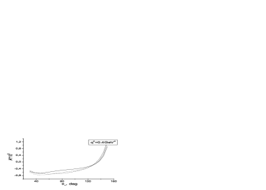
Figure 8: Charge asymmetry as a function of pion polar angle for $s=1$ GeV². The solid (dotted) line corresponds to the tensor (vector) formulation for $\rho$–meson, the dashed line – calculation without $\rho\to\pi\gamma$ contribution.

According to our calculations at invariant masses from the two–pion threshold to $q^{2}\approx 0.4$ GeV² the $\rho\to\pi\gamma$ contribution to the charge asymmetry may be of the same order as the $a_{1}\to\pi\gamma$ contribution, if the tensor formulation for the $\rho$–meson field is applied (see Fig. 8). For the higher values of $q^{2}$ the considered mechanism is suppressed with respect to other contributions.

Regarding the seeming difference between vector and tensor formulations, we should note that, as argued in [17, 26], the effective Lagrangians in the two formulations would become equivalent if the Lagrangian in the tensor formulation included an additional local term. Apparently the contribution from this local term to the functions $\Delta f_{i}^{\rho^{\pm}}$ would cancel the term $64H_{V}^{2}/(9f_{\pi}^{2})$ in (F.7) making the charge asymmetry independent of the formulation for the $\rho$–meson field. Therefore we can conclude that the contribution of the $\gamma^{*}\to\rho^{\pm}\pi^{\mp}\to\pi^{+}\pi^{-}\gamma$ process to the asymmetry is very small at all two–pion invariant masses.

References

• [1] S. Eidelman and F. Jegerlehner, Z. Phys. C 67, 585 (1995);
R. Alemany, M. Davier and A. Höcker, Eur. Phys. J. C 2, 123 (1998);
M. Davier, S. Eidelman, A. Höcker and Z. Zhang, Eur. Phys. J. C 27, 497 (2003) [arXiv: hep-ph/0208177].
• [2] R.M. Carey et al., Proposal of the BNL Experiment E969, 2004 (www.bnl.gov/henp/docs/pac0904/P969.pdf)
• [3] G. Cataldi, A.G. Denig, W. Kluge, S. Müller and G. Venanzoni, in Frascati 1999, Physics and detectors for DA$\Phi$NE, p. 569;
A. Aloisio et al., The KLOE Collaboration, arXiv: hep-ex/0107023;
A.G. Denig, The KLOE Collaboration, Nucl. Phys. B (Proc. Suppl.) 116, 243 (2003) [arXiv: hep-ex/0211024];
A. Aloisio et al., The KLOE Collaboration, arXiv: hep-ex/0312056;
A. Aloisio et al., The KLOE Collaboration, arXiv: hep-ex/0407048.
• [4] E.P. Solodov, The BaBar Collaboration, arXiv: hep-ex/0107027;
G.Sciolla, The BABAR Collaboration, Nucl. Phys. B (Proc. Suppl.) 99, 135 (2001) [arXiv: hep-ex/0101004];
N. Berger, arXiv: hep-ex/0209062.
• [5] M. Benayoun, S.I. Eidelman, V.N. Ivanchenko and Z.K. Silagadze, Mod. Phys. Lett. A 14, 2605 (1999).
• [6] Min-Shin Chen and P.M. Zerwas, Phys. Rev. D 11, 58 (1975).
• [7] A.B. Arbuzov, E.A. Kuraev, N.P. Merenkov and L. Trentadue, JHEP 12, 009 (1998);
M. Konchatnij and N.P. Merenkov, JETP Lett. 69, 811 (1999).
• [8] S. Binner, J.H. Kűhn, K. Melnikov, Phys. Lett. B 459, 279 (1999);
S. Spagnolo, Eur. Phys. J. C6, 637 (1999);
J. Kűhn, Nucl. Phys. B (Proc. Suppl.) 98, 2 (2001).
• [9] R.R. Akhmetshin et al., CMD-2 Collaboration, Phys. Lett. B 527, 161 (2002) [arXiv: hep-ex/0112031].
• [10] J.Z. Bai et al., BES Collaboration, Phys. Rev. Lett. 84, 594 (2000) [arXiv: hep–ex/0102003].
• [11] V.N. Baier and V.A. Khoze, Sov. Phys. JETP 21, 629 (1965); ibid., 21, 1145 (1965).
• [12] V.A. Khoze et al., Eur. Phys. J. C 25, 199 (2002).
• [13] H. Czyż, A. Grzelinska, J. Kűhn and G. Rodrigo, Eur. Phys. J. C 33, 333 (2004) [arXiv: hep-ph/0308312];
H. Czyż and A. Grzelinska, arXiv: hep-ph/0402030.
• [14] G. Ecker, J. Gasser, A. Pich and E. de Rafael, Nucl. Phys. B 321, 311 (1989);
G. Ecker, J. Gasser, H. Leutwyler, A. Pich and E. de Rafael, Phys. Lett. B 223, 425 (1989).
• [15] G. Ecker and R. Unterdorfer, Eur. Phys. J. C 24, 535 (2002) [arXiv: hep-ph/0203075].
• [16] J.F. Donoghue, B.R. Holstein and D. Wyler, Phys. Rev. D 47, 2089 (1993);
J.F. Donoghue and B.R. Holstein, Phys. Rev. D 48, 137 (1993).
• [17] G. Ecker, A. Pich and E. de Rafael, Phys. Lett. B 237, 481 (1990).
• [18] P.D. Ruiz-Femenía, A. Pich and J. Portolés, JHEP 0307, 003 (2003) [arXiv: hep-ph/0306157].
• [19] S. Eidelman et al. (Particle Data Group), Phys. Lett. B 592, 1 (2004)  (URL:  http://pdg.lbl.gov)
• [20] S.J. Brodsky and E. de Rafael, Phys. Rev. 68, 1620 (1968).
• [21] S.K. Dubinsky, A.Yu. Korchin and N.P. Merenkov, Zh. Eksp. Teor. Fiz. 126, 259 (2004) [arXiv: hep-ph/0407191]; JETP 99, 225 (2004).
• [22] C. Unkmeir, A. Ocherashvili, T. Fuchs, M.A. Moinester and S. Scherer, Phys. Rev. C 65, 015206 (2002) [arXiv: hep-ph/0107020].
• [23] R. Tarrach, Nuovo Cimento 28 A, 409 (1975).
• [24] D. Drechsel, G. Knöchlein, A. Metz and S. Scherer, Phys. Rev. C 55, 424 (1997) [arXiv: nucl-th/9608061].
• [25] E. Byckling and K. Kajantie. Particle kinematics. John Wiley and Sons, London - New York - Sydney - Toronto, 1973.
• [26] J. Bijnens and E. Pallante, Mod. Phys. Lett. A 11, 1069 (1996) [arXiv: hep-ph/9510338].