CERN-PH-TH/2004-216

TUM-HEP-561/04

MPP-2004-141

hep-ph/0410407

The $B\to\pi\pi,\pi K$ Puzzles in the Light of New Data:

Implications for the Standard Model,

New Physics and Rare Decays

Andrzej J. Buras,^a Robert Fleischer,^b Stefan Recksiegel^a and Felix Schwab^c,a

^a Physik Department, Technische Universität München, D-85748 Garching, Germany

^b Theory Division, Department of Physics, CERN, CH-1211 Geneva 23, Switzerland

^c Max-Planck-Institut für Physik – Werner-Heisenberg-Institut, D-80805 Munich, Germany

Recently, we developed a strategy to analyse the $B\to\pi\pi,\pi K$ data. We found that the $B\to\pi\pi$ measurements can be accommodated in the Standard Model (SM) through large non-factorizable effects. On the other hand, our analysis of the ratios $R_{\rm c}$ and $R_{\rm n}$ of the CP-averaged branching ratios of the charged and neutral $B\to\pi K$ modes, respectively, suggested new physics (NP) in the electroweak penguin sector, which may have a powerful interplay with rare decays. In this paper, we confront our strategy with recent experimental developments, addressing also the direct CP violation in $B_{d}\to\pi^{\mp}K^{\pm}$, which is now an established effect, the relation to its counterpart in $B^{\pm}\to\pi^{0}K^{\pm}$, and the first results for the direct CP asymmetry of $B_{d}\to\pi^{0}\pi^{0}$ that turn out to be in agreement with our prediction. We obtain hadronic $B\to\pi\pi,\pi K$ parameters which are almost unchanged and arrive at an allowed region for the unitarity triangle in perfect accordance with the SM. The “$B\to\pi K$ puzzle” persists, and can still be explained through NP, as in our previous analysis. In fact, the recently observed shifts in the experimental values of $R_{\rm c}$ and $R_{\rm n}$ have been predicted in our framework on the basis of constraints from rare decays. Conversely, we obtain a moderate deviation of the ratio $R$ of the CP-averaged $B_{d}\to\pi^{\mp}K^{\pm}$ and $B^{\pm}\to\pi^{\pm}K$ rates from the current experimental value. However, using the emerging signals for $B^{\pm}\to K^{\pm}K$ modes, this effect can be attributed to certain hadronic effects, which have a minor impact on $R_{\rm c}$ and do not at all affect $R_{\rm n}$. Our results for rare decays remain unchanged.

October 2004

1 Introduction

A particularly interesting aspect of the physics programme of the $B$ factories for the exploration of the Kobayashi–Maskawa mechanism of CP violation [1] is given by $B\to\pi\pi$ and $B\to\pi K$ modes (see [2, 3] and references therein). In the summer of 2003, the last missing element of the $B\to\pi\pi$ system, $B^{0}_{d}\to\pi^{0}\pi^{0}$, was eventually observed by the BaBar [4] and Belle collaborations [5], with a surprisingly prominent rate, pointing to large corrections to the predictions of the QCD factorization approach [6, 7]. Concerning the $B\to\pi K$ system, the last missing transition, $B^{0}_{d}\to\pi^{0}K^{0}$, was already observed by the CLEO collaboration in 2000 [8], and is now well established. Immediately after that measurement, a puzzling pattern in the ratios $R_{\rm c}$ and $R_{\rm n}$ of the charged and neutral $B\to\pi K$ rates has been pointed out [9]. This “$B\to\pi K$ puzzle” has survived over the years and was recently reconsidered by several authors (see, for instance, [7, 10, 11, 12]). It is an important feature of the observables $R_{\rm c}$ and $R_{\rm n}$ that they are significantly affected by (colour-allowed) electroweak (EW) penguins [13, 14]. On the other hand, the ratio $R$ of the CP-averaged $B_{d}\to\pi^{\mp}K^{\pm}$ and $B^{\pm}\to\pi^{\pm}K$ branching ratios, which is expected to be only marginally affected by (colour-suppressed) EW penguins, does not show an anomalous behaviour. Since EW penguins offer an attractive avenue for new physics (NP) to manifest itself [15, 16], the $B\to\pi K$ puzzle may indicate NP in the EW penguin sector. Should this actually be the case, also several rare $K$ and $B$ decays may show NP effects [12], thereby complementing the $B\to\pi K$ puzzle in a valuable manner.

In [17, 18], we developed a strategy to address these exciting issues systematically, with the following logical structure:

• Using the isospin flavour symmetry of strong interactions and assuming the range for the angle $\gamma$ of the unitarity triangle (UT) that follows in the Standard Model (SM) from the CKM fits [19, 20, 21], we may extract a set of hadronic parameters characterizing the $B\to\pi\pi$ system from the experimental results for the corresponding CP-averaged branching ratios and the CP-violating observables of $B_{d}\to\pi^{+}\pi^{-}$. We found large deviations of the hadronic parameters from the predictions of QCD factorization. Moreover, we could predict the CP asymmetries of the $B_{d}\to\pi^{0}\pi^{0}$ decay in the SM.

• If we use the $SU(3)$ flavour symmetry and neglect penguin annihilation and exchange topologies, which can be probed through $B_{d}\to K^{+}K^{-}$ and $B_{s}\to\pi^{+}\pi^{-}$ modes, the hadronic $B\to\pi\pi$ parameters allow us to determine their $B\to\pi K$ counterparts. Assuming again the SM, as in the $B\to\pi\pi$ analysis, we may predict all observables offered by the $B\to\pi K$ system, including also CP asymmetries. We found agreement with the experimental picture for $R$, whereas the situation in the $R_{\rm n}$–$R_{\rm c}$ plane was not in accordance with experiment. This discrepancy could be resolved through NP effects in the EW penguin sector, requiring a significant enhancement of the parameter $q$ measuring their strength relative to the tree contributions, and a NP phase $\phi$, which vanishes in the SM, around $-90^{\circ}$.

• Assuming a more specific (but popular) scenario [22]–[26], where NP enters the EW penguin sector through $Z^{0}$ penguins , we obtain an interesting interplay between the parameters $q$ and $\phi$ following from the resolution of the $B\to\pi K$ puzzle and several rare $B$ and $K$ decays. This allowed us to explore the impact of the data for $B\to X_{s}\mu^{+}\mu^{-}$ and $K_{\rm L}\to\pi^{0}e^{+}e^{-}$ processes, constraining the enhancement of $q$ to be smaller than that suggested by the $B\to\pi K$ data, thereby favouring a smaller value of $R_{\rm c}$ and a larger value of $R_{\rm n}$. In fact, this pattern has been confirmed to a large extent by the new data. Taking these constraints into account, there may still be prominent NP effects in the rare-decay sector, the most spectacular ones in $K_{\rm L}\to\pi^{0}\nu\bar{\nu}$ and $B_{s,d}\to\mu^{+}\mu^{-}$, exhibiting branching ratios that could be enhanced with respect to the SM by factors of ${\cal O}(10)$ and ${\cal O}(5)$, respectively.

In addition, we discussed the determination of $\gamma$ (and the other two UT angles $\alpha$ and $\beta$), where we obtained a result in agreement with the CKM fits [19, 20, 21], had a closer look at the $B_{s}$-meson decays $B_{s}\to K^{+}K^{-}$ and $B_{s}\to\pi^{\pm}K^{\mp}$, and performed a couple of consistency checks of the $SU(3)$ flavour symmetry, which did not indicate large corrections.

As there were several exciting experimental developments thanks to the BaBar and Belle collaborations since we wrote our original papers [17, 18], it is interesting to confront our strategy with the most recent data, although the picture is still far from being settled. The most important aspects are the following:

• Several new results for the $B\to\pi\pi$ and $B\to\pi K$ branching ratios [28]–[31].

• First results for the direct CP asymmetry of $B_{d}\to\pi^{0}\pi^{0}$ [30, 31].

• Updates for the CP-violating observables of $B_{d}\to\pi^{+}\pi^{-}$ [32, 33], as well as for the CP asymmetries of several $B\to\pi K$ modes [28, 30, 34, 35].

• Observation of direct CP violation in $B_{d}\to\pi^{\mp}K^{\pm}$ [36, 37], representing a new milestone in the exploration of CP violation. Some implications of this measurement have been discussed in [38] and [39], concerning the SM and supersymmetry, respectively.

• Observation of $B_{d}\to K^{0}\bar{K}^{0}$, i.e. of the first $b\to d$ penguin decay, and an emerging signal for its charged counterpart $B^{\pm}\to K^{\pm}K$ [29].

In our analysis, we will use the averages for these new results that were compiled by the “Heavy Flavour Averaging Group” (HFAG) [40], but also make a number of refinements and generalizations, in particular:

• We include the EW penguins of the $B\to\pi\pi$ system in our analysis. As anticipated in [18], this has a small impact on the numerics, but is a conceptual improvement.

• In view of the new $B\to\pi K$ data, we investigate the impact of certain hadronic effects, which can be constrained through the emerging experimental signal for $B^{\pm}\to K^{\pm}K$ decays.

The outline is as follows: in Section 2, we focus on the $B\to\pi\pi$ system and move on to the $B\to\pi K$ modes in Section 3. Finally, we summarize our conclusions in Section 4.

2 The $B\to\pi\pi$ System

2.1 Amplitudes

The starting point of our analysis of the $B\to\pi\pi$ decays is given by the amplitudes

$$\sqrt{2}A(B^{+}\to\pi^{+}\pi^{0}) = -[\tilde{T}+\tilde{C}]=-[T+C]$$ (2.1)

$$A(B^{0}_{d}\to\pi^{+}\pi^{-}) = -[\tilde{T}+P]$$ (2.2)

$$\sqrt{2}A(B^{0}_{d}\to\pi^{0}\pi^{0}) = -[\tilde{C}-P],$$ (2.3)

which satisfy the following well-known isospin relation [41]:

$$\sqrt{2}A(B^{+}\to\pi^{+}\pi^{0})=A(B^{0}_{d}\to\pi^{+}\pi^{-})+\sqrt{2}A(B^{0}_{d}\to\pi^{0}\pi^{0}).$$ (2.4)

The individual amplitudes of (2.1)–(2.3) can be expressed as

$$P = \lambda^{3}A({\cal P}_{t}-{\cal P}_{c})\equiv\lambda^{3}A{\cal P}_{tc}$$ (2.5)

$$\tilde{T} = \lambda^{3}AR_{b}e^{i\gamma}\left[{\cal T}-\left({\cal P}_{tu}-{\cal E}\right)\right]$$ (2.6)

$$\tilde{C} = \lambda^{3}AR_{b}e^{i\gamma}\left[{\cal C}+\left({\cal P}_{tu}-{\cal E}\right)\right],$$ (2.7)

where

$$\lambda\equiv|V_{us}|=0.2240\pm 0.0036,\quad A\equiv|V_{cb}|/\lambda^{2}=0.83\pm 0.02$$ (2.8)

are the usual parameters in the Wolfenstein expansion of the Cabibbo–Kobayashi–Maskawa (CKM) matrix [42, 43],

$$R_{b}\equiv\sqrt{\bar{\rho}^{2}+\bar{\eta}^{2}}=\left(1-\frac{\lambda^{2}}{2}\right)\frac{1}{\lambda}\left|\frac{V_{ub}}{V_{cb}}\right|=0.37\pm 0.04$$ (2.9)

measures one side of the UT, the ${\cal P}_{q}$ describe the strong amplitudes of QCD penguins with internal $q$-quark exchanges ($q\in\{t,c,u\}$), including annihilation and exchange penguins, while ${\cal T}$ and ${\cal C}$ are the strong amplitudes of colour-allowed and colour-suppressed tree-diagram-like topologies, respectively, and ${\cal E}$ denotes the strong amplitude of an exchange topology. The amplitudes $\tilde{T}$ and $\tilde{C}$ differ from

$$T=\lambda^{3}AR_{b}e^{i\gamma}{\cal T},\quad C=\lambda^{3}AR_{b}e^{i\gamma}{\cal C}$$ (2.10)

through the $({\cal P}_{tu}-{\cal E})$ pieces, which may play an important rôle [44]. Note that these terms contain also the “GIM penguins” with internal up-quark exchanges, whereas their “charming penguin” counterparts enter in $P$ through ${\cal P}_{c}$, as can be seen in (2.5) [44]–[47]. In order to characterize the dynamics of the $B\to\pi\pi$ system, it is convenient to introduce the following hadronic parameters:

$$xe^{i\Delta}\equiv\frac{\tilde{C}}{\tilde{T}}=\left|\frac{\tilde{C}}{\tilde{T}}\right|e^{i(\delta_{\tilde{C}}-\delta_{\tilde{T}})}=\frac{{\cal C}+\left({\cal P}_{tu}-{\cal E}\right)}{{\cal T}-\left({\cal P}_{tu}-{\cal E}\right)}$$ (2.11)

$$de^{i\theta}\equiv-\frac{P}{\tilde{T}}e^{i\gamma}=-\left|\frac{P}{\tilde{T}}\right|e^{i(\delta_{P}-\delta_{\tilde{T}})}=-\frac{1}{R_{b}}\left[\frac{{\cal P}_{tc}}{{\cal T}-\left({\cal P}_{tu}-{\cal E}\right)}\right],$$ (2.12)

where $\delta_{\tilde{C}}$, $\delta_{\tilde{T}}$ and $\delta_{P}$ denote the CP-conserving strong phases of $\tilde{C}$, $\tilde{T}$ and $P$.

In the $B\to\pi\pi$ system, the EW penguin contributions are expected to play a minor rôle [48, 49], and were therefore neglected in (2.1)–(2.3). However, applying the isospin flavour symmetry of strong interactions, they can be included [13, 50], yielding

$$\sqrt{2}A(B^{+}\to\pi^{+}\pi^{0}) = -|\tilde{T}|e^{i\delta_{\tilde{T}}}\left[1+xe^{i\Delta}\right]\left[e^{i\gamma}+\tilde{q}e^{-i\beta}\right]$$ (2.13)

$$A(B^{0}_{d}\to\pi^{+}\pi^{-}) = -|\tilde{T}|e^{i\delta_{\tilde{T}}}\left[e^{i\gamma}-de^{i\theta}\right]$$ (2.14)

$$\sqrt{2}A(B^{0}_{d}\to\pi^{0}\pi^{0}) = |P|e^{i\delta_{P}}\left[1+\frac{x}{d}e^{i\gamma}e^{i(\Delta-\theta)}+\tilde{q}\left(\frac{1+xe^{i\Delta}}{d}\right)e^{-i\theta}e^{-i\beta}\right],$$ (2.15)

where

$$\tilde{q}\equiv\left|\frac{P_{\rm EW}}{T+C}\right|\approx 1.3\times 10^{-2}\times\left|\frac{V_{td}}{V_{ub}}\right|=1.3\times 10^{-2}\times\left(1-\frac{\lambda^{2}}{2}\right)\left|\frac{\sin\gamma}{\sin\beta}\right|\approx 3\times 10^{-2}$$ (2.16)

measures the strength of the sum of the colour-allowed and colour-suppressed EW penguin contributions with respect to the sum of the colour-allowed and colour-suppressed tree-diagram-like contributions. It should be emphasized that (2.16) was derived for the SM. In contrast to our previous analysis [17, 18], we shall also include the EW penguin contributions in the numerical analysis performed below. Although their impact is actually small, this is a conceptual improvement. However, as soon as we consider NP in the EW penguin sector, the $B\to\pi\pi$ analysis does no longer fully separate from that of the $B\to\pi K$ system, i.e. items i) and ii) of Section 1 are no longer completely independent. However, their cross talk is actually very small.

2.2 Input Observables

Following [17, 18], we use the ratios

$$R_{+-}^{\pi\pi} \equiv 2\left[\frac{\mbox{BR}(B^{+}\to\pi^{+}\pi^{0})+\mbox{BR}(B^{-}\to\pi^{-}\pi^{0})}{\mbox{BR}(B_{d}^{0}\to\pi^{+}\pi^{-})+\mbox{BR}(\bar{B}_{d}^{0}\to\pi^{+}\pi^{-})}\right]\frac{\tau_{B^{0}_{d}}}{\tau_{B^{+}}}$$ (2.17)

$$R_{00}^{\pi\pi} \equiv 2\left[\frac{\mbox{BR}(B_{d}^{0}\to\pi^{0}\pi^{0})+\mbox{BR}(\bar{B}_{d}^{0}\to\pi^{0}\pi^{0})}{\mbox{BR}(B_{d}^{0}\to\pi^{+}\pi^{-})+\mbox{BR}(\bar{B}_{d}^{0}\to\pi^{+}\pi^{-})}\right]$$ (2.18)

of the CP-averaged $B\to\pi\pi$ branching ratios, and the CP-violating observables provided by the time-dependent rate asymmetry

$$\frac{\Gamma(B^{0}_{d}(t)\to\pi^{+}\pi^{-})-\Gamma(\bar{B}^{0}_{d}(t)\to\pi^{+}\pi^{-})}{\Gamma(B^{0}_{d}(t)\to\pi^{+}\pi^{-})+\Gamma(\bar{B}^{0}_{d}(t)\to\pi^{+}\pi^{-})}$$ (2.19)

$$={\cal A}_{\rm CP}^{\rm dir}(B_{d}\to\pi^{+}\pi^{-})\cos(\Delta M_{d}t)+{\cal A}_{\rm CP}^{\rm mix}(B_{d}\to\pi^{+}\pi^{-})\sin(\Delta M_{d}t)$$

as the input for our $B\to\pi\pi$ analysis. Concerning the former quantities, they can be written in the following generic form:

$$R_{+-}^{\pi\pi}=F_{1}(d,\theta,x,\Delta;\gamma),\quad R_{00}^{\pi\pi}=F_{2}(d,\theta,x,\Delta;\gamma).$$ (2.20)

On the other hand, the CP-violating $B_{d}\to\pi^{+}\pi^{-}$ observables involve, in addition to the angle $\gamma$ of the UT, only the hadronic parameters $(d,\theta)$; the mixing-induced CP asymmetry depends, furthermore, on the $B^{0}_{d}$–$\bar{B}^{0}_{d}$ mixing phase $\phi_{d}$, which equals $2\beta$ in the SM. Consequently, we may write

$${\cal A}_{\rm CP}^{\rm dir}(B_{d}\to\pi^{+}\pi^{-})=G_{1}(d,\theta;\gamma),\quad{\cal A}_{\rm CP}^{\rm mix}(B_{d}\to\pi^{+}\pi^{-})=G_{2}(d,\theta;\gamma,\phi_{d}).$$ (2.21)

Explicit expressions for the functions $F_{1,2}$ and $G_{1,2}$ can be found in [18].

Quantity	This work	Previous analysis
$\mbox{BR}(B^{\pm}\to\pi^{\pm}\pi^{0})/10^{-6}$	$5.5\pm 0.6$	$5.2\pm 0.8$
$\mbox{BR}(B_{d}\to\pi^{+}\pi^{-})/10^{-6}$	$4.6\pm 0.4$	$4.6\pm 0.4$
$\mbox{BR}(B_{d}\to\pi^{0}\pi^{0})/10^{-6}$	$1.51\pm 0.28$	$1.9\pm 0.5$
$R_{+-}^{\pi\pi}$	$2.20\pm 0.31$	$2.12\pm 0.37$
$R_{00}^{\pi\pi}$	$0.67\pm 0.14$	$0.83\pm 0.23$
${\cal A}_{\rm CP}^{\rm dir}(B_{d}\to\pi^{+}\pi^{-})$	$-0.37\pm 0.11$	$-0.38\pm 0.16$
${\cal A}_{\rm CP}^{\rm mix}(B_{d}\to\pi^{+}\pi^{-})$	$+0.61\pm 0.14$	$+0.58\pm 0.20$

Table 1: The current status of the $B\to\pi\pi$ input data for our strategy, with averages taken from [40], and comparison with the picture of our previous analysis [17, 18]. For the evaluation of $R_{+-}^{\pi\pi}$, we have used the life-time ratio $\tau_{B^{+}}/\tau_{B^{0}_{d}}=1.086\pm 0.017$ [51].

In Table 1, we have summarized the current experimental situation of the $B\to\pi\pi$ observables that serve as an input for our strategy, comparing also with the values that we used for our previous analysis. Concerning the CP-averaged $B\to\pi\pi$ branching ratios, the values obtained by the BaBar [30] and Belle [31] collaborations are in accordance with one another. On the other hand, the picture of the CP-violating $B_{d}\to\pi^{+}\pi^{-}$ observables is still not yet settled. The BaBar and Belle results are now given as follows:

$${\cal A}_{\rm CP}^{\rm dir}(B_{d}\to\pi^{+}\pi^{-})=\left\{\begin{array}[]{ll}-0.09\pm 0.15\pm 0.04&\mbox{(BaBar \cite[cite]{[\@@bibref{}{BaBar-CP-Bpipi}{}{}]}),}\\ -0.58\pm 0.15\pm 0.07&\mbox{(Belle \cite[cite]{[\@@bibref{}{Belle-CP-Bpipi}{}{}]}),}\end{array}\right.$$ (2.22)

$${\cal A}_{\rm CP}^{\rm mix}(B_{d}\to\pi^{+}\pi^{-})=\left\{\begin{array}[]{ll}+0.30\pm 0.17\pm 0.03&\mbox{(BaBar \cite[cite]{[\@@bibref{}{BaBar-CP-Bpipi}{}{}]}),}\\ +1.00\pm 0.21\pm 0.07&\mbox{(Belle \cite[cite]{[\@@bibref{}{Belle-CP-Bpipi}{}{}]}).}\end{array}\right.$$ (2.23)

While these data differ from the ones used in [17, 18], the averages that are relevant for us changed only marginally as seen in Table 1. Since their physical interpretation is in impressive accordance with the picture of the SM, as we will see below, we expect that the experimental results will stabilize around these numbers.

2.3 Extraction of the Hadronic Parameters

If we assume that $\gamma$ and $\phi_{d}$ are known, (2.20) and (2.21) allow us to convert the experimental results for $R_{+-}^{\pi\pi}$, $R_{00}^{\pi\pi}$ and ${\cal A}_{\rm CP}^{\rm dir}(B_{d}\to\pi^{+}\pi^{-})$, ${\cal A}_{\rm CP}^{\rm mix}(B_{d}\to\pi^{+}\pi^{-})$ into values of $(d,\theta)$ and $(x,\Delta)$. Using the most recent results for the mixing-induced CP violation of the “golden” decay $B_{d}\to J/\psi K_{\rm S}$ (and related channels) obtained by the BaBar [52] and Belle collaborations [53], which correspond to the following new world average [40]:

$$\sin\phi_{d}=0.725\pm 0.037,$$ (2.24)

we obtain

$$\phi_{d}=\left(46.5^{+3.2}_{-3.0}\right)^{\circ},$$ (2.25)

in excellent agreement with the picture of the SM [19], and with $\phi_{d}=\left(47\pm 4\right)^{\circ}$ used in [17, 18]. It should be noted that we have neglected a second allowed solution for $\phi_{d}$ around $133^{\circ}$ in (2.25), which was analysed in detail in [54, 55]. This possibility is now disfavoured by the data for CP violation in $B_{d}\to D^{(\ast)\pm}\pi^{\mp}$ decays [56], our previous $B\to\pi\pi,\pi K$ analysis [18], and the first direct experimental result of the BaBar collaboration for the sign of $\cos\phi_{d}$. The latter follows from the measurement of the CP-violating observables of the time-dependent $B^{0}_{d}\to J/\psi[\to\ell^{+}\ell^{-}]K^{\ast}[\to\pi^{0}K_{\rm S}]$ angular distribution [57, 20] (performing a similar analysis of the Belle data, it was, however, not possible to put constraints on the sign of $\cos\phi_{d}$ [58]). Concerning $\gamma$, we assume the range

$$\gamma=(65\pm 7)^{\circ},$$ (2.26)

in accordance with the SM picture.

Parameter	EWPs included	EWPs neglected	Previous analysis
$d$	$0.51^{+0.26}_{-0.20}$	$0.51^{+0.26}_{-0.20}$	$0.48^{+0.35}_{-0.22}$
$\theta$	$\left(140^{+14}_{-18}\right)^{\circ}$	$\left(140^{+14}_{-18}\right)^{\circ}$	$+\left(138^{+19}_{-23}\right)^{\circ}$
$x$	$1.15^{+0.18}_{-0.16}$	$1.13^{+0.17}_{-0.16}$	$1.22^{+0.26}_{-0.21}$
$\Delta$	$-\left(59^{+19}_{-26}\right)^{\circ}$	$-\left(57^{+20}_{-30}\right)^{\circ}$	$-\left(71^{+19}_{-26}\right)^{\circ}$

Table 2: The hadronic parameters characterizing the $B\to\pi\pi$ system, extracted from the data summarized in Table 1 as explained in the text.

If we complement now the experimental results summarized in Table 1 with (2.25) and (2.26), we obtain the values of the hadronic parameters collected in Table 2. In the numbers of the “EWPs included” column, the EW penguins are taken into account through the SM expressions in (2.13)–(2.15), in contrast to the “EWPs neglected” column. For the purpose of comparison, we give also the results of our previous analysis [17, 18], where the EW penguin diagrams to the $B\to\pi\pi$ decays were neglected as well. We observe that the values of the hadronic parameters changed only marginally through the new data, and that the impact of the EW penguin topologies on the extraction of $(x,\Delta)$ is in fact small, as we anticipated. Note that the determination of $(d,\theta)$ is independent of the EW penguin effects.

As we discussed in terms of contours in the $\theta$–$d$ plane in [18], the extraction of $(d,\theta)$ from ${\cal A}_{\rm CP}^{\rm dir}(B_{d}\to\pi^{+}\pi^{-})$ and ${\cal A}_{\rm CP}^{\rm mix}(B_{d}\to\pi^{+}\pi^{-})$ is affected by a twofold discrete ambiguity. However, imposing, in addition, the information provided by $R_{+-}^{\pi\pi}$ and $R_{00}^{\pi\pi}$, we are only left with a single solution. A similar observation was subsequently also made by the authors of [59]. In Fig. 1, we show the corresponding $\chi^{2}$ plot for the determination of $d$ in order to illustrate this feature. For the resulting value of $(d,\theta)$, we obtain again a twofold solution for $(x,\Delta)$. However, this ambiguity can be resolved through the analysis of the $B\to\pi K$ system [18], yielding the solution listed in Table 2.

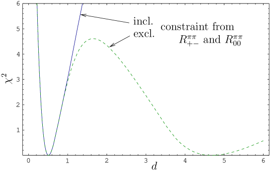
Figure 1: $\chi^{2}$ of a fit to ${\cal A}_{\rm CP}^{\rm dir}(B_{d}\to\pi^{+}\pi^{-})$ and ${\cal A}_{\rm CP}^{\rm mix}(B_{d}\to\pi^{+}\pi^{-})$ with (solid) and without (dashed) a simultaneous fit to $R_{+-}^{\pi\pi}$ and $R_{00}^{\pi\pi}$.

The extraction of the hadronic parameters $(d,\theta)$ and $(x,\Delta)$ discussed above relies only on the isospin flavour symmetry of strong interactions, takes isospin-breaking effects through EW penguin processes into account, and is essentially theoretically clean. Similar analyses were recently performed by several authors (see, for instance, [47, 59, 60, 61]), who confirmed the picture found in [17, 18]; the main differences between the various numerical results are due to the use of different input data.

The hadronic parameters in Table 2 allow us also to determine

$$\left[\frac{P}{T+C}\right]e^{i\gamma}=-\left[\frac{de^{i\theta}}{1+xe^{i\Delta}}\right]=\frac{1}{R_{b}}\left[\frac{{\cal P}_{tc}}{{\cal T}+{\cal C}}\right],$$ (2.27)

yielding

$$\left[\frac{P}{T+C}\right]e^{i\gamma}=\left(0.27^{+0.10}_{-0.08}\right)\times e^{-i(8^{+18}_{-13})^{\circ}}.$$ (2.28)

The experimental range for $R_{b}$ in (2.9) implies then

$$\frac{{\cal P}_{tc}}{{\cal T}+{\cal C}}=\left(0.10^{+0.04}_{-0.03}\right)\times e^{-i(8^{+18}_{-13})^{\circ}}.$$ (2.29)

These values refer to the case, where the EW penguins are included as in the SM; in the case of NP in the EW penguin sector, (2.28) and (2.29) change in a negligible manner. For further discussions of these parameters, we refer the reader to [18, 62].

2.4 Theoretical Picture

It is instructive to compare Table 2 with theoretical predictions. Concerning the “QCD factorization approach” (QCDF) [6], the most recent analysis was performed in [63], where hadronic parameters $(r,\phi)$ were introduced, which are related to $(d,\theta)$ through

$$d=\frac{r}{R_{b}},\quad\theta=\phi-\pi.$$ (2.30)

Using now the reference prediction for $r$ and $\phi$ in QCDF given in [63], $r=0.107\pm 0.031$ and $\phi=\left(8.6\pm 14.3\right)^{\circ}$, as well as the value of $R_{b}$ in (2.9), we obtain

$$\left.d\right|_{\rm QCDF}=0.29\pm 0.09,\quad\left.\theta\right|_{\rm QCDF}=-\left(171.4\pm 14.3\right)^{\circ}.$$ (2.31)

On the other hand, the application of the “perturbative hard-scattering approach” (PQCD) [64] yields the following prediction [65]:

$$\left.d\right|_{\rm PQCD}=0.23^{+0.07}_{-0.05},\quad+139^{\circ}<\left.\theta\right|_{\rm PQCD}<+148^{\circ}.$$ (2.32)

We observe that the results for $d$ are in agreement with each other, but significantly smaller than the values given in Table 2. On the other hand, the PQCD picture for the strong phase $\theta$ is in accordance with the data, whereas QCDF favours a smaller phase with the opposite sign. For recent analyses using the framework of the “soft collinear effective theory” (SCET) [66], we refer the reader to [47, 67].

Consequently, the theoretical attempts to calculate $d$ and $\theta$ from first principles are not in accordance with the values following from the SM interpretation of the current experimental data. This feature is already a challenge for several years (for earlier discussions, see, for instance, [54, 68]), and is now complemented by the measurement of the $B_{d}\to\pi^{0}\pi^{0}$ channel with a rate that is significantly larger than the one favoured in QCD factorization [7]. Unless the data will change in a dramatic manner, we have therefore to deal with large non-factorizable effects. This conclusion is in agreement with our previous one [17, 18], and the conclusions drawn in [47, 59, 60].

2.5 Prediction of the CP-Violating $B_{d}\to\pi^{0}\pi^{0}$ Observables

Having the hadronic parameters $(d,\theta)$ and $(x,\Delta)$ at hand, we may predict the CP-violating observables of the decay $B_{d}\to\pi^{0}\pi^{0}$, which take the following generic form:

$${\cal A}_{\rm CP}^{\rm dir}(B_{d}\to\pi^{0}\pi^{0})=H_{1}(d,\theta,x,\Delta;\gamma),\quad{\cal A}_{\rm CP}^{\rm mix}(B_{d}\to\pi^{0}\pi^{0})=H_{2}(d,\theta,x,\Delta;\gamma,\phi_{d});$$ (2.33)

explicit expressions can be found in [18]. The conceptual improvement with respect to our previous analysis is that we take again the EW penguin contributions into account. Complementing the values in Table 2 with (2.25) and (2.26), we obtain the SM predictions

$$\left.{\cal A}_{\rm CP}^{\rm dir}(B_{d}\to\pi^{0}\pi^{0})\right|_{\rm SM} = -0.28^{+0.37}_{-0.21}\,,$$ (2.34)

$$\left.{\cal A}_{\rm CP}^{\rm mix}(B_{d}\to\pi^{0}\pi^{0})\right|_{\rm SM} = -0.63^{+0.45}_{-0.41}\,,$$ (2.35)

which are in good agreement with our previous numbers, ${\cal A}_{\rm CP}^{\rm dir}(B_{d}\to\pi^{0}\pi^{0})=-0.41^{+0.35}_{-0.17}$ and ${\cal A}_{\rm CP}^{\rm mix}(B_{d}\to\pi^{0}\pi^{0})=-0.55^{+0.43}_{-0.45}$. We may now confront (2.34) with the first experimental results for the direct CP violation in $B_{d}\to\pi^{0}\pi^{0}$ that were recently reported by the BaBar and Belle collaborations:

$${\cal A}_{\rm CP}^{\rm dir}(B_{d}\to\pi^{0}\pi^{0})=\left\{\begin{array}[]{ll}-\left(0.12\pm 0.56\pm 0.06\right)&\mbox{(BaBar \cite[cite]{[\@@bibref{}{BaBar-Bpi0pi0}{}{}]}),}\\ -\left(0.43\pm 0.51\,^{+0.17}_{-0.16}\right)&\mbox{(Belle \cite[cite]{[\@@bibref{}{Belle-Bpi0pi0-new}{}{}]}),}\end{array}\right.$$ (2.36)

yielding the average of

$${\cal A}_{\rm CP}^{\rm dir}(B_{d}\to\pi^{0}\pi^{0})=-(0.28\pm 0.39).$$ (2.37)

Although the current errors are still large, the agreement between (2.34) and (2.37) is very encouraging. We look forward to having more accurate data available. As we noted and illustrated in [18], the measurement of one of the CP-violating $B_{d}\to\pi^{0}\pi^{0}$ observables allows the determination of $\gamma$.

3 The $B\to\pi K$ System

3.1 Preliminaries

The $B\to\pi K$ system consists of the four decay modes $B^{0}_{d}\to\pi^{-}K^{+}$, $B^{+}\to\pi^{+}K^{0}$, $B^{+}\to\pi^{0}K^{+}$ and $B^{0}_{d}\to\pi^{0}K^{0}$, which are governed by QCD penguin processes [3]. A key difference between these transitions is due to EW penguin topologies: in the case of the former two channels, these may only contribute in colour-suppressed form and are hence expected to play a minor rôle, whereas EW penguins have a significant impact on the latter two transitions thanks to colour-allowed contributions. In Table 3, we have summarized the current experimental status of the CP-averaged $B\to\pi K$ branching ratios. Following [17, 18], it is possible to fix the hadronic $B\to\pi K$ parameters through their $B\to\pi\pi$ counterparts $(d,\theta)$ and $(x,\Delta)$. To this end, we have to use the following working hypothesis:

• $SU(3)$ flavour symmetry of strong interactions.

• Neglect of penguin annihilation and exchange topologies.

Concerning i), we include the factorizable $SU(3)$-breaking corrections and perform internal consistency checks to probe non-factorizable $SU(3)$-breaking effects; the current data do not indicate large corrections of this kind. Assumption ii) can be tested with the help of $B_{d}\to K^{+}K^{-}$ and $B_{s}\to\pi^{+}\pi^{-}$ decays, where the current experimental $B$-factory bounds for the former channel do not indicate any anomalous behaviour. In particular at LHCb, where also $B_{s}\to\pi^{+}\pi^{-}$ will be accessible, it should be possible to explore the penguin annihilation and exchange topologies in a much more stringent manner.

Quantity	This work	Previous analysis
$\mbox{BR}(B_{d}\to\pi^{\mp}K^{\pm})/10^{-6}$	$18.2\pm 0.8$	$18.2\pm 0.8$
$\mbox{BR}(B^{\pm}\to\pi^{\pm}K)/10^{-6}$	$24.1\pm 1.3$	$21.8\pm 1.4$
$\mbox{BR}(B^{\pm}\to\pi^{0}K^{\pm})/10^{-6}$	$12.1\pm 0.8$	$12.5\pm 1.1$
$\mbox{BR}(B_{d}\to\pi^{0}K)/10^{-6}$	$11.5\pm 1.0$	$11.7\pm 1.4$
$R$	$0.82\pm 0.06$	$0.91\pm 0.07$
$R_{\rm c}$	$1.00\pm 0.08$	$1.17\pm 0.12$
$R_{\rm n}$	$0.79\pm 0.08$	$0.76\pm 0.10$

Table 3: The current status of the CP-averaged $B\to\pi K$ branching ratios, with averages taken from [40], and comparison with the picture of our previous analysis [17, 18]. For completeness, we give also the values of the ratios $R$, $R_{\rm c}$ and $R_{\rm n}$ introduced in (3.20), (3.42) and (3.43), where $R$ refers again to $\tau_{B^{+}}/\tau_{B^{0}_{d}}=1.086\pm 0.017$ [51].

3.2 Direct CP Violation in $B_{d}\to\pi^{\mp}K^{\pm}$

3.2.1 Experimental Picture

The most important new experimental development in the $B\to\pi K$ sector is the observation of direct CP violation in $B_{d}\to\pi^{\mp}K^{\pm}$ decays, which could eventually be established this summer by the BaBar [36] and Belle [37] collaborations. These measurements complement the observation of direct CP violation in the neutral kaon system by the NA48 (CERN) [69] and KTeV (FNAL) [70] collaborations, where this phenomenon is described by the famous observable $\mbox{Re}(\varepsilon^{\prime}/\varepsilon)$; the world average taking the final results of these experiments [71, 72] into account is given by $\mbox{Re}(\varepsilon^{\prime}/\varepsilon)=(16.6\pm 1.6)\times 10^{-4}$. For recent theoretical overviews of $\mbox{Re}(\varepsilon^{\prime}/\varepsilon)$, see [73, 74].

In the case of $B_{d}\to\pi^{\mp}K^{\pm}$, direct CP violation is characterized by the asymmetry

$${\cal A}_{\rm CP}^{\rm dir}(B_{d}\to\pi^{\mp}K^{\pm})\equiv\frac{\mbox{BR}(B^{0}_{d}\to\pi^{-}K^{+})-\mbox{BR}(\bar{B}^{0}_{d}\to\pi^{+}K^{-})}{\mbox{BR}(B^{0}_{d}\to\pi^{-}K^{+})+\mbox{BR}(\bar{B}^{0}_{d}\to\pi^{+}K^{-})},$$ (3.1)

which is now measured by the BaBar and Belle collaborations with the following results:

$${\cal A}_{\rm CP}^{\rm dir}(B_{d}\to\pi^{\mp}K^{\pm})=\left\{\begin{array}[]{ll}+0.133\pm 0.030\pm 0.009&\mbox{(BaBar \cite[cite]{[\@@bibref{}{BaBar-CP-dir-obs}{}{}]}),}\\ +0.101\pm 0.025\pm 0.005&\mbox{(Belle \cite[cite]{[\@@bibref{}{Belle-CP-dir-obs}{}{}]}).}\end{array}\right.$$ (3.2)

We observe that these numbers are nicely consistent with each other. They correspond to the following average [40]:

$${\cal A}_{\rm CP}^{\rm dir}(B_{d}\to\pi^{\mp}K^{\pm})=+0.113\pm 0.019,$$ (3.3)

establishing the direct CP violation in $B_{d}\to\pi^{\mp}K^{\pm}$ decays at the $5.9\sigma$ level.

3.2.2 Confrontation with Theory

Let us now follow the strategy developed in [17, 18] to confront the direct CP asymmetry of the $B_{d}^{0}\to\pi^{-}K^{+}$ channel with theoretical considerations. The corresponding decay amplitude can be written as

$$A(B^{0}_{d}\to\pi^{-}K^{+})=P^{\prime}\left[1-re^{i\delta}e^{i\gamma}\right],$$ (3.4)

with

$$P^{\prime}\equiv\left(1-\frac{\lambda^{2}}{2}\right)A\lambda^{2}({\cal P}_{t}^{\prime}-{\cal P}_{c}^{\prime})$$ (3.5)

and

$$re^{i\delta}\equiv\left(\frac{\lambda^{2}R_{b}}{1-\lambda^{2}}\right)\left[\frac{{\cal T}^{\prime}-({\cal P}_{t}^{\prime}-{\cal P}_{u}^{\prime})}{{\cal P}_{t}^{\prime}-{\cal P}_{c}^{\prime}}\right],$$ (3.6)

yielding

$${\cal A}_{\rm CP}^{\rm dir}(B_{d}\to\pi^{\mp}K^{\pm})=\frac{2r\sin\delta\sin\gamma}{1-2r\cos\delta\cos\gamma+r^{2}}.$$ (3.7)

The notation in (3.5) and (3.6) is analogous to that used for the discussion of the $B\to\pi\pi$ modes in Section 2; the primes remind us that we are dealing with $\bar{b}\to\bar{s}$ transitions. In (3.7), we can see nicely that ${\cal A}_{\rm CP}^{\rm dir}(B_{d}\to\pi^{\mp}K^{\pm})$ is induced through the interference between tree and QCD penguin topologies, with a CP-conserving strong phase difference $\delta$ and a CP-violating weak phase difference $\gamma$.

If we use now the working hypothesis given in Subsection 3.1, we obtain [17, 18]

$$re^{i\delta}=\frac{\epsilon}{d}e^{i(\pi-\theta)}.$$ (3.8)

This relation allows us to determine $(r,\delta)$ from the values of the hadronic $B\to\pi\pi$ parameters $(d,\theta)$ given in Table 2, with the following result:

$$r=0.10^{+0.05}_{-0.04},\quad\delta=+\left(39.6^{+17.7}_{-13.9}\right)^{\circ}.$$ (3.9)

Having these parameters at hand, which refer to the range for $\gamma$ in (2.26), we are in a position to calculate the direct CP asymmetry of $B_{d}\to\pi^{\mp}K^{\pm}$:

$${\cal A}_{\rm CP}^{\rm dir}(B_{d}\to\pi^{\mp}K^{\pm})=+0.127^{+0.102}_{-0.066},$$ (3.10)

which should be compared with our previous prediction of $+0.140^{+0.139}_{-0.087}$ [18]. Looking at (3.3), we observe that (3.10) is in nice agreement with the experimental result. In fact, in our previous analysis, which was confronted with the experimental average of ${\cal A}_{\rm CP}^{\rm dir}(B_{d}\to\pi^{\mp}K^{\pm})=+0.095\pm 0.028$, we advocated that this CP asymmetry should go up, in full accordance with the BaBar result in (3.2). Despite the large value of $\delta$, the rather small value of $r$ ensures that this CP asymmetry does not take a value that is much larger than the experimental ones.

In the case of QCDF [7, 75] and PQCD [65], the following patterns arise:

$$\left.{\cal A}_{\rm CP}^{\rm dir}(B_{d}\to\pi^{\mp}K^{\pm})\right|_{\rm QCDF}\sim-(0.05\pm 0.09),$$ (3.11)

$$+0.13\,\mathrel{\hbox{\hbox to0.0pt{\hbox{\lower 4.0pt\hbox{$\sim$}}\hss}\hbox{$<$}}}\,\left.{\cal A}_{\rm CP}^{\rm dir}(B_{d}\to\pi^{\mp}K^{\pm})\right|_{\rm PQCD}\,\mathrel{\hbox{\hbox to0.0pt{\hbox{\lower 4.0pt\hbox{$\sim$}}\hss}\hbox{$<$}}}\,+0.22.$$ (3.12)

Consequently, the QCDF picture is not in agreement with the experimental result (3.3), pointing in particular towards the opposite sign of the direct CP asymmetry. On the other hand, PQCD reproduces the sign correctly, but favours an asymmetry on the larger side. These features can also be seen with the help of (3.7) and (3.8) from the QCDF and PQCD predictions given in (2.31) and (2.32), respectively.

3.2.3 Alternative Confrontation with Theory

Another direct confrontation of ${\cal A}_{\rm CP}^{\rm dir}(B_{d}\to\pi^{\mp}K^{\pm})$ with theory is provided by the following SM relation, which can be derived with the help of assumptions i) and ii) specified in Subsection 3.1 [68, 76, 77]:

$$\epsilon H\equiv\underbrace{\left(\frac{f_{K}}{f_{\pi}}\right)^{2}\left[\frac{\mbox{BR}(B_{d}\to\pi^{+}\pi^{-})}{\mbox{BR}(B_{d}\to\pi^{\mp}K^{\pm})}\right]}_{\mbox{0.38$\pm$0.04}}=\underbrace{-\left[\frac{{\cal A}_{\rm CP}^{\rm dir}(B_{d}\to\pi^{\mp}K^{\pm})}{{\cal A}_{\rm CP}^{\rm dir}(B_{d}\to\pi^{+}\pi^{-})}\right]}_{\mbox{0.31$\pm$0.11}}.$$ (3.13)

Here, we have introduced the parameter

$$\epsilon\equiv\frac{\lambda^{2}}{1-\lambda^{2}}=0.053,$$ (3.14)

and the ratio $f_{K}/f_{\pi}=160/131$ of the kaon and pion decay constants takes the factorizable $SU(3)$-breaking corrections into account. In (3.13), we have also indicated the current experimental results, and observe that this relation is nicely satisfied within the current experimental uncertainties. This feature give us further confidence in our working assumptions, in addition to the agreement between (3.3) and (3.10).

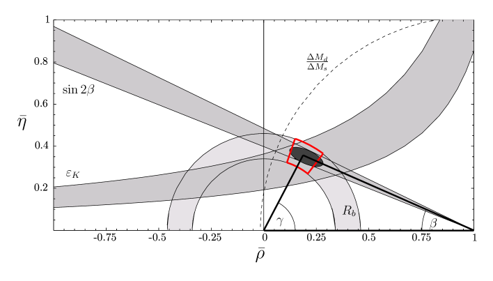
Figure 2: Illustration of the value of $\gamma$ following from the CP-violating $B_{d}\to\pi^{+}\pi^{-}$ observables and the data for the $B_{d}\to\pi^{\mp}K^{\pm}$ decays in the $\bar{\rho}$–$\bar{\eta}$ plane and comparison with the other constraints for the UT, as discussed in [78]. The shaded dark ellipse is the result of the UT fit, while the quadrangle corresponds to the second value of $\left.\gamma\right|_{\rm BR}$ in (3.17) and the $R_{b}$ constraint.

3.2.4 Implications for the UT

The quantity $H$ introduced in (3.13) can be written as follows:

$$H=G_{3}(d,\theta;\gamma).$$ (3.15)

If we now complement $H$ with the CP-violating observables ${\cal A}_{\rm CP}^{\rm dir}(B_{d}\to\pi^{+}\pi^{-})$ and ${\cal A}_{\rm CP}^{\rm mix}(B_{d}\to\pi^{+}\pi^{-})$, which take the general form in (2.21), and use the experimental result for $\phi_{d}$ in (2.25), we are in a position to determine $\gamma$ and $(d,\theta)$ [54, 55, 68, 77]. In addition to the expression involving the CP-averaged $B_{d}\to\pi^{+}\pi^{-}$ and $B_{d}\to\pi^{\mp}K^{\pm}$ branching ratios in (3.13), the corresponding direct CP asymmetries provide an alternative avenue for the determination of $H$, which is theoretically more favourable as far as the $SU(3)$-breaking corrections are concerned, but is currently affected by larger experimental uncertainties. The corresponding values of $H$ are given as follows:

$$\left.H\right|_{\rm BR}=7.2\pm 0.7,\quad\left.H\right|_{{\cal A}_{\rm CP}^{\rm dir}}=5.9\pm 2.1.$$ (3.16)

Complementing them with the CP-violating $B_{d}\to\pi^{+}\pi^{-}$ asymmetries in Table 1, we obtain the following solutions for $\gamma$:

$$\left.\gamma\right|_{\rm BR}=\left(39.6\,^{+5.8}_{-4.6}\right)^{\circ}\lor\left(63.3\,^{+7.7}_{-11.1}\right)^{\circ},\quad\left.\gamma\right|_{{\cal A}_{\rm CP}^{\rm dir}}=\left(38.1\,^{+5.4}_{-5.6}\right)^{\circ}\lor\left(66.6\,^{+11.0}_{-11.1}\right)^{\circ}.$$ (3.17)

As we discussed in [18], the twofold ambiguities arising in these determinations can be lifted by using additional experimental information for $B^{\pm}\to\pi^{\pm}K$ and the other $B\to\pi\pi$ decays, thereby leaving us with the values around $65^{\circ}$. In Fig. 2, we show the corresponding situation for the UT in the $\bar{\rho}$–$\bar{\eta}$ plane of the generalized Wolfenstein parameters [43], where we compare the values of $\gamma$ obtained above with the UT fit performed in [78]. Using, in addition, the range for the UT side $R_{b}$ in (2.9), we may also determine $\alpha$ and $\beta$, with the following results:

$$\left.\alpha\right|_{\rm BR}=\left(95.0\,^{+12.2}_{-8.2}\right)^{\circ},\quad\left.\alpha\right|_{{\cal A}_{\rm CP}^{\rm dir}}=\left(91.7\,^{+12.0}_{-11.0}\right)^{\circ},$$ (3.18)

$$\left.\beta\right|_{\rm BR}=\left(21.6\,^{+2.6}_{-2.7}\right)^{\circ},\quad\left.\beta\right|_{{\cal A}_{\rm CP}^{\rm dir}}=\left(21.7\,^{+2.5}_{-2.6}\right)^{\circ}.$$ (3.19)

The results for $\alpha$ are nicely consistent with those obtained from the most recent data for $B\to\rho\rho,\rho\pi$ processes, as reviewed in [79]; a similar comment applies to the ranges for $\gamma$ following from decays of the kind $B^{\pm}\to DK^{\pm}$. Let us also emphasize that our results for $\beta$ are in excellent agreement with the SM relation $\phi_{d}=2\beta$. In this context, it is important to stress that actually $\phi_{d}$ – and not $\beta$ itself – enters our analysis as an input parameter. The determination of $\alpha$ and $\beta$ in (3.18) and (3.19) is therefore an important test of the consistency of our approach (or of the SM relation $\phi_{d}=2\beta$).

More refined determinations of $\gamma$ from the CP-violating $B_{d}\to\pi^{+}\pi^{-}$ observables are provided by the decay $B_{s}\to K^{+}K^{-}$ [77]. This channel is already accessible at run II of the Tevatron [80, 81], and can be fully exploited at LHCb [82, 83]. In Appendix A, we collect the updated values of the SM predictions for the $B_{s}\to K^{+}K^{-}$ observables presented in [18].

3.3 The $B_{d}\to\pi^{\mp}K^{\pm}$, $B^{\pm}\to\pi^{\pm}K$ System

3.3.1 Experimental Picture

The direct CP violation in $B_{d}\to\pi^{\mp}K^{\pm}$ decays provides valuable information and is perfectly consistent with the SM picture emerging from our strategy [17, 18]. Let us now also consider the CP-averaged $B_{d}\to\pi^{\mp}K^{\pm}$ rate. In order to analyse this quantity, it is useful to consider simultaneously $B^{\pm}\to\pi^{\pm}K$ decays [49, 84, 85, 86], and to introduce

$$R\equiv\left[\frac{\mbox{BR}(B_{d}^{0}\to\pi^{-}K^{+})+\mbox{BR}(\bar{B}_{d}^{0}\to\pi^{+}K^{-})}{\mbox{BR}(B^{+}\to\pi^{+}K^{0})+\mbox{BR}(B^{-}\to\pi^{-}\bar{K}^{0})}\right]\frac{\tau_{B^{+}}}{\tau_{B^{0}_{d}}}.$$ (3.20)

The common feature of the $B^{0}_{d}\to\pi^{-}K^{+}$ and $B^{+}\to\pi^{+}K^{0}$ decays is that EW penguins may only contribute to them in colour-suppressed form, and are hence expected to play a minor rôle. As can be seen in Table 3, the experimental average for $R$ went down sizeably with respect to the situation of our previous analysis. This feature is essentially due to the most recent update of the CP-averaged $B^{\pm}\to\pi^{\pm}K$ branching ratio by the BaBar collaboration [29], taking certain radiative corrections into account; similar effects are currently investigated by the Belle collaboration [87]. Consequently, the experimental picture is not yet settled (see also [79]).

The last observable provided by the $B_{d}\to\pi^{\mp}K^{\pm}$, $B^{\pm}\to\pi^{\pm}K$ system is – in addition to ${\cal A}_{\rm CP}^{\rm dir}(B_{d}\to\pi^{\mp}K^{\pm})$ and $R$ – the direct CP asymmetry of the $B^{\pm}\to\pi^{\pm}K$ modes:

$${\cal A}_{\rm CP}^{\rm dir}(B^{\pm}\to\pi^{\pm}K)\equiv\frac{\mbox{BR}(B^{+}\to\pi^{+}K^{0})-\mbox{BR}(B^{-}\to\pi^{-}\bar{K}^{0})}{\mbox{BR}(B^{+}\to\pi^{+}K^{0})+\mbox{BR}(B^{-}\to\pi^{-}\bar{K}^{0})}.$$ (3.21)

The current experimental average is given as follows [40]:

$${\cal A}_{\rm CP}^{\rm dir}(B^{\pm}\to\pi^{\pm}K)=+0.020\pm 0.034,$$ (3.22)

and does not indicate any CP-violating effects in this channel.

3.3.2 Confrontation with Theory

In order to complement the $B^{0}_{d}\to\pi^{-}K^{+}$ amplitude in (3.4), we write

$$A(B^{+}\to\pi^{+}K^{0})=-P^{\prime}\left[1+\rho_{\rm c}e^{i\theta_{\rm c}}e^{i\gamma}\right],$$ (3.23)

where $P^{\prime}$ was defined in (3.5), and

$$\rho_{\rm c}e^{i\theta_{\rm c}}\equiv\left(\frac{\lambda^{2}R_{b}}{1-\lambda^{2}}\right)\left[\frac{{\cal P}_{t}^{\prime}-\tilde{\cal P}_{u}^{\prime}-{\cal A}^{\prime}}{{\cal P}_{t}^{\prime}-{\cal P}_{c}^{\prime}}\right].$$ (3.24)

Here $\tilde{\cal P}_{u}^{\prime}$ describes the penguins with internal up-quark exchanges contributing to the charged $B\to\pi K$ modes, and ${\cal A}^{\prime}$ is an annihilation topology. We arrive then straightforwardly at the following expression for $R$:

$$R=\frac{1-2r\cos\delta\cos\gamma+r^{2}}{1+2\rho_{\rm c}\cos\theta_{\rm c}\cos\gamma+\rho_{\rm c}^{2}},$$ (3.25)

while the direct CP asymmetry of the $B^{\pm}\to\pi^{\pm}K$ modes is given by

$${\cal A}_{\rm CP}^{\rm dir}(B^{\pm}\to\pi^{\pm}K)=-\left[\frac{2\rho_{\rm c}\sin\theta_{\rm c}\sin\gamma}{1+2\rho_{\rm c}\cos\theta_{\rm c}\cos\gamma+\rho_{\rm c}^{2}}\right].$$ (3.26)

Let us first assume that $\rho_{\rm c}$ can be neglected, as is usually done for the analysis of the $B_{d}\to\pi^{\mp}K^{\pm}$, $B^{\pm}\to\pi^{\pm}K$ system. This approximation corresponds to a vanishing value of (3.26), which is in accordance with (3.22). In view of the rather small experimental value of $R$, it is interesting (see also [79]) to return to the bounds on $\gamma$ that can be obtained with the help of

$$\sin^{2}\gamma\leq R,$$ (3.27)

provided $R$ is measured to be smaller than 1 [84]. Using the value of $R=0.82\pm 0.06$ in Table 3, we obtain the upper bound

$$\gamma\leq\left(64.9^{+4.8}_{-4.2}\right)^{\circ},$$ (3.28)

which is basically identical with the range for $\gamma$ in (2.26).

In analogy to the prediction in (3.10), the hadronic parameters in (3.9) allow us also to calculate $R$, with the following result:

$$R=0.943^{+0.028}_{-0.021},$$ (3.29)

which is the update of $R=0.943^{+0.033}_{-0.026}$ given in [17, 18]. Comparing with the new experimental result in Table 3, we observe that it favours a smaller value. Consequently, in the case of $R$, we encounter now a sizeable deviation of our prediction from the experimental average, whereas we obtain excellent agreement with the $B$-factory data for the CP-violating $B_{d}\to\pi^{\mp}K^{\pm}$ asymmetry. Moreover, also the bound on $\gamma$ in (3.28) appears to be surprisingly close to the SM range. Since $R$ may be affected by $\rho_{\rm c}$, whereas ${\cal A}_{\rm CP}^{\rm dir}(B_{d}\to\pi^{\mp}K^{\pm})$ does not involve this hadronic parameter, it is therefore suggested that $\rho_{\rm c}$ has actually a non-negligible impact on the numerical analysis.

3.3.3 A Closer Look at $\rho_{\rm c}$

In addition to $R$, the parameter $\rho_{\rm c}$ enters also the direct CP asymmetry of the $B^{\pm}\to\pi^{\pm}K$ decays. It is interesting to illustrate these effects in the $R$–${\cal A}_{\rm CP}^{\rm dir}(B^{\pm}\!\to\!\pi^{\pm}K)$ plane. To this end, we use (3.25) with the central values of the hadronic parameters in (3.9), and (3.26) to calculate the contours for $\rho_{\rm c}=0.05$ and $0.10$ shown in Fig. 3. We observe that for $\rho_{\rm c}=0.05$ and $-30^{\circ}\leq\theta_{\rm c}\mathrel{\hbox{\hbox to0.0pt{\hbox{\lower 4.0pt\hbox{$\sim$}}\hss}\hbox{$<$}}}0^{\circ}$ the $1\sigma$ ranges of experiment and theory (the contours only show the central value) practically overlap, thereby resolving essentially the discrepancy between our theoretical prediction for $R$ and its most recent experimental value. Following Appendix D.3 of [18], we have also included a second error bar for our theoretical prediction that indicates the variation of $R$ if colour-suppressed EW penguins are taken into account at a rather prominent level of $a_{\rm C}^{(1)}=0.1$, with $\Delta_{\rm C}^{(1)}\in[0,360^{\circ}]$. We observe that, while the inclusion of these effects could also help to resolve the discrepancy, the impact of $\rho_{\rm c}$ is significantly more important.

After this encouraging observation, let us have a closer look at the status of $\rho_{\rm c}$. Access to this parameter is provided by the decay $B^{+}\to K^{+}\bar{K}^{0}$, which is related to $B^{+}\to\pi^{+}K^{0}$ through the interchange of all down and strange quarks, i.e. through the $U$-spin flavour symmetry of strong interactions [46, 88], which is a subgroup of $SU(3)_{\rm F}$. Applying this symmetry, we may write (for a detailed discussion, see [3])

$$K\equiv\left[\frac{1}{\epsilon R_{SU(3)}^{2}}\right]\left[\frac{\mbox{BR}(B^{\pm}\to\pi^{\pm}K)}{\mbox{BR}(B^{\pm}\to K^{\pm}K)}\right]=\frac{1+2\rho_{\rm c}\cos\theta_{\rm c}\cos\gamma+\rho_{\rm c}^{2}}{\epsilon^{2}-2\epsilon\rho_{\rm c}\cos\theta_{\rm c}\cos\gamma+\rho_{\rm c}^{2}},$$ (3.30)

where $R_{SU(3)}$ describes $SU(3)$-breaking corrections. In factorization, we obtain

$$R_{SU(3)}=\left[\frac{M_{B}^{2}-M_{\pi}^{2}}{M_{B}^{2}-M_{K}^{2}}\right]\left[\frac{F_{B\pi}(M_{K}^{2};0^{+})}{F_{BK}(M_{K}^{2};0^{+})}\right]=0.79,$$ (3.31)

where the numerical value refers to the recent light-cone sum-rule analysis performed in [89]. The measurement of $K$ allows us to obtain the following allowed range for $\rho_{\rm c}$:

$$\frac{1-\epsilon\sqrt{K}}{1+\sqrt{K}}\leq\rho_{\rm c}\leq\frac{1+\epsilon\sqrt{K}}{|1-\sqrt{K}|}.$$ (3.32)

Using the most recent upper bound of $\mbox{BR}(B^{\pm}\to K^{\pm}K)<2.35\times 10^{-6}$ (90% C.L.) reported by the BaBar collaboration [29], and the measured value of $\mbox{BR}(B^{\pm}\to\pi^{\pm}K)$ in Table 3, this relation implies

$$\rho_{\rm c}<0.13.$$ (3.33)

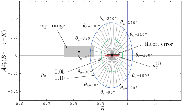
Figure 3: The situation in the $R$–${\cal A}_{\rm CP}^{\rm dir}(B^{\pm}\!\to\!\pi^{\pm}K)$ plane. We show contours for $\rho_{\rm c}=0.05$ and $\rho_{\rm c}=0.10$, with $\theta_{\rm c}\in[0^{\circ},360^{\circ}]$. The experimental ranges for $R$ and ${\cal A}_{\rm CP}^{\rm dir}(B^{\pm}\!\to\!\pi^{\pm}K)$ and our theoretical prediction are indicated in grey. The second error bar beneath the theoretical prediction (almost identical in size to the first one) indicates the variation of $R$ if colour-suppressed EW penguins are taken into account.

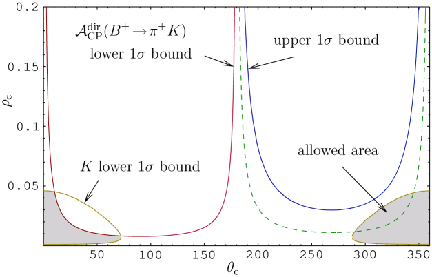
Figure 4: The constraints in the $\theta_{\rm c}$–$\rho_{\rm c}$ plane following from the current data for the CP-averaged $B^{\pm}\to K^{\pm}K$ branching ratio (parametrized by $K$) and the direct CP violation in $B^{\pm}\to\pi^{\pm}K$ decays as discussed in the text.

The neutral counterpart of $B^{+}\to K^{+}\bar{K}^{0}$, the $B^{0}_{d}\to K^{0}\bar{K}^{0}$ channel, was observed this summer by the BaBar collaboration [29], with the CP-averaged branching ratio

$$\mbox{BR}(B_{d}\to K^{0}\bar{K}^{0})=\left(1.19^{+0.40}_{-0.35}\pm 0.13\right)\times 10^{-6},$$ (3.34)

corresponding to a significance of $4.5\sigma$. This exciting measurement is the first direct experimental evidence for a $b\to d$ penguin process. Interestingly, it is in accordance with the lower SM bounds derived in [62], which suggested that the discovery of this transition should actually be just ahead of us. Concerning $B^{+}\to K^{+}\bar{K}^{0}$, there is an emerging signal at the $3.5\sigma$ level, which would correspond to

$$\mbox{BR}(B^{\pm}\to K^{\pm}K)=\left(1.45^{+0.53}_{-0.46}\pm 0.11\right)\times 10^{-6};$$ (3.35)

in the SM, we expect a lower bound of $(1.69^{+0.21}_{-0.24})\times 10^{-6}$ [90]. Inserting the range in (3.35) into (3.32) yields

$$-0.008\pm 0.008<\rho_{\rm c}<0.102\pm 0.009.$$ (3.36)

If we use the SM value of $\gamma$ in (2.26), the measurement of $\mbox{BR}(B^{\pm}\to K^{\pm}K)$ provides even more information. In fact, (3.30) allows us then to determine $\rho_{\rm c}$ as a function of $\theta_{\rm c}$ with the help of

$$\rho_{\rm c}=\tilde{a}\pm\sqrt{\tilde{a}^{2}-\tilde{b}},$$ (3.37)

where

$$\tilde{a}\equiv\left[\frac{\epsilon K+1}{K-1}\right]\cos\gamma\cos\theta_{\rm c},\quad\tilde{b}\equiv\frac{\epsilon^{2}K-1}{K-1}.$$ (3.38)

In analogy, the experimental result for ${\cal A}_{\rm CP}^{\rm dir}(B^{\pm}\to\pi^{\pm}K)$ allows us to fix another contour in the $\theta_{\rm c}$–$\rho_{\rm c}$ plane. Using (3.26), we obtain

$$\rho_{\rm c}=-\tilde{c}\pm\sqrt{\tilde{c}^{2}-1},$$ (3.39)

with

$$\tilde{c}=\left[1+\frac{\tan\gamma\tan\theta_{\rm c}}{{\cal A}_{\rm CP}^{\rm dir}(B^{\pm}\to\pi^{\pm}K)}\right]\cos\gamma\cos\theta_{\rm c}.$$ (3.40)

In Fig. 4, we assume $\gamma=65^{\circ}$, and confront these considerations with the experimental results in (3.22) and (3.35), despite the fact that the latter branching ratio corresponds only to an emerging signal for the $B^{\pm}\to K^{\pm}K$ channel. Since the corresponding lower $1\sigma$ and central values of $\mbox{BR}(B^{\pm}\to K^{\pm}K)$ would be smaller than the lower bound derived in [90], (3.37) would not have a physical solution for these results. However, for values of $\mbox{BR}(B^{\pm}\to K^{\pm}K)$ larger than this bound, we obtain an expanding allowed region in the $\theta_{\rm c}$–$\rho_{\rm c}$ plane, as shown in Fig. 4. We also observe that ${\cal A}_{\rm CP}^{\rm dir}(B^{\pm}\to\pi^{\pm}K)$ has a rather small impact on the overall allowed parameter space. It is interesting to note that the data favour strong phases $\theta_{\rm c}$ around $0^{\circ}$ (and not around $180^{\circ}$), as is suggested by the general expression in (3.24).

In the following, we will use $\rho_{\rm c}=0.05$ and $\theta_{\rm c}=0^{\circ}$, in agreement with (3.36) and the allowed region in Fig. 4; a more rigorous analysis will have to wait until the data for the $B^{\pm}\to K^{\pm}K$ decays will have improved. With these values and $\gamma=65^{\circ}$, we obtain

$$w_{\rm c}\equiv\sqrt{1+2\rho_{\rm c}\cos\theta_{\rm c}\cos\gamma+\rho_{\rm c}^{2}}=1.022\,.$$ (3.41)

As can be seen in (3.25), this quantity describes the impact of $(\rho_{\rm c},\theta_{\rm c})$ on $R$. In particular, the numerical value in (3.41) shifts the central value $R=0.943$ in (3.29) accordingly to 0.903. We observe that $R$ moves actually towards the experimental value through the impact of $\rho_{\rm c}$, thereby essentially resolving the discrepancy arising in Subsection 3.3.2.

To conclude the discussion of the $B_{d}\to\pi^{\mp}K^{\pm}$, $B^{\pm}\to\pi^{\pm}K$ system, let us emphasize that we can accommodate the corresponding data in the SM by using additional experimental information on $B^{\pm}\to K^{\pm}K$ decays, allowing us to take the hadronic parameter $\rho_{\rm c}$ into account. The remaining small numerical difference in the analysis of $R$, if confirmed by future data, could be due to (small) effects of colour-suppressed EW penguins, which enter $R$ as well [18, 86], and/or the limitations of our working hypothesis specified in Subsection 3.1. Moreover, we would also not be surprised to see the experimental value of $R$ moving up in the future.

3.4 The Charged and Neutral $B\to\pi K$ Systems

3.4.1 Experimental Picture

Let us now turn to the decays $B^{+}\to\pi^{0}K^{+}$ and $B^{0}_{d}\to\pi^{0}K^{0}$, where EW penguins enter in colour-allowed form. In order to analyse these transitions, it is particularly useful to introduce the following ratios:

$$R_{\rm c}\equiv 2\left[\frac{\mbox{BR}(B^{+}\to\pi^{0}K^{+})+\mbox{BR}(B^{-}\to\pi^{0}K^{-})}{\mbox{BR}(B^{+}\to\pi^{+}K^{0})+\mbox{BR}(B^{-}\to\pi^{-}\bar{K}^{0})}\right]$$ (3.42)

$$R_{\rm n}\equiv\frac{1}{2}\left[\frac{\mbox{BR}(B_{d}^{0}\to\pi^{-}K^{+})+\mbox{BR}(\bar{B}_{d}^{0}\to\pi^{+}K^{-})}{\mbox{BR}(B_{d}^{0}\to\pi^{0}K^{0})+\mbox{BR}(\bar{B}_{d}^{0}\to\pi^{0}\bar{K}^{0})}\right],$$ (3.43)

i.e. to consider separately the charged and neutral $B\to\pi K$ modes [13]. The experimental situation of these quantities is summarized in Table 3. We observe that $R_{\rm c}$ went down, thanks to the larger value of $\mbox{BR}(B^{\pm}\to\pi^{\pm}K)$, and that $R_{\rm n}$ moved marginally up.

Furthermore, the decay $B^{+}\to\pi^{0}K^{+}$ offers a direct CP asymmetry,

$${\cal A}_{\rm CP}^{\rm dir}(B^{\pm}\to\pi^{0}K^{\pm})\equiv\frac{\mbox{BR}(B^{+}\to\pi^{0}K^{+})-\mbox{BR}(B^{-}\to\pi^{0}K^{-})}{\mbox{BR}(B^{+}\to\pi^{0}K^{+})+\mbox{BR}(B^{-}\to\pi^{0}K^{-})}=-0.04\pm 0.04,$$ (3.44)

where we have also given the experimental average [40]. In the case of $B^{0}_{d}\to\pi^{0}K_{\rm S}$ decays, we have a final state with CP eigenvalue $-1$. Consequently, we may introduce a time-dependent rate asymmetry with the same structure as (2.19), exhibiting direct and mixing-induced CP asymmetries. The most recent values for these observables obtained by the BaBar [28] and Belle [35] collaborations are consistent with each other, and correspond to the following new averages [40]:

$${\cal A}_{\rm CP}^{\rm dir}(B_{d}\to\pi^{0}K_{\rm S}) = +0.09\pm 0.14$$ (3.45)

$${\cal A}_{\rm CP}^{\rm mix}(B_{d}\to\pi^{0}K_{\rm S}) = -(0.34^{+0.27}_{-0.29}).$$ (3.46)

3.4.2 Confrontation with Theory

The SM amplitudes for the decays $B^{0}_{d}\to\pi^{-}K^{+}$ and $B^{+}\to\pi^{+}K^{0}$ were already given in (3.4) and (3.23), respectively. In the case of the $B^{+}\to\pi^{0}K^{+}$ and $B^{0}_{d}\to\pi^{0}K^{0}$ modes, the decay amplitudes can be written in the following form within the SM:

$$\sqrt{2}A(B^{+}\to\pi^{0}K^{+}) = P^{\prime}\left[1+\rho_{\rm c}e^{i\theta_{\rm c}}e^{i\gamma}-\left(e^{i\gamma}-qe^{i\omega}\right)r_{\rm c}e^{i\delta_{\rm c}}\right]$$ (3.47)

$$\sqrt{2}A(B^{0}_{d}\to\pi^{0}K^{0}) = -P^{\prime}\left[1+\rho_{\rm n}e^{i\theta_{\rm n}}e^{i\gamma}-qe^{i\omega}r_{\rm c}e^{i\delta_{\rm c}}\right].$$ (3.48)

Here the parameter $q$, with the CP-conserving strong phase $\omega$, measures the importance of the EW penguins with respect to the tree-diagram-like topologies. In the SM, it can be determined with the help of the $SU(3)$ flavour symmetry of strong interactions [91], yielding

$$qe^{i\omega}=0.69\times\left[\frac{0.086}{|V_{ub}/V_{cb}|}\right];$$ (3.49)

for a detailed discussion of the colour-suppressed EW penguin contributions, which are neglected in (3.47) and (3.48), see Appendix D of [18]. Moreover, we have

$$r_{\rm c}e^{i\delta_{\rm c}}\equiv\left(\frac{\lambda^{2}R_{b}}{1-\lambda^{2}}\right)\left[\frac{{\cal T}^{\prime}+{\cal C}^{\prime}}{{\cal P}_{t}^{\prime}-{\cal P}_{c}^{\prime}}\right],$$ (3.50)

as well as

$$\rho_{\rm n}e^{i\theta_{\rm n}}\equiv\left(\frac{\lambda^{2}R_{b}}{1-\lambda^{2}}\right)\left[\frac{{\cal C}^{\prime}+({\cal P}_{t}^{\prime}-{\cal P}_{u}^{\prime})}{{\cal P}_{t}^{\prime}-{\cal P}_{c}^{\prime}}\right],$$ (3.51)

where the notation is analogous to the one introduced in Subsection 2.1; the primes remind us again that we have now turned to $\bar{b}\to\bar{s}$ modes. We observe that the hadronic parameters in (3.6), (3.50) and (3.51) satisfy the following relations:

$$r_{\rm c}e^{i\delta_{\rm c}}=re^{i\delta}+\rho_{\rm n}e^{i\theta_{\rm n}}$$ (3.52)

$$\rho_{\rm n}e^{i\theta_{\rm n}}=re^{i\delta}x^{\prime}e^{i\Delta^{\prime}},$$ (3.53)

with

$$x^{\prime}e^{i\Delta^{\prime}}\equiv\frac{{\cal C}^{\prime}+{\cal P}_{tu}^{\prime}}{{\cal T}^{\prime}-{\cal P}_{tu}^{\prime}}.$$ (3.54)

The values of $(r,\delta)$ following from the $B\to\pi\pi$ data can be found in (3.9). In analogy, we may use

$$x^{\prime}e^{i\Delta^{\prime}}=\left[\frac{f_{\pi}F_{BK}(M_{\pi}^{2};0^{+})}{f_{K}F_{B\pi}(M_{K}^{2};0^{+})}\right]xe^{i\Delta}$$ (3.55)

to determine $(x^{\prime},\Delta^{\prime})$ from their $B\to\pi\pi$ counterparts given in Table 2. The factor

$$\left[\frac{f_{\pi}F_{BK}(M_{\pi}^{2};0^{+})}{f_{K}F_{B\pi}(M_{K}^{2};0^{+})}\right]=1.05\pm 0.18,$$ (3.56)

where the numerical value refers to the light-cone sum-rule analysis of [89], describes factorizable $SU(3)$-breaking corrections. Since (3.8) is not affected by $SU(3)$-breaking effects within factorization, such a factor is not present in the case of this relation [77]. Finally, we obtain then, with the help of (3.53), the numerical values

$$\rho_{\rm n}=0.12^{+0.05}_{-0.05},\quad\theta_{\rm n}=-\left(19.6_{-23.7}^{+17.6}\right)^{\circ},$$ (3.57)

and (3.52) yields

$$r_{\rm c}=0.20^{+0.08}_{-0.06},\quad\delta_{\rm c}=\left(6.9^{+17.9}_{-13.4}\right)^{\circ}.$$ (3.58)

Alternatively, $r_{\rm c}$ can be determined through the following well-known relation [92]:

$$r_{\rm c}=\sqrt{2}\left|\frac{V_{us}}{V_{ud}}\right|\frac{f_{K}}{f_{\pi}}\sqrt{\frac{{\rm BR}(B^{\pm}\to\pi^{\pm}\pi^{0})}{{\rm BR}(B^{\pm}\to\pi^{\pm}K^{0})}}=0.190\pm 0.011,$$ (3.59)

which relies on the $SU(3)$ flavour symmetry and the neglect of the $\rho_{\rm c}$ term in (3.23).

Having the parameters in (3.57) and (3.58) at hand, we may predict the values of $R_{\rm c}$ and $R_{\rm n}$ and of the CP-violating observables of $B^{\pm}\to\pi^{\pm}K$, $B_{d}\to\pi^{0}K_{\rm S}$ in the SM with the help of the formulae given in [18]. In the case of the charged modes, we obtain

$$\left.R_{\rm c}\right|_{\rm SM}=1.14\pm 0.05\quad(1.12)\,,$$ (3.60)

$$\left.{\cal A}_{\rm CP}^{\rm dir}(B^{\pm}\to\pi^{0}K^{\pm})\right|_{\rm SM}=0.04\,^{+0.11}_{-0.08}\quad(0.04)\,,$$ (3.61)

where here (and in the following) the numbers with errors refer to $\rho_{\rm c}=0$, and the central value for the case $\rho_{\rm c}=0.05$, $\theta_{\rm c}=0^{\circ}$ is given in brackets. We observe that the impact of $\rho_{\rm c}$ on $R_{\rm c}$ is significantly weaker than in the case of $R$ discussed in Subsection 3.3.3. This is due to the feature that $\rho_{\rm c}$ enters $R$ already at ${\cal O}(\rho_{\rm c})$, whereas it affects $R_{\rm c}$ through second order terms of ${\cal O}(\rho_{\rm c}^{2})$ and ${\cal O}(\rho_{\rm c}r_{\rm c})$ [91]. On the other hand, $R_{\rm n}$ and the CP-violating observables of $B_{d}\to\pi^{0}K_{\rm S}$ are not affected by $\rho_{\rm c}$, so that we obtain the following SM predictions:

$$\left.R_{\rm n}\right|_{\rm SM}=1.11^{+0.04}_{-0.05}$$ (3.62)

$$\left.{\cal A}_{\rm CP}^{\rm dir}(B_{d}\to\pi^{0}K_{\rm S})\right|_{\rm SM}=0.07\,^{+0.08}_{-0.11},\quad\left.{\cal A}_{\rm CP}^{\rm mix}(B_{d}\to\pi^{0}K_{\rm S})\right|_{\rm SM}=-(0.87\pm 0.05).$$ (3.63)

So far, we could accommodate all features of the $B$-factory data for the $B\to\pi\pi$ and $B\to\pi K$ modes in a satisfactory manner in the SM. Now we observe that this is not the case for $R_{\rm n}$ and – to a smaller extend – for $R_{\rm c}$. As we have emphasized above, $R_{\rm n}$ does not depend on $\rho_{\rm c}$, so this parameter cannot be at the origin of this puzzle, in contrast to the case of $R$, and has, moreover, a minor impact on $R_{\rm c}$. Moreover, as we discussed in [18], the colour-suppressed EW penguin topologies have no impact on $R_{\rm n}$ in our SM analysis, as they can be absorbed in a certain manner, but could affect $R_{\rm c}$. However, as we have seen in Subsection 3.3.3, the analysis of $R$ disfavours anomalously large contributions of this kind, in contrast to the claims made in [20]. Concerning $SU(3)$-breaking corrections, the agreement between (3.3) and our SM prediction (3.10), the successful confrontation of (3.13) with the data, and the emerging picture of the UT – in perfect accordance with the SM – discussed in Subsection 3.2.4 do not indicate large corrections to (3.8). Moreover, the agreement between (3.58) and (3.59) indicates that the leading $SU(3)$-breaking effects are indeed described by the corresponding factors in (3.55) and (3.59). So what could then be the origin of the puzzling pattern of the measured values of $R_{\rm n}$ and $R_{\rm c}$?

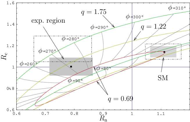
Figure 5: The situation in the $R_{\rm n}$–$R_{\rm c}$ plane. We show contours for values of $q=0.69$, $q=1.22$ and $q=1.75$, with $\phi\in[0^{\circ},360^{\circ}]$. The experimental ranges for $R_{\rm c}$ and $R_{\rm n}$ and those predicted in the SM are indicated in grey, the dashed lines serve as a reminder of the corresponding ranges in [18].

3.4.3 NP in the EW Penguin Sector

Since $R_{\rm n}$ and $R_{\rm c}$ are significantly affected by EW penguins, it is an attractive possibility to assume that NP enters through these topologies [15, 16]. In this case, the successful picture described above would not be disturbed. On the other hand, we may obtain full agreement between the theoretical values of $R_{\rm n}$ and $R_{\rm c}$ and the data. Following [17, 18], we generalize the EW penguin parameter as

$$q\to qe^{i\phi},$$ (3.64)

where $\phi$ is a CP-violating weak phase that vanishes in the SM, i.e. arises from NP. We may then use the measured values of $R_{\rm c}$ and $R_{\rm n}$ to determine $q$ and $\phi$, with the following results:

$$q=1.08\,^{+0.81}_{-0.73}\quad(1.23)\,,$$ (3.65)

$$\phi=-(88.8^{+13.7}_{-19.0})^{\circ}\quad(-86.8^{\circ})\,,$$ (3.66)

where the numbers in brackets illustrate again the impact of $\rho_{\rm c}=0.05$, $\theta_{\rm c}=0^{\circ}$ on the central values. Although these hadronic parameters are not at the origin of the $B\to\pi K$ puzzle, as we have seen above, they have of course some impact on the extracted values of $q$ and $\phi$, though the are not changing the overall picture.

It is useful to consider the $R_{\rm n}$–$R_{\rm c}$ plane, as we have done in Fig. 5. There we show contours corresponding to different values of $q$, and indicate the experimental and SM ranges. Following [18], we choose the values of $q=0.69$, $1.22$ and $1.75$, where the latter reproduced the central values of $R_{\rm c}$ and $R_{\rm n}$ in our previous analysis [17, 18]. The central values for the SM prediction have hardly moved, while their uncertainties have been reduced a bit. On the other hand, the central experimental values of $R_{\rm c}$ and $R_{\rm n}$ have moved in such a way that $q$ decreased, while the weak phase $\phi$ remains around $-90^{\circ}$.

Moreover, we obtain the following CP asymmetries in our NP scenario:

$${\cal A}_{\rm CP}^{\rm dir}(B^{\pm}\to\pi^{0}K^{\pm})=0.10^{+0.25}_{-0.19}\quad(0.10)$$ (3.67)

$${\cal A}_{\rm CP}^{\rm dir}(B_{d}\to\pi^{0}K_{\rm S})=0.01\,^{+0.15}_{-0.18},\quad{\cal A}_{\rm CP}^{\rm mix}(B_{d}\to\pi^{0}K_{\rm S})=-(0.98\,^{+0.02}_{-0.04}).$$ (3.68)

Although the central value of our prediction for ${\cal A}_{\rm CP}^{\rm dir}(B^{\pm}\to\pi^{0}K^{\pm})$ has a sign different from the corresponding experimental number, this cannot be considered as a problem because of the large current uncertainties. Concerning the observables of the $B_{d}\to\pi^{0}K_{\rm S}$ channel, our prediction for the direct CP asymmetry is rather close to the experimental number, while the current experimental result for mixing-induced asymmetry is somewhat on the lower side. However, the uncertainties of these very challenging measurements are still too large to draw conclusions.

Instead of using the value of $\omega=0^{\circ}$ in our analysis, which follows from the $SU(3)$ flavour symmetry, we could alternatively determine this strong phase, together with $q$ and $\phi$, from a combined analysis of $R_{\rm n}$, $R_{\rm c}$ and the direct CP asymmetry of the $B^{\pm}\to\pi^{0}K^{\pm}$ modes. In our previous analysis [18], this led to small values of $\omega$ in perfect agreement with the picture following from the $SU(3)$ flavour symmetry. Using the most recent data, we obtain

$$\omega=-\left(20\,^{+43}_{-28}\right)^{\circ},\quad q=1.08\,^{+0.82}_{-0.67},\quad\phi=-(88.2^{+14.0}_{-21.0})^{\circ}\,,$$ (3.69)

where the values of $q$ and $\phi$ are practically unchanged from the numbers given in (3.65) and (3.66), respectively. The updated value in (3.69) does still not favour dramatic $SU(3)$-breaking effects.

Finally, we would like to comment briefly on the direct CP asymmetry of the $B^{\pm}\to\pi^{0}K^{\pm}$ decays. It was argued in the recent literature (see, for instance, [79]) that the discrepancy between the experimental values in (3.3) and (3.44) was very puzzling. However, our analysis shows nicely that this is actually not the case. In particular, we have the following expression [18]:

$${\cal A}_{\rm CP}^{\rm dir}(B^{\pm}\to\pi^{0}K^{\pm})=\frac{2}{R_{\rm c}}\left[r_{\rm c}\sin\delta_{\rm c}\sin\gamma-qr_{\rm c}\left\{\sin(\delta_{\rm c}+\omega)\sin\phi+r_{\rm c}\sin\omega\sin(\gamma-\phi)\right\}\right],$$ (3.70)

where the $\rho_{\rm c}$ terms are neglected for simplicity. Consequently, the small value in (3.44) follows simply from the small strong phase $\delta_{\rm c}$ in (3.58). On the other hand, the hadronic parameters $r$ and $\delta$ governing ${\cal A}_{\rm CP}^{\rm dir}(B_{d}\to\pi^{\mp}K^{\pm})$ take very different values, as we have seen in Subsection 3.2.2. The difference between the CP-violating $B^{\pm}\to\pi^{0}K^{\pm}$ and $B_{d}\to\pi^{\mp}K^{\pm}$ asymmetries can therefore be straightforwardly explained through hadronic effects within the SM, i.e. does not require NP.

4 Conclusions

In this paper we have confronted our strategy for describing and correlating the $B\to\pi\pi$, $B\to\pi K$ decays and rare $K$ and $B$ decays with the new data on $B\to\pi\pi$, $B\to\pi K$ from BaBar and Belle. Within a simple NP scenario of enhanced CP-violating EW penguins considered by us, the NP contributions enter significantly only $B\to\pi K$ decays and rare $K$ and $B$ decays, while the $B\to\pi\pi$ system is practically unaffected by these contributions and can be described within the SM. Consequently the pattern of relations between various observables is in our strategy very transparent in that

• The relations between $B\to\pi\pi$ and $B\to\pi K$ decays are strictly connected with the long-distance physics allowing us to calculate the hadronic parameters of the $B\to\pi K$ from the $B\to\pi\pi$ ones without the intervention of NP contributions that enter at much shorter scales.

• The relations between $B\to\pi K$ decays and rare $K$ and $B$ decays are strictly connected with the short-distance physics allowing us to predict several spectacular departures from the SM expectations for rare $K$ and $B$ decays from the corresponding significant departures from the SM observed in the $B\to\pi K$ data.

The main messages from this new analysis are as follows:

• The present data for those observables in the $B\to\pi\pi$ and $B\to\pi K$ systems that are essentially unaffected by NP in the EW penguins are not only in accordance with our approach, but a number of predictions made by us in [17, 18] have been confirmed by the new data within theoretical and experimental uncertainties. This is in particular the case of the direct CP asymmetry in $B_{d}\to\pi^{\mp}K^{\pm}$ but also in $B_{d}\to\pi^{0}\pi^{0}$. For convenience of the reader, we collect all CP-violating quantities involved in our analysis in Table 4 and show the comparison of the experimental values with our predictions.

• The observed decrease of the ratio $R$ below our expectations in [17, 18] can be partially attributed to certain hadronic effects, represented by the non-vanishing value of $\rho_{\rm c}$, that could be tested in $B^{\pm}\to K^{\pm}K$ decays once these are experimentally better known. In particular the sign of $\rho_{\rm c}$, which is more solid than its magnitude, points towards the decrease of $R$ relative to our previous estimate. However, our present understanding of these effects allows us to expect that future more accurate measurements will find $R$ higher than its present central value.

• The decrease in the difference $R_{\rm c}-R_{\rm n}$ observed in the recent data of BaBar has been predicted by us on the basis of branching ratios for rare decays [17, 18]. This is explicitly seen in Table 2 of [18]. In this manner the overall description of $B\to\pi\pi$, $B\to\pi K$ and rare decays within our approach has improved with respect to our previous analysis.

• The picture of rare decays presented by us in [17, 18] remains unchanged, since the values of $q$ and $\phi$ obtained are still slightly above the bound from $b\to sl^{+}l^{-}$ used in [18]. In particular, the spectacular enhancement of $K_{\rm L}\to\pi^{0}\nu\bar{\nu}$ as well as the enhancement of several other rare decays remain. Further implications for rare decays in this scenario can be found in [93, 94]

• Last but certainly not least the obtained value of $\gamma$ and the UT are in full agreement with the usual CKM fits.

Finally, we would like to comment on analyses using only the $B\to\pi K$ data. It has been claimed in [20, 95, 96] that the puzzle concerning the $B\to\pi K$ system is significantly reduced or not even present. We would like to emphasize that a study of the $B\to\pi K$ decays alone is not very much constrained and consequently has a rather low resolution in search for NP effects. Such an analysis is moreover not satisfactory as it ignores the information on long distance dynamics that we have already from other non-leptonic decays, in particular from $B\to\pi\pi$ decays that are connected with the $B\to\pi K$ system through $SU(3)$ flavour symmetry. One should also not forget that, for a confrontation with the SM, the use of the $SU(3)$ flavour symmetry, which allows us to determine the EW penguin parameters $q$ and $\omega$ through (3.49), cannot be avoided. Consequently one may ask why the $SU(3)$ flavour symmetry should be used to find $q$ and not for getting the full input from $B\to\pi\pi$ and in the future from $B\to KK$ decays.

As demonstrated in [17, 18] and here, the use of the full information from the $B\to\pi\pi$ and $B\to\pi K$ systems allows us to uncover possible signals of NP effects in $B\to\pi K$ decays that in turn change significantly the SM pattern of rare decay branching ratios. In this respect, we disagree with a statement made in [79] that “the data seem to disfavour NP explanations, according to which NP primarily modifies electroweak penguin contributions”.

Quantity	Our Prediction	Experiment
${\cal A}_{\rm CP}^{\rm dir}(B_{d}\!\to\!\pi^{0}\pi^{0})$	$-0.28^{+0.37}_{-0.21}$	$-0.28\pm 0.39$
${\cal A}_{\rm CP}^{\rm mix}(B_{d}\!\to\!\pi^{0}\pi^{0})$	$-0.63^{+0.45}_{-0.41}$	$-0.48_{-0.40}^{+0.48}$
${\cal A}_{\rm CP}^{\rm dir}(B_{d}\!\to\!\pi^{\mp}K^{\pm})$	$0.127^{+0.102}_{-0.066}$	$0.113\pm 0.019$
${\cal A}_{\rm CP}^{\rm dir}(B^{\pm}\!\to\!\pi^{0}K^{\pm})$	$0.10^{+0.25}_{-0.19}$	$-0.04\pm 0.04$
${\cal A}_{\rm CP}^{\rm dir}(B_{d}\!\to\!\pi^{0}K_{\rm S})$	$0.01^{+0.15}_{-0.18}$	$0.09\pm 0.14$
${\cal A}_{\rm CP}^{\rm mix}(B_{d}\!\to\!\pi^{0}K_{\rm S})$	$-0.98^{+0.04}_{-0.02}$	$-0.34^{+0.29}_{-0.27}$

Table 4: Compilation of predictions for all CP-violating asymmetries in the $B\to\pi\pi$ and $B\to\pi K$ systems. We omit the quantities used as input.

It will be exciting to follow the experimental progress on $B\to\pi\pi$ and $B\to\pi K$ decays and the corresponding efforts in rare decays. In particular new messages from BaBar and Belle that the present central values of $R_{\rm c}$ and $R_{\rm n}$ have been confirmed at a high confidence level, a slight increase of $R$ and a message from KEK [97] in the next two years that the decay $K_{\rm L}\to\pi^{0}\nu\bar{\nu}$ has been observed would give a strong support to the NP scenario considered here.

Acknowledgments
The work presented here was supported in part by the German Bundesministerium für Bildung und Forschung under the contract 05HT4WOA/3 and the DFG Project Bu. 706/1-2.

Appendix A Predictions for the $B_{s}\to K^{+}K^{-}$ Observables

The decay $B_{s}\to K^{+}K^{-}$ is related to $B_{d}\to\pi^{+}\pi^{-}$ through the interchange of all down and strange quarks, i.e. through the $U$-spin flavour symmetry of strong interactions. Consequently, this symmetry allows us to determine the hadronic $B_{s}\to K^{+}K^{-}$ parameters $(d^{\prime},\theta^{\prime})$ through the values of their $B_{d}\to\pi^{+}\pi^{-}$ counterparts $(d,\theta)$ given in Table 2. Using then the range of $\gamma$ in (2.26), and the SM value $\phi_{s}=-2^{\circ}$ for the $B^{0}_{s}$–$\bar{B}^{0}_{s}$ mixing phase, we arrive at the following SM predictions, updating those given in [18]:

$${\cal A}_{\rm CP}^{\rm dir}(B_{s}\to K^{+}K^{-}) = 0.13^{+0.10}_{-0.07}$$ (A.1)

$${\cal A}_{\rm CP}^{\rm mix}(B_{s}\to K^{+}K^{-}) = -0.18\pm 0.05.$$ (A.2)

Concerning the CP-averaged $B_{s}\to K^{+}K^{-}$ branching ratio, which is of more immediate experimental interest, we have to take a certain $SU(3)$-breaking factor into account that has recently been calculated through QCD sum rules [98]. Following [18], we obtain the updated value

$$\mbox{BR}(B_{s}\to K^{+}K^{-})=(38^{+32}_{-23})\times 10^{-6}$$ (A.3)

from the $B\to\pi\pi$ data. Alternatively, we may calculate $\mbox{BR}(B_{s}\to K^{+}K^{-})$ with the help of the CP-averaged $B_{d}\to\pi^{\mp}K^{\pm}$ branching ratio, which requires, however, the additional assumption that penguin annihilation and exchange topologies play a minor rôle (see item ii in Subsection 3.1) . Following this avenue yields

$$\mbox{BR}(B_{s}\to K^{+}K^{-})=(35\pm 7)\times 10^{-6},$$ (A.4)

in nice agreement with (A.3). Let us note that the difference between (A.1)–(A.3) and the corresponding numbers in [18] is very small, whereas (A.4) did not change at all.

The CDF Collaboration has recently reported the first measurements of the CP-averaged $B_{s}\to K^{+}K^{-}$ branching ratio [81], corresponding to the preliminary result

$$\mbox{BR}(B_{s}\to K^{+}K^{-})=(34.3\pm 5.5\pm 5.2)\times 10^{-6}.$$ (A.5)

The agreement with our theoretical SM predictions is very impressive, giving further support to our strategy. We look forward to better data and hope that also first measurements of the CP-violating $B_{s}\to K^{+}K^{-}$ observables will be available in the near future. Here ${\cal A}_{\rm CP}^{\rm mix}(B_{s}\to K^{+}K^{-})$ would be particularly exciting, since this asymmetry may well be affected by NP contributions to $B^{0}_{s}$–$\bar{B}^{0}_{s}$ mixing, which would manifest themselves then as a discrepancy to (A.2). By the time this measurement will be available, the uncertainty of the SM prediction given there should be further reduced thanks to better $B_{d}\to\pi^{+}\pi^{-}$ input data.

References

- [1] M. Kobayashi and T. Maskawa, Prog. Theor. Phys. 49 (1973) 652.
- [2] The BaBar Physics Book, eds. P. Harrison and H.R. Quinn, SLAC-R-504 (1998).
- [3] R. Fleischer, Phys. Rep. 370 (2002) 537.
- [4] B. Aubert et al. [BaBar Collaboration], Phys. Rev. Lett. 91 (2003) 241801.
- [5] K. Abe et al. [Belle Collaboration], Phys. Rev. Lett. 91 (2003) 261801.
- [6] M. Beneke, G. Buchalla, M. Neubert and C.T. Sachrajda, Phys. Rev. Lett. 83 (1999) 1914.
- [7] M. Beneke and M. Neubert, Nucl. Phys. B675 (2003) 333.
- [8] D. Cronin-Hennessy et al. [CLEO Collaboration], Phys. Rev. Lett. 85 (2000) 515.
- [9] A.J. Buras and R. Fleischer, Eur. Phys. J. C16 (2000) 97.
- [10] T. Yoshikawa, Phys. Rev. D68 (2003) 054023.
- [11] M. Gronau and J.L. Rosner, Phys. Lett. B572 (2003) 43.
- [12] A.J. Buras, R. Fleischer, S. Recksiegel and F. Schwab, Eur. Phys. J. C32 (2003) 45.
- [13] A.J. Buras and R. Fleischer, Eur. Phys. J. C11 (1999) 93.
- [14] M. Neubert, JHEP 9902 (1999) 014.
- [15] R. Fleischer and T. Mannel, TTP-97-22 [hep-ph/9706261].
- [16] Y. Grossman, M. Neubert and A. Kagan, JHEP 9910 (1999) 029.
- [17] A.J. Buras, R. Fleischer, S. Recksiegel and F. Schwab, Phys. Rev. Lett. 92 (2004) 101804.
- [18] A.J. Buras, R. Fleischer, S. Recksiegel and F. Schwab, Nucl. Phys. B697 (2004) 133.
- [19] M. Battaglia et al., hep-ph/0304132.
- [20] J. Charles et al. [CKMfitter Group Collaboration], hep-ph/0406184.
- [21] M. Bona et al. [UTfit Collaboration], hep-ph/0408079.
- [22] G. Colangelo and G. Isidori, JHEP 9809 (1998) 009.
- [23] A.J. Buras and L. Silvestrini, Nucl. Phys. B546 (1999) 299.
- [24] A.J. Buras, A. Romanino and L. Silvestrini, Nucl. Phys. B520 (1998) 3.
- [25] A.J. Buras, G. Colangelo, G. Isidori, A. Romanino and L. Silvestrini, Nucl. Phys. B566 (2000) 3.
-
[26]
G. Buchalla, G. Hiller and G. Isidori,
Phys. Rev. D63 (2001) 014015;
D. Atwood and G. Hiller, LMU-09-03 [hep-ph/0307251]. - [27] V. Barger, C. W. Chiang, P. Langacker and H. S. Lee, Phys. Lett. B 598, 218 (2004)
- [28] B. Aubert et al. [BaBar Collaboration], BABAR-CONF-04/30 [hep-ex/0408062].
- [29] B. Aubert et al. [BaBar Collaboration], BABAR-CONF-04/044 [hep-ex/0408080].
- [30] B. Aubert et al. [BaBar Collaboration], BABAR-CONF-04/035 [hep-ex/0408081].
- [31] K. Abe et al. [Belle Collaboration], BELLE-CONF-0406 [hep-ex/0408101].
- [32] B. Aubert et al. [BaBar Collaboration], BABAR-CONF-04/047 [hep-ex/0408089].
- [33] K. Abe et al. [Belle Collaboration], Phys. Rev. Lett. 93 (2004) 021601.
- [34] Y. Chao et al. [Belle Collaboration], Belle Preprint 2004-20 [hep-ex/0407025].
- [35] K. Abe et al. [Belle Collaboration], BELLE-CONF-0435 [hep-ex/0409049].
- [36] B. Aubert et al. [BaBar Collaboration], hep-ex/0407057.
- [37] Y. Chao et al. [Belle Collaboration], hep-ex/0408100.
- [38] Y. L. Wu and Y. F. Zhou, hep-ph/0409221.
- [39] X. G. He, C. S. Li and L. L. Yang, hep-ph/0409338.
- [40] Heavy Flavour Averaging Group, http://www.slac.stanford.edu/xorg/hfag/.
- [41] M. Gronau and D. London, Phys. Rev. Lett. 65 (1990) 3381.
- [42] L. Wolfenstein, Phys. Rev. Lett. 51 (1983) 1945.
- [43] A.J. Buras, M.E. Lautenbacher and G. Ostermaier, Phys. Rev. D50 (1994) 3433.
- [44] A.J. Buras and R. Fleischer, Phys. Lett. B341 (1995) 379.
-
[45]
M. Ciuchini, E. Franco, G. Martinelli, L. Silvestrini,
Nucl. Phys. B501 (1997) 271;
C. Isola, M. Ladisa, G. Nardulli, T.N. Pham and P. Santorelli, Phys. Rev. D64 (2001) 014029 and D65 (2002) 094005;
M. Ciuchini, E. Franco, G. Martinelli, M. Pierini and L. Silvestrini, Phys. Lett. B515 (2001) 33. - [46] A.J. Buras, R. Fleischer and T. Mannel, Nucl. Phys. B533 (1998) 3.
- [47] C.W. Bauer, D. Pirjol, I.Z. Rothstein and I.W. Stewart, hep-ph/0401188.
- [48] M. Gronau, O.F. Hernandez, D. London and J.L. Rosner, Phys. Rev. D52 (1995) 6374.
- [49] R. Fleischer, Phys. Lett. B365 (1996) 399.
- [50] M. Gronau, D. Pirjol and T.M. Yan, Phys. Rev. D60 (1999) 034021 [E: D69 (2004) 119901].
- [51] S. Eidelman et al. [Particle Data Group], Phys. Lett. B592 (1994) 1.
- [52] B. Aubert et al. [BaBar Collaboration], BABAR-CONF-04/38 [hep-ex/0408127].
- [53] K. Abe et al. [Belle Collaboration], BELLE-CONF-0436 [hep-ex/0408111].
- [54] R. Fleischer and J. Matias, Phys. Rev. D66 (2002) 054009.
- [55] R. Fleischer, G. Isidori and J. Matias, JHEP 0305 (2003) 053.
- [56] R. Fleischer, Nucl. Phys. B671 (2003) 459.
- [57] M. Verderi [for the BaBar Collaboration], BABAR-TALK-04-011 [hep-ex/0406082].
- [58] K. Abe et al. [Belle Collaboration], BELLE-CONF-0438 [hep-ex/0408104].
- [59] A. Ali, E. Lunghi and A.Y. Parkhomenko, Eur. Phys. J. C36 (2004) 183.
- [60] C.W. Chiang, M. Gronau, J.L. Rosner and D.A. Suprun, Phys. Rev. D70 (2004) 034020.
- [61] X. G. He and B. H. J. McKellar, hep-ph/0410098.
- [62] R. Fleischer and S. Recksiegel, CERN-PH-TH/2004-146 [hep-ph/0408016], to appear in Eur. Phys. J. C.
- [63] G. Buchalla and A.S. Safir, LMU-24-03 [hep-ph/0406016].
-
[64]
C.H. Chang and H.N. Li, Phys. Rev. D55
(1997) 5577;
T.W. Yeh and H.N. Li, Phys. Rev. D56 (1997) 1615;
H.Y. Cheng, H.N. Li and K.C. Yang, Phys. Rev. D60 (1999) 094005;
Y.Y. Keum, H.N. Li and A.I. Sanda, Phys. Lett. B504 (2001) 6, and references therein. - [65] Y.Y. Keum and A.I. Sanda, Phys. Rev. D67 (2003) 054009.
-
[66]
C.W. Bauer, D. Pirjol and I.W. Stewart,
Phys. Rev. D65 (2002) 054022;
C.W. Bauer, S. Fleming, D. Pirjol, I.Z. Rothstein and I.W. Stewart, Phys. Rev. D66 (2002) 014017;
C.W. Bauer, D. Pirjol and I.W. Stewart, Phys. Rev. D66 (2002) 054005;
I.W. Stewart, hep-ph/0308185, and references therein. - [67] T. Feldmann and T. Hurth, hep-ph/0408188.
- [68] R. Fleischer, Eur. Phys. J. C16 (2000) 87.
- [69] V. Fanti et al. [NA48 Collaboration], Phys. Lett. B465 (1999) 335.
- [70] A. Alavi-Harati et al. [KTeV Collaboration], Phys. Rev. Lett. 83 (1999) 22.
- [71] J.R. Batley et al. [NA48 Collaboration], Phys. Lett. B544 (2002) 97.
- [72] A. Alavi-Harati et al. [KTeV Collaboration], Phys. Rev. D67 (2003) 012005.
- [73] A.J. Buras and M. Jamin, JHEP 0401 (2004) 048.
- [74] A. Pich, IFIC/04-57 [hep-ph/0410215].
- [75] M. Beneke, G. Buchalla, M. Neubert and C.T. Sachrajda, Nucl. Phys. B606 (2001) 245.
- [76] N. G. Deshpande and X. G. He, Phys. Rev. Lett. 75 (1995) 1703.
- [77] R. Fleischer, Phys. Lett. B459 (1999) 306.
- [78] A.J. Buras, F. Schwab and S. Uhlig, TUM-HEP-547 [hep-ph/0405132].
- [79] Z. Ligeti, LBNL-55944 [hep-ph/0408267].
- [80] K. Anikeev et al., FERMILAB-Pub-01/197 [hep-ph/0201071].
-
[81]
http://www-cdf.fnal.gov/physics/new/bottom/040722.blessed-bhh/;
G. Punzi [for the CDF Collaboration], talk at ICHEP 2004, Beijing, China, 16–22 August 2004, http://ichep04.ihep.ac.cn/. - [82] P. Ball et al., CERN-TH/2000-101 [hep-ph/0003238], in CERN Report on Standard Model physics (and more) at the LHC (CERN, Geneva, 2000) p. 305.
- [83] G. Balbi et al., CERN-LHCb/2003-123 and 124.
- [84] R. Fleischer and T. Mannel, Phys. Rev. D57 (1998) 2752.
- [85] M. Gronau and J.L. Rosner, Phys. Rev. D57 (1998) 6843.
- [86] R. Fleischer, Eur. Phys. J. C6 (1999) 451.
- [87] T. Browder, private communication.
- [88] A.F. Falk, A.L. Kagan, Y. Nir and A.A. Petrov, Phys. Rev. D57 (1998) 4290.
- [89] P. Ball and R. Zwicky, IPPP-04-23 [hep-ph/0406232].
- [90] R. Fleischer and S. Recksiegel, CERN-PH-TH/2004-171 [hep-ph/0409137].
- [91] M. Neubert and J.L. Rosner, Phys. Lett. B441 (1998) 403; Phys. Rev. Lett. 81 (1998) 5076.
- [92] M. Gronau, J.L. Rosner and D. London, Phys. Rev. Lett. 73 (1994) 21.
- [93] S. Rai Choudhury, N. Gaur and A. S. Cornell, hep-ph/0402273.
- [94] G. Isidori, C. Smith and R. Unterdorfer, Eur. Phys. J. C36 (2004) 57.
- [95] Y.-Y. Charng and H.-n. Li, Phys. Lett. B594 (2004) 185; hep-ph/0410005.
- [96] M. Imbeault, A.L. Lemerle, V. Page and D. London, Phys. Rev. Lett. 92 (2004) 081801.
- [97] J-PARC, http://www-ps.kek.jp/jhf-np/LOIlist/LOIlist.html
- [98] A. Khodjamirian, T. Mannel and M. Melcher, Phys. Rev. D68 (2003) 114007.