The massive analytic invariant charge in QCD

Abstract

The low energy behavior of a recently proposed model for the massive analytic running coupling of QCD is studied. This running coupling has no unphysical singularities, and in the absence of masses displays infrared enhancement. The inclusion of the effects due to the mass of the lightest hadron is accomplished by employing the dispersion relation for the Adler $D$ function. The presence of the nonvanishing pion mass tames the aforementioned enhancement, giving rise to a finite value for the running coupling at the origin. In addition, the effective charge acquires a “plateau-like” behavior in the low energy region of the timelike domain. This plateau is found to be in agreement with a number of phenomenological models for the strong running coupling. The developed invariant charge is applied in the processing of experimental data on the inclusive $\tau$ lepton decay. The effects due to the pion mass play an essential role here as well, affecting the value of the QCD scale parameter $\Lambda$ extracted from these data. Finally, the massive analytic running coupling is compared with the effective coupling arising from the study of Schwinger–Dyson equations, whose infrared finiteness is due to a dynamically generated gluon mass. A qualitative picture of the possible impact of the former coupling on the chiral symmetry breaking is presented.

I Introduction

The theoretical analysis of strong interaction processes at low energies represents a long-standing challenge for Quantum Chromodynamics (QCD). Whereas the discovery of asymptotic freedom AF was followed by the rapid development of perturbative tools for the detailed study of the ultraviolet region, a reliable method for description of hadron dynamics in the infrared domain is still missing. Given that many important QCD phenomena, such as hadronization, quark confinement, chiral symmetry breaking, and dynamical mass generation, are infrared in origin, one resorts to the variety of models, in an attempt to obtain a consistent quantitative description of the low energy dynamics.

The renormalization group (RG) method RG ; BgSh plays a fundamental role in the framework of Quantum Field Theory (QFT) and its applications. In the case of QCD, in order to describe the physics in the asymptotical ultraviolet region, one basically applies the RG method together with perturbative calculations. In this case, owing to the asymptotic freedom, a priori unknown RG functions can be parameterized by power series in the strong running coupling. Eventually, this leads to approximate solutions of the RG equations, which are used in the quantitative analysis of the high-energy processes. However, such solutions possess unphysical singularities in the infrared domain, contradicting the general principles of the local QFT, and complicating the theoretical description and interpretation of the intermediate- and low-energy experimental data. Nonetheless, these difficulties, being artifacts of the perturbative treatment of the RG method, can be circumvented by judiciously incorporating nonperturbative information about the hadron dynamics at low energies.

It is worth mentioning several well–known examples of such “synthesis”. The short–range part of the static quark–antiquark potential can be calculated perturbatively Peter , while its linear confining behavior at large distances is corroborated by both the lattice results (see recent papers LatQCD ) and the string hadron models (see, e.g., book Nest and references therein). These two inputs complement each other and form the so-called “V–scheme” VScheme for the QCD effective charge, which has proved to be successful in describing hadrons as bound states of quarks HadrSpectr . The so-called “I–scheme” IScheme is constructed along the same lines. Here, the perturbative results are supplied with the large distance behavior of the running coupling, coming from the lattice study UKQCD of the topological structure of the QCD vacuum. Interestingly enough, both aforementioned schemes, although being based on different assumptions, predict a similar infrared behavior for the strong running coupling. Furthermore, the latter also agrees with that of the model for the QCD analytic invariant charge developed in Refs. PRD1 ; PRD2 (see also Refs. Schrempp ; Review for the details). There is also a number of methods which proceed from the general properties of the perturbative power series for the QCD observables in the framework of the renormalization group formalism. For example, these are the “optimized perturbation theory” OPT ; OPTEpEm , the method of effective charges EffChar , the Brodsky-Lepage-Mackenzie convergence criterion BLM , the “optimal conformal mapping” method Fischer , and the RG improvement of perturbative calculations Elias1 ; Elias2 .

Another important source of nonperturbative information is provided by the relevant dispersion relations. The latter, being based on the “first principles” of the theory, supply one with the definite analytic properties with respect to a given kinematic variable of a physical quantity in hand. The idea of employing this information together with perturbative treatment of the renormalization group method forms the underlying concept of the so–called “analytic approach” to QFT. It was first proposed in the framework of Quantum Electrodynamics (QED) and applied to the study of the invariant charge of the theory AQED . Here the principle of causality implies the Källén–Lehmann spectral representation for the QED running coupling. Hence, the latter has to be an analytic function in the complex $q^{2}$-plane with the only cut along the negative semiaxis of real $q^{2}$. A number of authors (see, e.g., Ref. Bjorken ) have argued that a similar method can also be useful for studying non-Abelian theories. Eventually, proceeding from these motivations, the “dispersive approach” DMW and the “analytic approach” ShSol to QCD have been developed. According to the former one, the nonperturbative effects of the strong interaction can be reliably captured at an inclusive level by means of a quantity, which constitutes the effective extension of the perturbative running coupling to the low energy scales. The analytic approach to QCD has been successfully applied to the study of the strong running coupling ShSol ; PRD2 , perturbative series for the QCD observables APTRev , and some intrinsically nonperturbative aspects of the strong interaction PRD1 ; Review ; QCD03 . Some of the main advantages of the latter approach are the absence of unphysical singularities and a fairly good higher-loop and scheme stability of the outcoming results. Besides, in the framework of the analytic approach the continuation of the “spacelike” theoretical predictions for the QCD observables into the timelike domain, that is crucial for handling the relevant experimental data, can be carried out in a self-consistent way MS97 .

In general, the effects due to the masses of light hadrons (such as $\pi$ meson) can be safely neglected only when one studies the strong interaction processes at large momenta transferred. For example, in order to relate the perturbative results with the high energy experimental data on the electron–positron annihilation into hadrons, the massless approximation of the dispersion relation for the Adler $D$ function may be used (see Section II for the details). But for the hadron dynamics in the infrared domain the mass effects become substantial. Apparently, this is important for the description of the low energy experimental data on the inclusive $\tau$ lepton decay. Both, the results of perturbation theory and the dispersion relation for the Adler $D$ function with the nonvanishing pion mass, are vital here for properly processing these data. However, no such mass effects have been taken into account within the analytic approach to QCD so far.

The primary objective of this paper is to include the effects due to the pion mass into the analytic approach to QCD. The incorporation of such mass effects is studied on the example of the model for the analytic running coupling developed in Refs. PRD1 ; PRD2 . Therein, the imposition of the analyticity requirement has eventually resulted in the infrared enhancement (i.e., the singular behavior at $q^{2}=0$) of the invariant charge in hand. In general, one might anticipate that the presence of masses affects the low energy behavior of the strong running coupling. Indeed, as we shall see, the aforementioned singularity is tamed down by the pion mass, thus giving rise to a finite infrared limiting value for the QCD effective charge. Apparently, it is important to apply the developed model to the description of those sets of experimental data, which display a particular sensitivity to the infrared behavior of the QCD running coupling. It is also of significant interest to examine, even at a qualitative level, the applicability of the obtained invariant charge to the study of the chiral symmetry breaking through Schwinger–Dyson equations.

The layout of the paper is as follows. Section II is devoted to the description of the strong interaction processes in spacelike and timelike domains. This material sets up the stage for the subsequent analysis of the massless and massive cases. In Section III the analytic approach to QCD is overviewed, with a particular emphasis on the massless model for the invariant charge of PRD1 ; PRD2 . The effects due to the pion mass are incorporated into the latter approach in Section IV. The basic features of the massive strong running coupling in spacelike and timelike regions are also studied therein. In Section V the developed model for the invariant charge is applied to processing the experimental data on the inclusive $\tau$ lepton decay, a reasonable estimation of the QCD scale parameter $\Lambda$ being obtained. In Section VI the derived massive analytic charge is compared with the effective charge arising from the study of the Schwinger–Dyson equations, whose infrared finiteness is due to a dynamically generated gluon mass Cornwall:1982zr . A qualitative picture of the possible impact of the former charge on the chiral symmetry breaking is presented. In Conclusions (Section VII) the basic results are summarized and further studies within this approach are outlined.

II Strong running coupling in spacelike and timelike regions

The consistent description of hadron dynamics in timelike (Minkowskian) and spacelike (Euclidean) regions remains the subject of intense studies. The strong interaction processes involving the large spacelike momentum transfer $q^{2}>0$ (for instance, the deep inelastic lepton–hadron scattering) can be examined perturbatively in the framework of the RG method (see, e.g., Ref. DISRG ). However, in order to handle the processes which depend on the timelike kinematic variable $s=-q^{2}>0$ (for example, hadronic width of the $\tau$ lepton decay or total cross–section of the electron–positron annihilation into hadrons), one first has to relate the results of perturbation theory with the measured quantities. Obviously, the question what is the expansion parameter for the QCD timelike processes arises at this stage PenRos .

An indispensable method for the analysis of the strong interaction processes in the timelike domain has been proposed by Adler Adler , and further developed in Refs. Rad82 ; KrPi82 . In particular, it was argued that the logarithmic derivative of the hadronic vacuum polarization function $\Pi(q^{2})$

$$D(q^{2})=\frac{d\,\Pi(q^{2})}{d\ln q^{2}},$$ (1)

which is also known as the Adler $D$ function, provides a firm ground for comparing the perturbative results with the experimental data on the $e^{+}e^{-}$ annihilation into hadrons. Specifically, the dispersion relation Adler

$$D(q^{2})=q^{2}\int_{4m_{\pi}^{2}}^{\infty}\frac{R(s)}{(s+q^{2})^{2}}\,ds$$ (2)

embodies the required link between the measurable ratio of two cross–sections Repem

$$R(s) = \frac{\sigma\left(e^{+}e^{-}\to\text{hadrons};s\right)}{\sigma\left(e^{+}e^{-}\to\mu^{+}\mu^{-};s\right)}$$ (3)

$$= \frac{1}{2\pi i}\lim_{\varepsilon\to 0_{+}}\left[\Pi(-s+i\varepsilon)-\Pi(-s-i\varepsilon)\right]$$

and the Adler $D$ function, which can be calculated perturbatively. In Eq. (3) $s$ denotes the center-of-mass energy of the annihilation process. Thus, one can continue the perturbative results for $D(q^{2})$ into the timelike domain by making use of the relation inverse to Eq. (2)

$$R(s)=\frac{1}{2\pi i}\lim_{\varepsilon\to 0_{+}}\int_{s+i\varepsilon}^{s-i\varepsilon}D(-\zeta)\,\frac{d\zeta}{\zeta},$$ (4)

where the integration path lies in the region of analyticity of the function $D(-\zeta)$, see also Refs. Rad82 ; GKL91 .

So far, there is no systematic method for calculating the Adler $D$ function. Nevertheless, its asymptotic ultraviolet behavior at $q^{2}\to\infty$ can be computed perturbatively. There, the effects due to the masses of light hadrons can be neglected, and the Adler $D$ function of Eq. (1) is usually approximated by the power series in the strong running coupling $\alpha_{\text{\scriptsize s}}(q^{2})$

$$D(q^{2})=N_{\text{\scriptsize c}}\sum_{f}Q_{f}^{2}\left[1+d(q^{2})\right],$$ (5)

where $N_{\text{\scriptsize c}}=3$ is the number of colors, $Q_{f}$ stands for the charge of the $f$-th quark,

$$d(q^{2})\simeq d_{1}\left[\frac{\alpha_{\text{\scriptsize s}}(q^{2})}{\pi}\right]+d_{2}\left[\frac{\alpha_{\text{\scriptsize s}}(q^{2})}{\pi}\right]^{2}+\ldots,$$ (6)

$d_{1}=1$, $\,d_{2}\simeq 1.9857-0.1153n_{\text{\scriptsize f}}$, and $n_{\text{\scriptsize f}}$ is the number of active quarks, see Refs. GKL91 ; SurSa91 for the details.

Thus, in order to compare the perturbative results with the timelike experimental data, one first has to perform on Eq. (6) the integral transformation given in Eq. (4). It is worthwhile to underscore that this procedure distorts the perturbative power series for the Adler $D$ function drastically, since both real and imaginary parts of the running coupling $\alpha_{\text{\scriptsize s}}(q^{2})$ contribute to Eq. (4). Ultimately, the continuation presented in Eq. (4) results in a “non-power” expansion for $R(s)$, and even in the deep ultraviolet asymptotic $|q^{2}|\to\infty$ the functions $D(q^{2})$ and $R(s)$ are different, starting from the three-loop level, due to the so-called $\pi^{2}$–terms. Nonetheless, the “naive” extrapolation of the strong running coupling to the timelike domain $\widehat{\alpha}_{\text{\scriptsize}}(s)=\alpha_{\text{\scriptsize s}}(|q^{2}|)$ is also allowed for the perturbative expansion of Eq. (6), but only if one restricts oneself to the deep ultraviolet limit $|q^{2}|\to\infty$ of the one- or two-loop levels (see Refs. Bjorken ; APTRev ; MS97 ; Rad82 ; KrPi82 ; DV01 ; APTTau for the details).

Since the integral transformation (4) of the perturbative results has to be carried out every time one deals with the timelike strong interaction processes, for practical purposes it is convenient to define MS97 the timelike effective charge $\widehat{\alpha}_{\text{\scriptsize}}(s)$ in the same way, as $R(s)$ relates with $D(q^{2})$:

$$\widehat{\alpha}_{\text{\scriptsize}}(s)=\frac{1}{2\pi i}\lim_{\varepsilon\to 0_{+}}\int_{s+i\varepsilon}^{s-i\varepsilon}\alpha_{\text{\scriptsize}}(-\zeta)\,\frac{d\zeta}{\zeta}.$$ (7)

In what follows the strong running coupling in the spacelike domain is denoted by $\alpha_{\text{\scriptsize}}(q^{2})$, and in the timelike domain by $\widehat{\alpha}_{\text{\scriptsize}}(s)$. Obviously, the inverse relation between these effective charges

$$\alpha(q^{2})=q^{2}\int_{4m_{\pi}^{2}}^{\infty}\frac{\widehat{\alpha}_{\text{\scriptsize}}(s)}{(s+q^{2})^{2}}\,ds$$ (8)

holds as well. It is important to emphasize that for a detailed description of the infrared hadron dynamics the pion mass cannot be neglected in Eqs. (2) and (8).

Apparently, for the self–consistency of the method described above, one first has to bring the perturbative approximation for the Adler $D$ function in Eq. (6) to conformity with the dispersion relation of Eq. (2). This is of a great significance when one intends to study the QCD experimental data in the intermediate- and low-energy regions. Indeed, the integral representation in Eq. (2) implies the definite analytic properties in $q^{2}$ variable for the Adler $D$ function. For example, in the massless limit ($m_{\pi}=0$), it has to be an analytic function in the complex $q^{2}$-plane with the only cut $-\infty<q^{2}\leq 0$ along the negative semiaxis of real $q^{2}$. However, the approximation of the right hand-side of Eq. (5) by the perturbative expansion in the strong running coupling given in Eq. (6) obviously violates this condition. Nevertheless, this discrepancy can be eliminated in the framework of the analytic approach to QCD, which is discussed in the next section.

III Massless analytic running coupling

As has already been mentioned in the Introduction, the dispersion relations play a central role in the description of hadron dynamics. Indeed, the general principles of the local QFT (such as causality, spectrality, unitarity) are captured by the relevant integral representations. These are, for instance, the dispersion relation for the Adler $D$ function (2) and the Jost–Lehmann–Dyson representation JLD for the structure function of the deep inelastic lepton–hadron scattering processes. In turn, the dispersion relations provide one with a certain nonperturbative information about the quantity in hand, in particular, with the definite analytic properties in the kinematic variable. Undoubtedly, the latter should be taken into account when one intends to venture beyond the realm of perturbation theory.

It has recently been argued DMW ; ShSol that for the QCD invariant charge $\alpha(q^{2})$ the Källén–Lehmann spectral representation

$$\alpha(q^{2})=\int_{0}^{\infty}\frac{\varrho(\sigma)}{\sigma+q^{2}}\,d\sigma$$ (9)

must hold in the absence of masses. The condition (9) is identical to that needed for bringing the perturbative approximation of the Adler $D$ function in Eq. (6) to conformity with its dispersion relation (2), also enforcing the validity of Eqs. (7) and (8). However, there are several ways to incorporate the analyticity requirement of Eq. (9) for the QCD running coupling into the RG formalism. In other words, the perturbative asymptotic behavior of $\alpha_{\text{\scriptsize s}}(q^{2})$ when $q^{2}\to\infty$, together with the integral representation (9), is not enough to uniquely determine the relevant spectral density $\varrho(\sigma)$. Eventually, this ambiguity has given rise to different models for the strong running coupling within the analytic approach to QCD (discussion of this issue can also be found in Refs. PRD2 ; Review ; MPLA2 ; DV02 ; DV04 ).

This section is devoted to a brief overview of one of the massless models for the QCD analytic invariant charge PRD1 ; PRD2 . This model shares all the advantages of the analytic approach, namely, it contains no unphysical singularities, and displays good higher loop convergence and mild dependence on the subtraction scheme. Besides, the running coupling of Refs. PRD1 ; PRD2 was successful in the description of a wide range of QCD phenomena Review ; QCD03 . Furthermore, it is of a particular interest to note that this model has recently been re-derived, proceeding from completely different motivations Schrempp .

In the framework of perturbation theory the RG equation for the QCD invariant charge $\alpha(\mu^{2})=g^{2}(\mu^{2})/(4\pi)$ at the $\ell$-loop level takes the form

$$\frac{d\,\ln\alpha^{(\ell)}_{\text{\scriptsize s}}(\mu^{2})}{d\,\ln\mu^{2}}=-\sum_{j=0}^{\ell-1}\beta_{j}\left[\frac{\alpha^{(\ell)}_{\text{\scriptsize s}}(\mu^{2})}{4\pi}\right]^{j+1}.$$ (10)

Here $\alpha^{(\ell)}_{\text{\scriptsize s}}(\mu^{2})$ denotes the $\ell$-loop perturbative running coupling, $\beta_{j}$ stands for the $\beta$ function expansion coefficient ($\beta_{0}=11-2n_{\text{\scriptsize f}}/3,\,$ $\beta_{1}=102-38n_{\text{\scriptsize f}}/3,\text{...}\,$), and $n_{\text{\scriptsize f}}$ is the number of active quarks. It is well-known that the solutions to Eq. (10) have unphysical singularities in the infrared domain at any loop level. Specifically, the Landau pole appears at the one-loop level, whereas the higher loop corrections introduce additional singularities of the cut type into expression for the QCD invariant charge. In turn, this contradicts the fundamental principles of the local QFT, violating the representation given in Eq. (9).

In order to resolve this difficulty, in the framework of the developed model PRD1 ; PRD2 the analyticity requirement was imposed on the $\beta$ function perturbative expansion

$$\frac{d\,\ln\alpha^{(\ell)}_{\text{\scriptsize an}}(\mu^{2})}{d\,\ln\mu^{2}}=-\left\{\sum_{j=0}^{\ell-1}\beta_{j}\left[\frac{\alpha^{(\ell)}_{\text{\scriptsize s}}(\mu^{2})}{4\pi}\right]^{j+1}\right\}_{\text{\scriptsize$\!$an}}.$$ (11)

In this equation $\alpha^{(\ell)}_{\text{\scriptsize an}}(\mu^{2})$ is the $\ell$-loop analytic invariant charge and the braces $\bigl{\{}\,\ldots\,\bigr{\}}_{\text{\scriptsize an}}$ denote the “analytization” of the expression contained in them ShSol :

$$\Bigl{\{}A(q^{2})\Bigr{\}}_{\text{\scriptsize$\!$an}} = \frac{1}{2\pi i}\int_{0}^{\infty}\lim_{\varepsilon\to 0_{+}}\Bigl{[}A(-\sigma-i\varepsilon)$$ (12)

$$-A(-\sigma+i\varepsilon)\Bigr{]}\frac{d\sigma}{\sigma+q^{2}}.$$

It is worth noting here that the way of incorporating the analyticity requirement into the RG method given in Eq. (11) is consistent with the general definition of the QCD invariant charge, see Refs. Review ; MPLA2 .

At the one-loop level the RG equation (11) for the analytic invariant charge can be solved explicitly PRD1 :

$$\alpha^{(1)}_{\text{\scriptsize an}}(q^{2})=\frac{4\pi}{\beta_{0}}\,\frac{z-1}{z\,\ln z},\qquad z=\frac{q^{2}}{\Lambda^{2}}.$$ (13)

At the higher loop levels only the integral representation for the analytic running coupling has been derived. So, at the $\ell$-loop level the solution to Eq. (11) acquires the form PRD2 ; MPLA2 :

$$\alpha^{(\ell)}_{\text{\scriptsize an}}(q^{2})=\frac{4\pi}{\beta_{0}}\,\frac{z-1}{z\,\ln z}\,\exp\!\left[\int_{0}^{\infty}\!{\cal P}^{(\ell)}(\sigma)\,\ln\!\left(1+\frac{\sigma}{z}\right)\frac{d\sigma}{\sigma}\right],$$ (14)

where ${\cal P}^{(\ell)}(\sigma)={\cal R}^{(\ell)}(\sigma)-{\cal R}^{(1)}(\sigma)$ and

$${\cal R}^{(\ell)}(\sigma) = \frac{1}{2\pi i}\,\lim_{\varepsilon\to 0_{+}}\sum_{j=0}^{\ell-1}\frac{\beta_{j}}{(4\pi)^{j+1}}\Bigl{\{}\left[\alpha^{(\ell)}_{\text{\scriptsize s}}(-\sigma-i\varepsilon)\right]^{j+1}$$ (15)

$$-\left[\alpha^{(\ell)}_{\text{\scriptsize s}}(-\sigma+i\varepsilon)\right]^{j+1}\Bigr{\}}.$$

The obtained massless running coupling (14) has the correct analytic properties in the $q^{2}$ variable demanded in Eq. (9), namely, it has the only cut $q^{2}\leq 0$ along the negative semiaxis of real $q^{2}$. In particular, the latter follows from the Källén–Lehmann integral representation that holds for the invariant charge (14):

$$\alpha^{(\ell)}_{\text{\scriptsize an}}(q^{2})=\frac{4\pi}{\beta_{0}}\int_{0}^{\infty}\frac{\rho^{(\ell)}(\sigma)}{\sigma+z}\,d\sigma.$$ (16)

In this equation $\rho^{(\ell)}(\sigma)$ denotes the $\ell$-loop spectral density

$$\rho^{(\ell)}(\sigma) = \rho^{(1)}(\sigma)\,\exp\!\!\left[\int_{0}^{\infty}{\cal P}^{(\ell)}(\zeta)\,\ln\left|1-\frac{\zeta}{\sigma}\right|\,\frac{d\zeta}{\zeta}\right]\nopagebreak$$ (17)

$$\times\left[\cos\psi^{(\ell)}(\sigma)+\frac{\ln\sigma}{\pi}\sin\psi^{(\ell)}(\sigma)\right],$$

where

$$\psi^{(\ell)}(\sigma)=\pi\int_{\sigma}^{\infty}\!{\cal P}^{(\ell)}(\zeta)\,\frac{d\zeta}{\zeta},$$ (18)

and

$$\rho^{(1)}(\sigma)=\left(1+\frac{1}{\sigma}\right)\frac{1}{\ln^{2}\!\sigma+\pi^{2}}$$ (19)

is the one-loop spectral density. In the exponent of Eq. (17) the principal value of the integral is assumed (see Refs. PRD2 ; Review for the details).

The massless analytic running coupling of Eq. (14) possesses a number of appealing features. First of all, it has no unphysical singularities at any loop level, and contains no adjustable parameters. Thus, similarly to the perturbative approach, the QCD scale parameter $\Lambda$ remains the basic characterizing quantity of the theory. In addition, the invariant charge (14) incorporates the ultraviolet asymptotic freedom with the infrared enhancement in a single expression, which plays an essential role in applications of the developed model to the description of the quenched lattice simulation data Schrempp ; QCD03 ; Vr . Moreover, this analytic running coupling has universal asymptotics both in the ultraviolet and infrared regions at any loop level, and displays a good higher loop and scheme stability. The detailed analysis of the properties of the invariant charge (14) and its applications can be found in Refs. Review ; QCD03 ; MPLA2 ; MPLA1 .

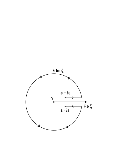
Figure 1: The integration contour in Eq. (7) for the massless case. The physical cut of the strong running coupling $\alpha(-\zeta)$ (see Eq. (9)) is shown along the positive semiaxis of real $\zeta$.

As has been discussed in Section II, for the consistent description of a number of strong interaction processes one has to employ the continuation of the QCD effective charge to the timelike region, in the way given in Eq. (7). For the massless case under consideration it is convenient to choose the integration contour in Eq. (7) in the form presented in Figure 1. Eventually, this leads to the following extension of the invariant charge of Eq. (14) to the timelike domain PRD2

$$\widehat{\alpha}^{(\ell)}_{\text{\scriptsize an}}(s)=\frac{4\pi}{\beta_{0}}\,\int_{w}^{\infty}\!\rho^{(\ell)}(\sigma)\,\frac{d\sigma}{\sigma},\qquad w=\frac{s}{\Lambda^{2}},$$ (20)

where $s=-q^{2}>0$, and the spectral density $\rho^{(\ell)}(\sigma)$ is defined in Eq. (17). The obtained result supports the hypothesis due to Schwinger Schwinger ; Milton concerning the proportionality between the $\beta$ function and the relevant spectral density (see also Ref. MS97 ).

The one-loop effective charge of Eq. (20) has the following asymptotic in the high energy limit $s\to\infty$:

$$\widehat{\alpha}^{(1)}_{\text{\scriptsize an}}(s)\simeq\frac{4\pi}{\beta_{0}}\,\frac{1}{\ln w}\,\left[1-\frac{\pi^{2}}{3}\frac{1}{\ln^{2}\!w}+{\cal O}\!\left(\frac{1}{\ln^{4}\!w},\frac{1}{w}\right)\right].$$ (21)

On the one hand, this running coupling has the correct ultraviolet behavior, determined by the asymptotic freedom. On the other hand, the so-called $\pi^{2}$–terms have also appeared in the expansion (21). As it was noticed in Section II, these terms play a key role in the description of the strong interaction processes in the timelike domain. It is interesting to note that, similarly to the “spacelike” running coupling in the massless case of Eq. (13), the one-loop effective charge (20) also has an enhancement in the infrared domain (see Refs. PRD2 ; Review ):

$$\widehat{\alpha}^{(1)}_{\text{\scriptsize an}}(s)\simeq\frac{4\pi}{\beta_{0}}\,\frac{1}{w\,\ln^{2}\!w},\qquad s\to 0.$$ (22)

However, the type of this singularity differs from that of the invariant charge in Eq. (13) by the logarithmic factor. Nevertheless, it is precisely this feature of the timelike running coupling that enables one to handle the integrals of a specific form over the infrared region, and in particular, to process the experimental data on the inclusive semileptonic branching ratio for the case of the massless pion. In turn, the latter provides one with the relevant estimation of the QCD scale parameter $\Lambda=(508\pm 61)$ MeV, see Section V for the details.

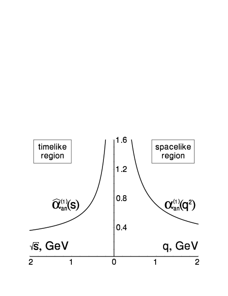
Figure 2: The one-loop massless analytic running coupling in the spacelike (Eq. (16), $q^{2}>0$) and timelike (Eq. (20), $s=-q^{2}>0$) regions. The values of parameters are: $\Lambda=508$ MeV, $n_{\text{\scriptsize f}}=2$ active quarks.

The plots of the functions $\alpha^{(1)}_{\text{\scriptsize an}}(q^{2})$ and $\widehat{\alpha}^{(1)}_{\text{\scriptsize an}}(s)$ are shown in Figure 2. In the ultraviolet limit these expressions have identical behavior determined by the asymptotic freedom. However, there is an asymmetry between them in the intermediate and low energy regions. Thus, the relative difference between these effective charges is about several percent at the scale of the Z boson mass, and increases when approaching the infrared domain. Evidently, this circumstance has to be taken into account when one handles the experimental data (see also review Review and references therein for the details).

It is worthwhile to emphasize that the mass effects have not been included in the formulation of the models for the strong running coupling in the framework of the analytic approach to QCD, so far. Thus, the obtained results can be applied, for example, to the study of the experimental data at high energies, where the masses of the lightest hadrons can be neglected, the pure gluodynamics, and the quenched lattice simulation data (see also Refs. Schrempp ; Review ). However, for the detailed description of the infrared hadron dynamics, the mass effects have to be incorporated into the analytic approach to QCD. The next section is devoted to this task.

IV Massive analytic effective charge

As has been noticed in previous sections, the $\pi$ meson plays a crucial part in the description of the strong interaction processes at low energies. So far the main thrust of the analytic approach to QCD has focused on eliminating intrinsic difficulties of perturbation theory, such as the unphysical singularities of the strong running coupling (see Section III). On the other hand, mass effects within this formalism remain largely unexplored, thus far. Therefore, the objective of this section is to incorporate the effects due to the pion mass into the analytic approach to QCD.

Evidently, the original dispersion relation for the Adler $D$ function Adler (see Eq. (2)) with the nonvanishing mass of the $\pi$ meson is the proper object to study here. Indeed, Eq. (2) implies definite analytic properties in the $q^{2}$ variable for $D(q^{2})$. Namely, the latter has to be an analytic function in the complex $q^{2}$-plane with the only cut beginning at the two–pion threshold $-\infty<q^{2}\leq-4m_{\pi}^{2}$ along the negative semiaxis of real $q^{2}$. However, its approximation in Eq. (6) violates this condition due to the spurious singularities of the perturbative running coupling $\alpha_{\text{\scriptsize s}}(q^{2})$. Nevertheless, this disagreement can be avoided by imposing the analyticity requirement of the form

$$d(q^{2},m_{\pi}^{2})=\int_{4m_{\pi}^{2}}^{\infty}\frac{\varkappa(\sigma)}{\sigma+q^{2}}\,d\sigma$$ (23)

on the right hand-side of Eq. (6). Therefore, the QCD effective charge itself has to satisfy the integral representation

$$\alpha(q^{2},m_{\pi}^{2})=\int_{4m_{\pi}^{2}}^{\infty}\frac{\varrho(\sigma)}{\sigma+q^{2}}\,d\sigma$$ (24)

in this case as well. Otherwise, one would encounter a contradiction between the dispersion relation for the Adler $D$ function of Eq. (2) and its approximation given in Eq. (6). Besides, the condition (24) enforces the validity of relations (7) and (8) for the case of the nonvanishing pion mass.

In general, there are several models for the invariant charge within the analytic approach to QCD (see Section III for the details). This is so by virtue of the fact that the behavior of the strong running coupling $\alpha_{\text{\scriptsize s}}(q^{2})$ at the ultraviolet asymptotic, which is known from perturbation theory, together with the analyticity requirement of the form of Eq. (9) or Eq. (24), is not enough to uniquely determine the relevant spectral density $\varrho(\sigma)$. The model for the analytic invariant charge PRD1 ; PRD2 has proved to be successful in the description of the strong interaction processes of both perturbative and intrinsically nonperturbative nature Review ; QCD03 . We shall therefore adopt the spectral density of Eq. (17) in what follows.

Thus, one arrives at the following integral representation for the massive analytic invariant charge (see also Refs. NPQCD04 ; QCD04 )

$$\alpha^{(\ell)}_{\text{\scriptsize an}}(q^{2},m_{\pi}^{2})=\frac{4\pi}{\beta_{0}}\int_{\chi}^{\infty}\frac{\rho^{(\ell)}(\sigma)}{\sigma+z}\,d\sigma,\qquad z=\frac{q^{2}}{\Lambda^{2}},$$ (25)

where $\rho^{(\ell)}(\sigma)$ denotes the $\ell$-loop spectral density of Eq. (17) and $\chi=4m_{\pi}^{2}/\Lambda^{2}$. It is worth noting from the very beginning that the nonvanishing mass of the $\pi$ meson drastically affects the low energy behavior of this strong running coupling. Indeed, instead of the infrared enhancement in the massless case of Eq. (14), one has here the infrared finite limiting value for the massive invariant charge in Eq. (25),

$$\alpha^{(\ell)}_{\text{\scriptsize 0}}=\frac{4\pi}{\beta_{0}}\int_{\chi}^{\infty}\rho^{(\ell)}(\sigma)\frac{d\sigma}{\sigma},$$ (26)

which depends on the value of the pion mass. At the ultraviolet asymptotic, where the nonperturbative contributions are negligible, the result of Eq. (25) tends to the perturbative running coupling $\alpha^{(\ell)}_{\text{\scriptsize s}}(q^{2})$:

$$\alpha^{(\ell)}_{\text{\scriptsize an}}(q^{2},m_{\pi}^{2})\simeq\alpha^{(\ell)}_{\text{\scriptsize s}}(q^{2})+{\cal O}\!\left[\frac{\Lambda^{2}}{q^{2}},\frac{\Lambda^{2}}{q^{2}}\frac{1}{\ln(q^{2}/\Lambda^{2})},\frac{4m_{\pi}^{2}}{q^{2}}\right].$$ (27)

In this equation the limits $q^{2}\gg\Lambda^{2}$ and $q^{2}\gg 4m_{\pi}^{2}$ are assumed. In particular, the one-loop effective charge of Eq. (25) reads for $q^{2}\gg 4m_{\pi}^{2}$

$$\alpha^{(1)}_{\text{\scriptsize an}}(q^{2},m_{\pi}^{2}) \simeq \alpha^{(1)}_{\text{\scriptsize s}}(q^{2})-\frac{4\pi}{\beta_{0}}\frac{1}{z\ln z}$$ (28)

$$-\frac{4}{\beta_{0}}\frac{1}{z}\left[\frac{\pi}{2}+(\chi+1)\arctan\left(\frac{\ln\chi}{\pi}\right)\right]$$

$$+\frac{4}{\beta_{0}}\frac{1}{z}\int_{-\infty}^{\ln\chi}e^{y}\arctan\left(\frac{y}{\pi}\right)\,dy.$$

It is worthwhile to mention also that in the limit of massless pion $m_{\pi}=0$ the effective charge (25) coincides with the running coupling of Eq. (14).

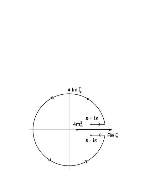
Figure 3: The integration contour in Eq. (7) for the case of the massive pion. The physical cut of the effective charge $\alpha(-\zeta,m_{\pi}^{2})$ (see Eq. (24)) is shown along the positive semiaxis of real $\zeta$.

In order to handle the strong interaction processes involving the timelike kinematic variable one first has to relate the experimental data with the perturbative results (see Section II). For practical purposes it is convenient to employ here the extension of the spacelike running coupling to the timelike domain given by Eq. (7). The analytic properties in the $q^{2}$ variable of the QCD invariant charge $\alpha(q^{2})$ are different for the massless (9) and massive (24) cases (see Figures 1 and 3, respectively). Thus, the continuation (7) of the massive strong running coupling (25) to the timelike region results in (see Refs. NPQCD04 ; QCD04 also)

$$\widehat{\alpha}^{(\ell)}_{\text{\scriptsize an}}(s,m_{\pi}^{2})=\frac{4\pi}{\beta_{0}}\int_{w}^{\infty}\theta(\sigma-\chi)\,\rho^{(\ell)}(\sigma)\frac{d\sigma}{\sigma},\qquad w=\frac{s}{\Lambda^{2}},$$ (29)

where $s=-q^{2}\geq 0$, $\,\theta(x)$ stands for the Heaviside step-function (see, e.g., Ref. AS ), $\rho^{(\ell)}(\sigma)$ is the $\ell$-loop spectral density defined in Eq. (17), and $\chi=4m_{\pi}^{2}/\Lambda^{2}$.

Let us address now the basic features of the running coupling in Eq. (29). First of all, it is very interesting to note here that the effective charges of Eq. (25) and Eq. (29) have a common finite value in the infrared limit $|q^{2}|\to 0$, given by Eq. (26). Second, the timelike massive effective coupling of Eq. (29) has the “plateau–like” behavior in the deep infrared domain:

$$\widehat{\alpha}^{(\ell)}_{\text{\scriptsize an}}(s,m_{\pi}^{2})=\alpha^{(\ell)}_{\text{\scriptsize 0}},\qquad 0\leq\sqrt{s}\leq 2m_{\pi}.$$ (30)

Besides, for $\sqrt{s}>2m_{\pi}$ there is no difference between the massless and massive timelike running couplings of Eq. (20) and Eq. (29), respectively, since the mass of the $\pi$ meson affects the timelike effective charge (29) only in the region $\sqrt{s}\leq 2m_{\pi}$, where it does not run (see Figure 4). Therefore, in the ultraviolet asymptotic $s\to\infty$, the expansion (21), which accounts for the $\pi^{2}$-terms, also holds for the running coupling of Eq. (29). The hypothesis due to Schwinger Schwinger ; Milton concerning the proportionality between the $\beta$ function and the relevant spectral density holds for the massive timelike effective charge of Eq. (29) as well. Apparently, in the limit of vanishing pion mass $m_{\pi}\to 0$ the results of this section reproduce the massless case described in Section III.

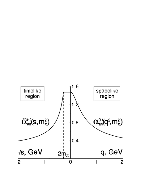
Figure 4: The one–loop massive analytic effective charge in the spacelike and timelike domains (Eqs. (25) and (29), respectively). The values of parameters are: $\Lambda=623$ MeV, $n_{\text{\scriptsize f}}=2$ active quarks.

It is worth noting here that some other models for the QCD effective charge also display a plateau similar to (30) in the infrared domain. In particular, the aforementioned optimized perturbation theory method OPTEpEm predicts the stagnation of the timelike effective coupling in the region $\sqrt{s}\lesssim 300$ MeV, in striking coincidence with the result obtained in Eq. (30). Moreover, the so-called “H–model”, with a similar freezing of the effective charge to a constant value in the infrared domain, has proved to be useful in studying of the dynamical chiral symmetry breaking (see, e.g., Ref. Hig84 ).

V Inclusive $\tau$ lepton decay

In order to draw a quantitative conclusion on the low energy behavior of a model for the strong running coupling, one needs the relevant estimation of the QCD scale parameter $\Lambda$. The latter can be extracted, for example, from the experimental data on the strong interaction processes. Among them, the measurement of the $\tau$ decay width is most suitable for our purposes, since these data are fairly precise, and this process probes the infrared hadron dynamics at energies below the $\tau$ lepton mass $0\leq\sqrt{s}\leq M_{\tau}$. Let us turn now to the study of this hadron process, restricting ourselves to the one–loop level at this stage.

The experimentally measurable quantity here is the inclusive semileptonic branching ratio

$$R_{\tau}=\frac{\Gamma(\tau^{-}\to\text{hadrons}^{-}\,\nu_{\tau})}{\Gamma(\tau^{-}\to e^{-}\,\bar{\nu}_{e}\,\nu_{\tau})}.$$ (31)

One can split this ratio into three parts, namely $R_{\tau}=R_{\tau,\text{\tiny V}}+R_{\tau,\text{\tiny A}}+R_{\tau,\text{\tiny S}}$. The terms $R_{\tau,\text{\tiny V}}$ and $R_{\tau,\text{\tiny A}}$ account for the contributions to Eq. (31) of the decay modes with the light quarks only, and they correspond to the vector (V) and axial–vector (A) quark currents, respectively. The accuracy of the experimental measurement of these terms is several times higher than that of the strange width ratio $R_{\tau,\text{\tiny S}}$, which accounts for the contribution to Eq. (31) of the decay modes with the $s$ quark. Thus, let us proceed with the nonstrange part of the ratio $R_{\tau}$ (31) associated with the vector quark currents

$$R_{\tau,\text{\tiny V}}=\frac{N_{\text{\scriptsize c}}}{2}\,|V_{\text{\scriptsize ud}}|^{2}\,S_{\text{\tiny EW}}\left(1+\delta^{\prime}_{\text{\tiny EW}}+\delta_{\text{\tiny QCD}}\right),$$ (32)

see Refs. BDP ; BNP ; APTTau for detailed discussion of this issue. In Eq. (32) $N_{\text{\scriptsize c}}=3$ is the number of colors, $|V_{\text{\scriptsize ud}}|=0.9738\pm 0.0005$ denotes the Cabibbo–Kobayashi–Maskawa matrix element PDG04 , $S_{\text{\tiny EW}}=1.0194\pm 0.0050$ and $\delta^{\prime}_{\text{\tiny EW}}=0.0010$ are the electroweak corrections BNP ; EWF , and $\delta_{\text{\tiny QCD}}$ stands for the strong correction. The recent measurements of the ratio (32) gave $R_{\tau,\text{\tiny V}}=1.775\pm 0.017$ (ALEPH Collaboration, Ref. ALEPH ) and $R_{\tau,\text{\tiny V}}=1.764\pm 0.016$ (OPAL Collaboration, Ref. OPAL ). Assuming that these data have equal statistical weights, one arrives at the averaged value

$$R_{\tau,\text{\tiny V}}=1.769\pm 0.017.$$ (33)

In the framework of the approach in hand the strong correction in Eq. (32) at the one-loop level takes the form

$$\delta^{(1)}_{\text{\tiny QCD}}=\frac{2}{\pi}\int_{0}^{M_{\tau}^{2}}\left(1-\frac{s}{M_{\tau}^{2}}\right)^{\!2}\left(1+2\frac{s}{M_{\tau}^{2}}\right)\widehat{\alpha}^{(1)}_{\text{\scriptsize}}(s)\frac{ds}{M_{\tau}^{2}},$$ (34)

see, e.g, papers APTTau ; PRD2 ; Review and references therein. In Eq. (34) $\widehat{\alpha}^{(1)}_{\text{\scriptsize}}(s)$ is the one-loop strong running coupling in the timelike region, and $M_{\tau}=(1776.99_{-0.26}^{+0.29})$ MeV denotes the mass of the $\tau$ lepton PDG04 . As was shown in previous sections, the mass of the $\pi$ meson entering the dispersion relation for the Adler $D$ function (2) affects the low energy behavior of the QCD effective charge $\widehat{\alpha}_{\text{\scriptsize}}(s)$. Consequently, handling the experimental data on the inclusive $\tau$ lepton decay is different for the cases of massless and massive pion. In order to demonstrate how the estimation of the QCD scale parameter $\Lambda$ is affected by the nonvanishing mass of the $\pi$ meson, let us study both instances.

For the limit of massless pion $m_{\pi}=0$, the one-loop strong correction $\delta_{\text{\tiny QCD}}$ to the $R_{\tau,\text{\tiny V}}$ ratio (32) is given by Eq. (34), with $\widehat{\alpha}^{(1)}_{\text{\scriptsize}}(s)$ being the one-loop massless effective charge of Eq. (20). Although the latter possesses the enhancement at $s\to 0$ (see Eq. (22)), the resulting singularity is integrable. Then, it is useful to represent the QCD correction in a more convenient form

$$\delta^{(1)}_{\text{\tiny QCD}}(M_{\tau}^{2}) = \frac{4}{\beta_{0}}\int_{0}^{1}\left(\xi^{3}-2\xi^{2}+2\right)\rho^{(1)}(\xi\mu)\,d\xi$$ (35)

$$+\frac{1}{\pi}\widehat{\alpha}^{(1)}_{\text{\scriptsize an}}(M_{\tau}^{2}),$$

where $\widehat{\alpha}^{(1)}_{\text{\scriptsize an}}(s)$ is the running coupling (20), $\rho^{(1)}(\sigma)$ denotes the one-loop spectral density (19), and the notations $\xi=s/M_{\tau}^{2}$ and $\mu=M_{\tau}^{2}/\Lambda^{2}$ are used. For the experimental data given in Eq. (33) one gets the value $\Lambda=(508\pm 61)$ MeV for the QCD scale parameter. This estimation corresponds to $n_{\text{\scriptsize f}}=2$ active quarks, and its uncertainty is due to the errors in the values of $R_{\tau,\text{\tiny V}}$, $|V_{\text{\scriptsize ud}}|$, $S_{\text{\tiny EW}}$, and $M_{\tau}$. The relevant behavior of the massless analytic invariant charge in the spacelike and timelike regions (Eqs. (16) and (20), respectively) is shown in Figure 2.

Let us proceed now to the case of the nonvanishing pion mass. Here, the one-loop QCD correction to the $R_{\tau,\text{\tiny V}}$ ratio reads as

$$\delta^{(1)}_{\text{\tiny QCD}}(M_{\tau}^{2},m_{\pi}^{2}) = \frac{2}{\pi}\int_{0}^{M_{\tau}^{2}}\left(1-\frac{s}{M_{\tau}^{2}}\right)^{\!2}$$ (36)

$$\times\!\left(\!1+2\frac{s}{M_{\tau}^{2}}\!\right)\!\widehat{\alpha}^{(1)}_{\text{\scriptsize an}}(s,m_{\pi}^{2})\frac{ds}{M_{\tau}^{2}},$$

where $\widehat{\alpha}^{(1)}_{\text{\scriptsize an}}(s,m_{\pi}^{2})$ is the one-loop massive analytic charge of Eq. (29) and $m_{\pi}=(134.9766\pm 0.0006)$ MeV stands for the $\pi^{0}$ meson mass PDG04 . In general, in the framework of the analytic approach there is no need to involve the contour integration in Eq. (34), since the effective charge $\widehat{\alpha}_{\text{\scriptsize}}(s)$, appearing in the integrand, contains no unphysical singularities in the region $s\geq 0$. In other words, the integration in Eq. (34) can be performed in a straightforward way. Thus, one can cast the strong correction (36) into a convenient form

$$\delta^{(1)}_{\text{\tiny QCD}}(M_{\tau}^{2},m_{\pi}^{2}) = \frac{4}{\beta_{0}}\int_{\xi_{0}}^{1}\left(\xi^{3}-2\xi^{2}+2\right)\rho^{(1)}(\xi\mu)\,d\xi$$ (37)

$$+\frac{1}{\pi}\widehat{\alpha}^{(1)}_{\text{\scriptsize an}}(M_{\tau}^{2},m_{\pi}^{2}),$$

where $\xi_{0}=4m_{\pi}^{2}/M_{\tau}^{2}$ and the other notations have been explained above. For the experimental data (33) the estimation $\Lambda=(623\pm 81)$ MeV has been obtained for $n_{\text{\scriptsize f}}=2$ active quarks. The uncertainty here is because of the errors of $R_{\tau,\text{\tiny V}}$, $|V_{\text{\scriptsize ud}}|$, $S_{\text{\tiny EW}}$, $M_{\tau}$, and $m_{\pi}$. The corresponding infrared limiting value of the massive effective charge (26) is $\alpha^{(1)}_{\text{\scriptsize 0}}=1.475\pm 0.170$. The low energy behavior of the analytic running coupling in the spacelike and timelike domains (Eqs. (25) and (29), respectively) is presented in Figure 4.

Thus, in the framework of the approach in hand it proves to be important to take into account the mass of the $\pi$ meson in processing the low energy QCD data. Specifically, the relative difference between the obtained estimations of the scale parameter $\Lambda$ for the massive and massless cases is about $20\,\%$. This is so by virtue of the fact that the contribution to the strong correction (34) of the effects due to the pion mass

$$\Delta\delta^{(1)}_{\text{\tiny QCD}}(M_{\tau}^{2},m_{\pi}^{2})=\frac{4}{\beta_{0}}\int_{0}^{\xi_{0}}\left(\xi^{3}-2\xi^{2}+2\right)\rho^{(1)}(\xi\mu)\,d\xi$$ (38)

turns out to be significant. At the same time, since the scales involved in the integral (38) are very low, for some models for the analytic running coupling the difference between the limits of massive and massless $\pi$ meson may not be so sizable. For example, in the case of the Shirkov–Solovtsov model ShSol , where the relevant spectral density reads as $\rho^{(1)}_{\text{\scriptsize ss}}(\sigma)=1/(\ln^{2}\!\sigma+\pi^{2})$, the relative difference between the values of the QCD scale parameter, extracted from the experimental data on the inclusive $\tau$ lepton decay (33), is about $1\,\%$, but the obtained estimations appear to be rather large. Namely, at the one-loop level with $n_{\text{\scriptsize f}}=2$ active quarks one gets the values $\Lambda=(965^{+280}_{-212})$ MeV for the case of the massless $\pi$ meson, and $\Lambda=(976^{+281}_{-213})$ MeV for the nonvanishing pion mass.

VI Applicability to the chiral symmetry breaking

Based on the study of gauge invariant Schwinger–Dyson equations, Cornwall proposed a long time ago that the self-interactions of gluons give rise to a dynamical gluon mass, while preserving at the same time the local gauge symmetry of the theory Cornwall:1982zr . This gluon “mass” is not a directly measurable quantity, but has to be related with other physical quantities, such as the glueball spectrum, the energy needed to pop two gluons out of the vacuum, the QCD string tension, or the QCD vacuum energy (see paper Aguilar:2002tc and references therein).

One of the main phenomenological implications of this analysis is that the presence of the gluon mass $m_{g}$ saturates the running of the strong coupling at low energies. Namely, instead of increasing indefinitely in the infrared, as perturbation theory predicts, it “freezes” at a finite value, determined by the gluon mass. In particular, the nonperturbative effective coupling obtained in Ref. Cornwall:1982zr is given by

$$\alpha_{\text{\tiny C}}(q^{2})=\frac{4\pi}{\beta_{0}}\frac{1}{\ln\!\left[z+4M_{g}^{2}(q^{2})/\Lambda^{2}\right]},\qquad z=\frac{q^{2}}{\Lambda^{2}},$$ (39)

where $M_{g}(q^{2})$ denotes the dynamical gluon mass

$$M^{2}_{g}(q^{2})=m_{g}^{2}\left[\frac{\ln\!\left(z+4m_{g}^{2}/\Lambda^{2}\right)}{\ln\!\left(4m_{g}^{2}/\Lambda^{2}\right)}\right]^{-\frac{12}{11}}.$$ (40)

Here the nontrivial dependence of the dynamically generated gluon mass (40) on the momentum $q^{2}$ is crucial for the renormalizability of the theory. The running coupling (39) has the infrared finite limiting value $\alpha_{\text{\tiny C}}(0)=4\pi\left[\beta_{0}\ln(4m_{g}^{2}/\Lambda^{2})\right]^{-1}$. It is worth noting that the above equation makes sense only for the gluon mass satisfying $m_{g}>\Lambda/2$. For a typical values of $m_{g}=500$ MeV and $\Lambda=300$ MeV, one obtains for the case of the pure gluodynamics ($n_{\text{\scriptsize f}}=0$) an estimation $\alpha_{\text{\tiny C}}(0)\simeq 0.5$. An independent analysis presented in Ref. Cornwall:1989gv yields a maximum allowed value for $\alpha_{\text{\tiny C}}(0)$ of about 0.6. The incorporation of fermions into the effective charge Papavassiliou:1991hx does not change the picture qualitatively (at least for the quark masses of the order of $\Lambda$), resulting in an approximate expression

$$\alpha_{\text{\scriptsize cp}}(q^{2})=\frac{4\pi}{11\ln(z+\chi_{g})-2n_{\text{\scriptsize f}}\ln(z+\chi_{q})/3}.$$ (41)

In this equation $\chi_{g}=4m_{g}^{2}/\Lambda^{2}$, $\chi_{q}=4m_{q}^{2}/\Lambda^{2}$, a light quark constituent mass is $m_{q}=350$ MeV PDG04 , and $m_{g}=(500\pm 100)$ MeV stands for the gluon mass. The effective coupling of Eq. (39) was the focal point of extensive scrutiny, and has been demonstrated to furnish an unified description of a wide variety of the low energy QCD data Cristina .

Figure 5: Graphical representation of the gap equation (42).

In general, an important unresolved question in this context is the incorporation of the QCD effective charge into the standard Schwinger–Dyson equation governing the dynamics of the quark propagator $S(p)$

$$S^{-1}(p)=S_{0}^{-1}(p)-g^{2}\int\frac{d^{4}k}{(2\pi)^{4}}\gamma_{\mu}\,S\,\Gamma_{\nu}\,\Delta^{\mu\nu},$$ (42)

see Figure 5 also. In particular, since QCD is not a fixed point theory, the usual QED–inspired gap equation must be modified, in order to incorporate the running charge and asymptotic freedom. The usual way of accomplishing this eventually reduces to the replacement $1/k^{2}\to\alpha(k^{2})/k^{2}$ in the corresponding kernel of the gap equation, where $\alpha(k^{2})$ is the QCD running coupling. The inclusion of $\alpha(k^{2})$ is essential for arriving at an integral equation for $S(p)$ which is well-behaved in the ultraviolet. Indeed, the additional logarithm in the denominator of the kernel due to the running coupling $\alpha(k^{2})$ improves the convergence of the integral. However, since the perturbative form of $\alpha(k^{2})$ diverges at low energies as $1/\ln(k^{2}/\Lambda^{2})$ when $k^{2}\to\Lambda^{2}$, some form of the infrared regularization for the invariant charge $\alpha(k^{2})$ is needed, whose details depend on the specific assumptions one is making regarding the nonperturbative hadron dynamics. At this point the issue of the critical coupling makes its appearance. Specifically, as is well-known, there is a critical infrared limiting value of the running coupling, to be denoted by $\alpha_{\text{\scriptsize cr}}$, below which there are no nontrivial solutions to the resulting gap equation, i.e., there is no chiral symmetry breaking, see Figure 6. Thus, the invariant charge $\alpha(k^{2})$ employed within the gap equation must be such that (i) it gives rise to a nonsingular answer, (ii) it reaches large enough values at $k^{2}\to 0$ in order to overcome $\alpha_{\text{\scriptsize cr}}$, and (iii) it does not contradict existing low-energy experimental results.

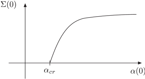
Figure 6: A typical dependence of $\Sigma(0)$ on the infrared limiting value of the QCD effective charge $\alpha(0)$, $\,S^{-1}(p)=A(p)p/+\Sigma(p)$.

The incorporation of the effective charge of Eq. (39) into a gap equation has been studied for the first time in Ref. Haeri:1990yj . There it was concluded that chiral symmetry breaking solutions for $\Sigma(p)$ could be obtained only for unnaturally small values of the gluon mass, namely $m_{g}/\Lambda\simeq 0.8$. This is so because the typical value of $\alpha_{\text{\scriptsize cr}}$ found in the standard treatment of the gap equation is $\alpha_{\text{\scriptsize cr}}\simeq 1.2$ (see, e.g., Ref. Atkinson ), which is what the expression for $\alpha_{\text{\tiny C}}(0)$ yields for the above ratio of $m_{g}/\Lambda$. This issue was further investigated in Ref. Papavassiliou:1991hx , where a system of coupled gap and vertex equations was considered. The upshot of this study was that no consistent solutions to the system of integral equations could be found, due to the fact that the allowed values for $\alpha(0)$, dictated by the vertex equation, were significantly lower than $\alpha_{\text{\scriptsize cr}}$, i.e., not large enough to trigger chiral symmetry breaking. A similar analysis was presented in Ref. Aguilar:2001zy , together with several other models for the nonperturbative QCD running coupling Aguilar:2000kp .

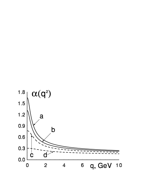
Figure 7: Comparison of the massive analytic running coupling (25) (solid curves) with the effective charge (41) (dashed curves). The values of parameters are: $n_{\text{\scriptsize f}}=2$ active quarks, $\Lambda=704$ MeV (a), $\Lambda=542$ MeV (b), gluon mass $m_{g}=400$ MeV and $\Lambda=350$ MeV (c), gluon mass $m_{g}=600$ MeV and $\Lambda=150$ MeV (d).

In what follows we will suggest a possible resolution of this problem, inspired by the infrared behavior of the massive analytic invariant charge of Eq. (25). The basic observation is captured in Figure 7. Namely, the effective charge with a gluon mass (dashed curves) and the analytic charge (solid curves) coincide for a large range of momenta, and they only begin to differ appreciably in the deep infrared domain $k^{2}\lesssim\Lambda^{2}$. In this region the analytic charge (25) rises abruptly, almost doubling its size between $k^{2}=\Lambda^{2}$ and $k^{2}=0$, whereas the running coupling (41) in the same momentum interval remains essentially fixed to a value of about 0.6. A possible picture that emerges from this observation is the following. It may be that the concept of the dynamically generated gluon mass fails to capture all the relevant dynamics in the very deep infrared, where confinement or other nonperturbative effects make their appearance. At that point it could be preferable to switch to a description in terms of the analytic charge (25), which (i) coincides with that of Cornwall in the region where the latter furnishes a successful description of data, and (ii) since it overcomes the critical value $\alpha_{\text{\scriptsize cr}}$, offers the possibility of accounting for chiral symmetry breaking at the level of gap equations.

VII Conclusions

In this paper the effects due to the mass of the $\pi$ meson are incorporated into the analytic approach to QCD. The nonvanishing pion mass gives rise to an infrared finite limiting value for the QCD effective charge. Besides, the latter acquires the plateau-like behavior in the deep infrared domain of the timelike region $0\leq\sqrt{s}\leq 2m_{\pi}$. It is of a particular interest to note that such stagnation is also predicted by a number of phenomenological models for the strong running coupling. The developed analytic effective charge is applied to processing the experimental data on the inclusive $\tau$ lepton decay. The effects due to the pion mass play a substantial role here, affecting the estimation of the QCD scale parameter $\Lambda$. A quantitative conclusion on the applicability of the obtained massive running coupling to the study of chiral symmetry breaking is drawn.

It would be interesting to further scrutinize the developed approach. First of all, it is of particular relevance to include the higher order perturbative corrections in the study of the experimental data on the inclusive $\tau$ lepton decay. Moreover, it might also be important to incorporate the nonperturbative terms, arising from the operator product expansion (see also Ref. Maxwell ) and from the so-called nonlocal chiral quark model Dorokhov , into the Adler $D$ function. In addition, a detailed study of the gap equation, with the analytic charged plugged into it, is needed in order to verify if indeed one encounters nontrivial solutions, whose size is phenomenologically relevant. Specifically, one should check by making use of, e.g., the Pagels–Stokar method Pagels:1979hd , whether the solutions obtained for $\Sigma(p)$ can reproduce a reasonable value of the pion-decay constant $f_{\pi}$. It is also interesting to apply the developed model to the study of the pion electromagnetic form factor $F_{\pi}(q)$ (see paper Stefanis and references therein). At the same time, a crucial point to explore is whether the massive analytic effective charge satisfies a variety of phenomenological constraints, imposed by the low energy experimental data on the infrared behavior of the QCD running coupling, see, e.g., papers Doksh ; Cristina and references therein.

- (1) D.J. Gross and F. Wilczek, Phys. Rev. Lett. 30, 1343 (1973); H.D. Politzer, ibid. 30, 1346 (1973); G. ’t Hooft, report at the Conference on Yang–Mills Fields (Marseille, France, 1972).
- (2) E.C.G. Stuckelberg and A. Petermann, Helv. Phys. Acta 24, 317 (1951); 26, 499 (1953); M. Gell–Mann and F.E. Low, Phys. Rev. 95, 1300 (1954); N.N. Bogoliubov and D.V. Shirkov, Dokl. Akad. Nauk SSSR 103, 203 (1955); 103, 391 (1955); Nuovo Cimento 3, 845 (1956).
- (3) N.N. Bogoliubov and D.V. Shirkov, Introduction to the Theory of Quantized Fields (Interscience, New York, 1980).
- (4) W. Fischler, Nucl. Phys. B 129, 157 (1977); T. Appelquist, M. Dine, and I.J. Muzinich, Phys. Lett. B 69, 231 (1977); Phys. Rev. D 17, 2074 (1978); M. Peter, Phys. Rev. Lett. 78, 602 (1997); Nucl. Phys. B 501, 471 (1997).
- (5) G.S. Bali et al. (SESAM and TL Collaborations), Phys. Rev. D 62, 054503 (2000); G.S. Bali, Phys. Rep. 343, 1 (2001); C. Bernard et al., Phys. Rev. D 62, 034503 (2000); S. Necco and R. Sommer, Nucl. Phys. B 622, 328 (2002); T.T. Takahashi, H. Suganuma, Y. Nemoto, and H. Matsufuru, Phys. Rev. D 65, 114509 (2002); S. Aoki et al. (JLQCD Collaboration), ibid. 68, 054502 (2003).
- (6) B.M. Barbashov and V.V. Nesterenko, Introduction to the Relativistic String Theory (World Scientific, Singapore, 1990).
- (7) W. Celmaster and F.S. Henyey, Phys. Rev. D 18, 1688 (1978); D.B. Lichtenberg and J.G. Wills, Nuovo Cimento A 47, 483 (1978); R. Levine and Y. Tomozawa, Phys. Rev. D 19, 1572 (1979); J.L. Richardson, Phys. Lett. B 82, 272 (1979); W. Buchmuller, G. Grunberg, and S.-H.H. Tye, Phys. Rev. Lett. 45, 103 (1980).
- (8) W. Lucha, F.F. Schoberl, and D. Gromes, Phys. Rept. 200, 127 (1991); N. Brambilla and A. Vairo, arXiv:hep-ph/9904330; V.V. Kiselev, A.E. Kovalsky, and A.I. Onishchenko, Phys. Rev. D 64, 054009 (2001).
- (9) A. Ringwald and F. Schrempp, Phys. Lett. B 459, 249 (1999).
- (10) D.A. Smith and M.J. Teper (UKQCD Collaboration), Phys. Rev. D 58, 014505 (1998).
- (11) A.V. Nesterenko, Phys. Rev. D 62, 094028 (2000).
- (12) A.V. Nesterenko, Phys. Rev. D 64, 116009 (2001).
- (13) F. Schrempp, J. Phys. G 28, 915 (2002).
- (14) A.V. Nesterenko, Int. J. Mod. Phys. A 18, 5475 (2003).
- (15) P.M. Stevenson, Phys. Rev. D 23, 2916 (1981).
- (16) A.C. Mattingly and P.M. Stevenson, Phys. Rev. D 49, 437 (1994).
- (17) G. Grunberg, Phys. Rev. D 29, 2315 (1984).
- (18) S.J. Brodsky, G.P. Lepage, and P.B. Mackenzie, Phys. Rev. D 28, 228 (1983).
- (19) S. Ciulli and J. Fischer, Nucl. Phys. 24, 465 (1961); J. Fischer, Fortschr. Phys. 42, 665 (1994); I. Caprini and J. Fischer, Phys. Rev. D 60, 054014 (1999); 62, 054007 (2000); 68, 114010 (2003).
- (20) V. Elias, D.G.C. McKeon, and T.G. Steele, Phys. Rev. D 69, 045015 (2004); Int. J. Mod. Phys. A 18, 3417 (2003); V. Elias, arXiv:hep-ph/0305187.
- (21) M.R. Ahmady et al., Nucl. Phys. B 655, 221 (2003); Phys. Rev. D 66, 014010 (2002); 67, 034017 (2003).
- (22) P.J. Redmond, Phys. Rev. 112, 1404 (1958); P.J. Redmond and J.L. Uretsky, Phys. Rev. Lett. 1, 147 (1958); N.N. Bogoliubov, A.A. Logunov, and D.V. Shirkov, Zh. Eksp. Teor. Fiz. 37, 805 (1959) [Sov. Phys. JETP 37, 574 (1960)].
- (23) J.D. Bjorken, report SLAC-PUB-5103 (1989).
- (24) Y.L. Dokshitzer, G. Marchesini, and B.R. Webber, Nucl. Phys. B 469, 93 (1996).
- (25) D.V. Shirkov and I.L. Solovtsov, JINR Rapid Comm. 2, 5 (1996); Phys. Rev. Lett. 79, 1209 (1997).
- (26) D.V. Shirkov, Teor. Mat. Fiz. 119, 55 (1999) [Theor. Math. Phys. 119, 438 (1999)]; I.L. Solovtsov and D.V. Shirkov, Teor. Mat. Fiz. 120, 482 (1999) [Theor. Math. Phys. 120, 1220 (1999)].
- (27) A.V. Nesterenko, Nucl. Phys. B (Proc. Suppl.) 133, 59 (2004).
- (28) K.A. Milton and I.L. Solovtsov, Phys. Rev. D 55, 5295 (1997); 59, 107701 (1999).
- (29) J.M. Cornwall, Phys. Rev. D 26, 1453 (1982).
- (30) A. Peterman, Phys. Rep. 53, 157 (1979); A.J. Buras, Rev. Mod. Phys. 52, 199 (1980).
- (31) M.R. Pennington and G.G. Ross, Phys. Lett. B 102, 167 (1981).
- (32) S.L. Adler, Phys. Rev. D 10, 3714 (1974).
- (33) A.V. Radyushkin, Joint Institute for Nuclear Research report No. 2–82–159 (1982); JINR Rapid Comm. 4, 9 (1996); arXiv:hep-ph/9907228.
- (34) N.V. Krasnikov and A.A. Pivovarov, Phys. Lett. B 116, 168 (1982).
- (35) T. Appelquist and H. Georgi, Phys. Rev. D 8, 4000 (1973); A. Zee, ibid. D 8, 4038 (1973).
- (36) S.G. Gorishny, A.L. Kataev, and S.A. Larin, Phys. Lett. B 259, 144 (1991).
- (37) L.R. Surguladze and M.A. Samuel, Phys. Rev. Lett. 66, 560 (1991); textbf66, 2416(E) (1991).
- (38) D.V. Shirkov, Eur. Phys. J. C 22, 331 (2001); Teor. Mat. Fiz. 127, 3 (2001) [Theor. Math. Phys. 127, 409 (2001)].
- (39) K.A. Milton, I.L. Solovtsov, and O.P. Solovtsova, Phys. Rev. D 64, 016005 (2001); D 65, 076009 (2002); K.A. Milton, I.L. Solovtsov, O.P. Solovtsova, and V.I. Yasnov, Eur. Phys. J. C 14, 495 (2000).
- (40) R. Jost and H. Lehmann, Nuovo Cimento 5, 1598 (1957); F.J. Dyson, Phys. Rev. 110, 1460 (1958); N.N. Bogoliubov, V.S. Vladimirov, and A.N. Tavkhelidze, Theor. Math. Phys. 12, 305 (1972).
- (41) A.V. Nesterenko and I.L. Solovtsov, Mod. Phys. Lett. A 16, 2517 (2001).
- (42) D.V. Shirkov, Teor. Mat. Fiz. 132, 484 (2002) [Theor. Math. Phys. 132, 1309 (2002)].
- (43) D.V. Shirkov, in Proceedings of the Eleventh International QCD Conference (5–10 July 2004, Montpellier, France) (to be published); arXiv:hep-ph/0408272.
- (44) A.V. Nesterenko, Int. J. Mod. Phys. A 19, 3471 (2004).
- (45) A.V. Nesterenko, Mod. Phys. Lett. A 15, 2401 (2000).
- (46) J. Schwinger, Proc. Natl. Acad. Sci. USA 71, 3024 (1974); 71, 5047 (1974).
- (47) K.A. Milton, Phys. Rev. D 10, 4247 (1974).
- (48) A.V. Nesterenko and J. Papavassiliou, in Proceedings of the Eighth Workshop on Nonperturbative QCD (7–11 June 2004, Paris, France) (to be published); arXiv:hep-ph/0409220.
- (49) A.V. Nesterenko and J. Papavassiliou, in Proceedings of the Eleventh International QCD Conference (5–10 July 2004, Montpellier, France) (to be published); arXiv:hep-ph/0410072.
- (50) M. Abramowitz and I.A. Stegun (Eds.), Handbook of Mathematical Functions (Dover, New York, 1972).
- (51) K. Higashijima, Phys. Rev. D 29, 1228 (1984).
- (52) E. Braaten, Phys. Rev. Lett. 60, 1606 (1988); Phys. Rev. D 39, 1458 (1989); F. Le Diberder and A. Pich, Phys. Lett. B 286, 147 (1992).
- (53) E. Braaten, S. Narison, and A. Pich, Nucl. Phys. B 373, 581 (1992).
- (54) S. Eidelman et al. (Particle Data Group), Phys. Lett. B 592, 1 (2004).
- (55) W.J. Marciano and A. Sirlin, Phys. Rev. Lett. 61, 1815 (1988); 56, 22 (1986); E. Braaten and C.S. Li, Phys. Rev. D 42, 3888 (1990).
- (56) R. Barate et al. (ALEPH Collaboration), Eur. Phys. J. C 4, 409 (1998).
- (57) K. Ackerstaff et al. (OPAL Collaboration), Eur. Phys. J. C 7, 571 (1999).
- (58) A.C. Aguilar, A.A. Natale, and P.S. Rodrigues da Silva, Phys. Rev. Lett. 90, 152001 (2003).
- (59) D.V. Shirkov, Phys. Atom. Nucl. 62, 1928 (1999).
- (60) J.M. Cornwall and J. Papavassiliou, Phys. Rev. D 40, 3474 (1989).
- (61) J. Papavassiliou and J.M. Cornwall, Phys. Rev. D 44, 1285 (1991).
- (62) A.C. Aguilar, A. Mihara, and A.A. Natale, Int. J. Mod. Phys. A 19, 249 (2004).
- (63) B. Haeri and M.B. Haeri, Phys. Rev. D 43, 3732 (1991).
- (64) D. Atkinson, P.W. Johnson, and K. Stam, Phys. Rev. D 37, 2996 (1988).
- (65) A.C. Aguilar, A. Mihara, and A.A. Natale, Phys. Rev. D 65, 054011 (2002).
- (66) A.C. Aguilar, A.A. Natale, and R. Rosenfeld, Phys. Rev. D 62, 094014 (2000).
- (67) D.M. Howe and C.J. Maxwell, Phys. Rev. D 70, 014002 (2004).
- (68) A.E. Dorokhov and W. Broniowski, Eur. Phys. J. C 32, 79 (2003); I.V. Anikin, A.E. Dorokhov, and L. Tomio, Phys. Part. Nucl. 31, 509 (2000) [Fiz. Elem. Chast. Atom. Yadra 31, 1023 (2000)]; A.E. Dorokhov, arXiv:hep-ph/0405153.
- (69) H. Pagels and S. Stokar, Phys. Rev. D 20, 2947 (1979).
- (70) A.P. Bakulev, K. Passek-Kumericki, W. Schroers, and N.G. Stefanis, Phys. Rev. D 70, 033014 (2004); N.G. Stefanis, arXiv:hep-ph/0410245.
- (71) Yu.L. Dokshitzer and B.R. Webber, Phys. Lett. B 352, 451 (1995); Yu.L. Dokshitzer, V.A. Khoze, and S.I. Troyan, Phys. Rev. D 53, 89 (1996).