Effective Lagrangian for Charged Higgs Couplings

Abstract

The effective Lagrangian including one loop corrections is deduced for the couplings of the charged Higgs with quarks and leptons, and with charginos and neutralinos. The effect of the one loop corrections is found to be quite significant in a number of sectors. The effective Lagrangian is then used to analyze the decay of the charged Higgs into a number of decay channels. Specifically we consider the decay of $H^{+}(H^{-})$ into the decay modes $t\bar{b}$ ($\bar{t}b$), $\bar{\tau}\nu_{\tau}$ ($\tau\bar{\nu}_{\tau}$), and $\chi_{i}^{+}\chi_{j}^{0}(\chi_{i}^{-}\chi_{j}^{0})$ (i=1,2; j=1-4). The loop corrections to these decay modes are also found to be quite significant lying in the range 20-30% in significant regions of the parameter space of the SUGRA model. The effects of CP phases on the effective Lagrangian and on the branching ratios are also analysed and these effects found to be important.

1 Introduction

Charged Higgs couplings and decays provide an important avenue for the exploration of new physics[1]. Recently considerable attention has focussed on one loop corrected effective Lagrangians that enter in the decays $H^{+}\rightarrow t\bar{b}$ ($H^{-}\rightarrow\bar{t}b$) and $H^{+}\rightarrow\bar{\tau}\nu_{\tau}$ ($H^{-}\rightarrow\tau\bar{\nu}_{\tau}$) [2, 3, 4, 5, 6]. However, in the preceeding works specifically in the works of Refs.[3, 4, 5, 6], the Higgs couplings with chargino and neutralinos were, not taken into account. In this paper we focus on the one loop corrected effective Lagrangian including the charged Higgs-chargino-neutralino couplings. The analysis takes into account also the CP phases. The issue of phases is important because of two reasons. First, in MSSM there are a huge number of CP phases that arise in the soft breaking sector of the theory. In mSUGRA[7] the number of phases is reduced to just two phases, i.e., the phase of the Higgs mixing parameter $\theta_{\mu}$ and the phase of the trilinear couplings. Thus mSUGRA is parametrized by the universal scalar mass $m_{0}$, the universal gaugino mass $m_{\frac{1}{2}}$, the universal trilinear coupling $A_{0}$, the ratio of the Higgs vacuum expectation values (VEV’s), i.e, $\tan\beta=<H_{2}>/<H_{1}>$ where $H_{2}$ gives mass to the up quark and $H_{1}$ gives VEV to the down quark and the lepton. And including the phases we have two more parameters, $\theta_{\mu}$ and $\alpha_{A}$. For the non-universal SUGRA the number of parameters increases and so do the number of CP phases. The inclusion of phases of course draws attention to the severe experimental constraints that exist on the electric dipole moment (edm) of the electron[8], of the neutron[9] and of ${}^{199}Hg$ atom[10]. However, as is now well known there are a variety of techniques available that allow one to suppress the large edms and bring them in conformity with the current experiment[11, 12, 13, 14]. Second the CP phases affect a variety of low energy Thus CP phases affect loop corrections to the Higgs mass[15], dark matter[16, 17] and a number of other phenomena (for a review see Ref.[18]). The outline of the rest of the paper is as follows: In Sec.2 we compute the loop correction to the $H^{\pm}\chi^{\mp}\chi^{0}$ couplings arising from supersymmtric particle exchanges and the effects of these corrections on the charged Higgs decay. In Sec.4 we give an analysis of the sizes of radiative corrections. It is found that the loop correction can be as large as 25-30% in certain parts of the parameters space. Conclusions are given in Sec.5.

2 Loop Corrections to Charged Higgs Couplings

We begin with the tree level Lagrangian for $H^{\pm}\chi^{\mp}\chi^{0}$ interaction

$${{L}}=\xi_{ji}H_{2}^{1*}\bar{\chi}_{j}^{0}P_{L}\chi_{i}^{+}+\xi_{ji}^{\prime}H_{1}^{2}\bar{\chi}_{j}^{0}P_{R}\chi_{i}^{+}+H.c.$$ (1)

where $H_{1}^{2}$ and $H_{2}^{1}$ are the charged states of the two Higgs iso-doublets in the minimal supersymmetric standard model (MSSM), .i.e,

$$(H_{1})=(H_{1}^{1},H_{1}^{2}),~{}~{}(H_{2})=(H_{2}^{1},H_{2}^{2})$$ (2)

and $\xi_{ji}$ and $\xi_{ji}^{\prime}$ are given by

$$\xi_{ji}=-gX_{4j}V_{i1}^{*}-\frac{g}{\sqrt{2}}X_{2j}V_{i2}^{*}-\frac{g}{\sqrt{2}}\tan\theta_{W}X_{1j}V_{i2}^{*}$$ (3)

and

$$\xi_{ji}^{\prime}=-gX_{3j}^{*}U_{i1}+\frac{g}{\sqrt{2}}X_{2j}^{*}U_{i2}+\frac{g}{\sqrt{2}}\tan\theta_{W}X_{1j}^{*}U_{i2}$$ (4)

where $X$, $U$ and $V$diagonalize the neutralino and chargino mass matrices so that

$$X^{T}M_{\chi^{0}}X=diag(m_{\chi_{1}^{0}},m_{\chi_{2}^{0}},m_{\chi_{3}^{0}},m_{\chi_{4}^{0}})$$

$$U^{*}M_{\chi^{+}}V^{-1}=diag(m_{\chi_{1}^{+}},m_{\chi_{2}^{+}})$$ (5)

where $m_{\chi_{i}^{0}}$ (i=1,2,3,4) are the eigen values of the neutralino mass matrix $M_{\chi^{0}}$ and $m_{\chi_{1}^{+}},m_{\chi_{2}^{+}}$ are the eigen values of the chargino mass matrix $M_{\chi^{+}}$. The loop corrections produce shifts in the couplings of Eq. (1) and the effective Lagrangian with loop corrected couplings is given by

$${{L}}_{eff}=(\xi_{ji}+\delta\xi_{ji})H_{2}^{1*}\bar{\chi}_{j}^{0}P_{L}\chi_{i}^{+}+\Delta\xi_{ji}H_{1}^{2}\bar{\chi}_{j}^{0}P_{L}\chi_{i}^{+}$$

$$+(\xi_{ji}^{\prime}+\delta\xi_{ji}^{\prime})H_{1}^{2}\bar{\chi}_{j}^{0}P_{R}\chi_{i}^{+}+\Delta\xi_{ji}^{\prime}H_{2}^{1*}\bar{\chi}_{j}^{0}P_{R}\chi_{i}^{+}+H.c.$$ (6)

As is conventional we calculate the loop correction to the $\chi^{\pm}\chi^{0}H^{\mp}$ using the zero external momentum approximation.

Figure 1: The stop and sbottom exchange contributions to the $H^{-}\chi^{+}\chi^{0}$ vertex.

We note that the contribution from diagrams which have $W-Z-\chi_{i}^{0}$ and $W-Z-\chi_{i}^{+}$ exchanges in the loop vanish due to the absence of $H^{+}W^{-}Z$ vertex at tree level. This is a general feature of models with two doublets of Higgs[19]. Further, the loops with $H^{+}W^{-}H^{0}_{k}$ vertices do not contribute in the zero external momentum approximation since these vertices are proportional to the external momentum. Given the fact that we ultimately seek to apply the effective couplings to the decay of the charged Higgs into charginos and neutralinos, the mass of the charged Higgs must be relatively large. Consequently, it is permissible to disregard diagrams which have $H^{\pm}$ running in the loops due to the large mass suppression. Here as an illustration we give the computation of the loop correction corresponding to Fig.(1).

For the evluation of $\Delta\xi_{ij}$ for Fig. (1) we need $\tilde{b}t\chi^{0}$, $\tilde{t}t\chi^{0}$ and $\tilde{b}\tilde{t}H$ interactions. These are given by

$${{L}}_{\tilde{b}t\chi^{+}}=-g\bar{t}[(U_{l1}D_{b1n}-K_{b}U_{l2}D_{b2n})P_{R}-K_{t}V^{*}_{l2}D_{b1n}P_{L}]\tilde{\chi}^{+}_{l}\tilde{b_{n}}+H.c.$$ (7)

$${{L}}_{\tilde{t}t\chi^{0}}=-\sqrt{2}\bar{t}[(\alpha_{tl}D_{t1n}-\gamma_{tl}D_{t2n})P_{L}+(\beta_{tl}D_{t1n}+\alpha^{*}_{tl}D_{t2n})P_{R}]\tilde{\chi}^{0}_{l}\tilde{t_{n}}+H.C$$ (8)

$${{L}}_{H\tilde{t}\tilde{b}}=H^{1}_{2}\tilde{b_{k}}\tilde{t^{*}_{n}}\eta_{kn}+H^{2}_{1}\tilde{b^{*}_{k}}\tilde{t_{n}}\eta^{\prime}_{kn}+H.C$$ (9)

$$\alpha_{tk}=\frac{gm_{t}X_{4k}}{2m_{W}\sin\beta}$$

$$\beta_{tk}=eQ_{t}X_{1k}^{{}^{\prime}*}+\frac{g}{\cos\theta_{W}}X_{2k}^{{}^{\prime}*}(T_{3t}-Q_{t}\sin^{2}\theta_{W})$$

$$\gamma_{tk}=eQ_{t}X_{1k}^{\prime}-\frac{gQ_{t}\sin^{2}\theta_{W}}{\cos\theta_{W}}X_{2k}^{\prime}$$ (10)

where $X^{\prime}$’s are given by

$$X^{\prime}_{1k}=X_{1k}\cos\theta_{W}+X_{2k}\sin\theta_{W}$$

$$X^{\prime}_{2k}=-X_{1k}\sin\theta_{W}+X_{2k}\cos\theta_{W}$$ (11)

and where

$$K_{t(b)}=\frac{m_{t(b)}}{\sqrt{2}m_{W}\sin\beta(\cos\beta)}$$ (12)

Figure 2: Another set of diagrams exhibiting stop and sbottom exchange contributions to the $H^{-}\chi^{+}\chi^{0}$ vertex.

Finally, $\eta_{ij}$ is defined by

$$\eta_{ij}=\frac{gm_{t}}{\sqrt{2}m_{W}\sin\beta}m_{0}A_{t}D_{b1i}D_{t2j}^{*}+\frac{gm_{b}}{\sqrt{2}m_{W}\cos\beta}\mu D_{b2i}D_{t1j}^{*}$$

$$+\frac{gm_{b}m_{t}}{\sqrt{2}m_{W}\sin\beta}D_{b2i}D_{t2j}^{*}+\frac{gm_{t}^{2}}{\sqrt{2}m_{W}\sin\beta}D_{b1i}D_{t1j}^{*}-\frac{g}{\sqrt{2}}m_{W}\sin\beta D_{b1i}D_{t1j}^{*}$$ (13)

and $\eta_{ij}^{\prime}$ is defined by

$$\eta_{ji}^{\prime}=\frac{gm_{b}}{\sqrt{2}m_{W}\cos\beta}m_{0}A_{b}D_{b2j}^{*}D_{t1i}+\frac{gm_{t}}{\sqrt{2}m_{W}\sin\beta}\mu D_{b1j}^{*}D_{t2i}$$

$$+\frac{gm_{b}m_{t}}{\sqrt{2}m_{W}\cos\beta}D_{b2j}^{*}D_{t2i}+\frac{gm_{b}^{2}}{\sqrt{2}m_{W}\cos\beta}D_{b1j}^{*}D_{t1i}-\frac{g}{\sqrt{2}}m_{W}\cos\beta D_{b1j}^{*}D_{t1i}$$ (14)

where $D_{bij}$ is the matrix that diagonalizes the b squark $mass^{2}$ matrix so that

$$\tilde{b}_{L}=\sum_{i=1}^{2}D_{b1i}\tilde{b}_{i},~{}~{}~{}~{}~{}\tilde{b}_{R}=\sum_{i=1}^{2}D_{b2i}\tilde{b}_{i}$$ (15)

where $\tilde{b}_{i}$ are the b squark mass eigen states. In a similar fashion $D_{tij}$ diagonalizes the t squark $mass^{2}$ matrix so that

$$\tilde{t}_{L}=\sum_{i=1}^{2}D_{t1i}\tilde{t}_{i},~{}~{}~{}~{}~{}\tilde{t}_{R}=\sum_{i=1}^{2}D_{t2i}\tilde{t}_{i}$$ (16)

where $\tilde{t}_{i}$ are the t squark mass eigen states. Using the above one finds for Fig. (1) the result[20]

$$\Delta\xi^{(1a)}_{ji}=-\sum_{k=1}^{2}\sum_{n=1}^{2}\sqrt{2}gK_{t}V^{*}_{i2}D_{b1k}\eta^{\prime}_{kn}(\beta^{*}_{tj}D^{*}_{t1n}+\alpha_{tj}D^{*}_{t2n})$$

$$(\frac{m_{t}}{16\pi^{2}})f(m^{2}_{t},{m}^{2}_{\tilde{b}_{k}},{m}^{2}_{\tilde{t}_{n}})$$ (17)

where the form factor $f(m^{2},m_{i}^{2},m_{j}^{2})$ is defined for $i\neq j$ so that

$$f(m^{2},m_{i}^{2},m_{j}^{2})=\frac{1}{(m^{2}-m_{i}^{2})(m^{2}-m_{j}^{2})(m_{j}^{2}-m_{i}^{2})}$$

$$(m_{j}^{2}m^{2}ln\frac{m_{j}^{2}}{m^{2}}+m^{2}m_{i}^{2}ln\frac{m^{2}}{m_{i}^{2}}+m_{i}^{2}m_{j}^{2}ln\frac{m_{i}^{2}}{m_{j}^{2}})$$ (18)

and for the case $i=j$ it is given by

$$f(m^{2},m_{i}^{2},m_{i}^{2})=\frac{1}{(m_{i}^{2}-m^{2})^{2}}(m^{2}ln\frac{m_{i}^{2}}{m^{2}}+(m^{2}-m_{i}^{2}))$$ (19)

3 Charged Higgs Decays Including Loop Effects

Using the above analysis the effective Lagrangian for $H^{\pm}{\chi^{\mp}}\chi^{0}$ with loop corrections may be written as follows

$${{L}}_{eff}=H^{-}\overline{\chi^{0}_{j}}(\alpha^{S}_{ji}+\gamma_{5}\alpha^{P}_{ji})\chi^{+}_{i}+H.c$$ (20)

where

$$\alpha^{S}_{ji}=\frac{1}{2}(\xi^{\prime}_{ji}+\delta\xi^{\prime}_{ji})\sin{\beta}+\frac{1}{2}\Delta\xi^{\prime}_{ji}\cos{\beta}+\frac{1}{2}(\xi_{ji}+\delta\xi_{ji})\cos{\beta}+\frac{1}{2}\Delta\xi_{ji}\sin{\beta}$$ (21)

and where

$$\alpha^{P}_{ji}=\frac{1}{2}(\xi^{\prime}_{ji}+\delta\xi^{\prime}_{ji})\sin{\beta}+\frac{1}{2}\Delta\xi^{\prime}_{ji}\cos{\beta}-\frac{1}{2}(\xi_{ji}+\delta\xi_{ji})\cos{\beta}-\frac{1}{2}\Delta\xi_{ji}\sin{\beta}$$ (22)

The effective couplings contain dependence on CP phases and thus the branching ratios will be sensitive to the CP phases. Such dependence arises via the diagonalizing matrices U and V from the chargino sector and via the matrix X in the neutralino sector. The decay width of $H^{-}$ into $\chi^{0}_{j}\chi^{-}_{i}$ (j=1,2; i=1,2,3,4) is given by

$$\Gamma_{ji}(H^{-}\rightarrow\chi^{0}_{j}\chi^{-}_{i})=\frac{1}{4\pi M^{3}_{H^{-}}}\sqrt{[(m^{2}_{\chi^{0}_{j}}+m^{2}_{\chi^{+}_{i}}-M^{2}_{H^{-}})^{2}-4m^{2}_{\chi^{+}_{i}}m^{2}_{\chi^{0}_{j}}]}$$

$$([\frac{1}{2}((|\alpha^{S}_{ji}|)^{2}+(|\alpha^{P}_{ji}|)^{2})(M^{2}_{H^{-}}-m^{2}_{\chi^{+}_{i}}-m^{2}_{\chi^{0}_{j}})$$

$$-\frac{1}{2}((|\alpha^{S}_{ji}|)^{2}-(|\alpha^{P}_{ji}|)^{2})(2m_{\chi^{+}_{i}}m_{\chi^{0}_{j}})])$$ (23)

Here the CP phase dependence will arise from the fact that the chargino and neutralino masses are sensitive to CP phases and also from the dependence of the effective couplings on the phases.

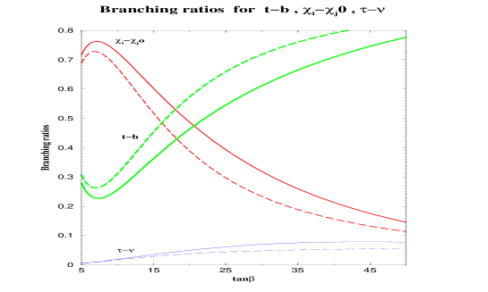
Figure 3: Plot of branching ratios for the decay of $H^{\pm}$ as a function of $\tan\beta$. The parameters are $m_{A}=800$, $m_{0}=400$, $m_{\frac{1}{2}}=140$, $A_{0}$=3, $\xi_{1}=0$, $\xi_{2}=0$, $\xi_{3}=0$, $\theta_{\mu}=0$, $\alpha_{A_{0}}=0$. The long dashed lines are the branching ratios at the tree level while the solid lines include the loop correction. The curves labelled $\chi_{i}^{-}\chi_{j}^{0}$ stand for sum of branching ratios into all allowed $\chi_{i}^{-}\chi_{j}^{0}$ modes. All masses are in unit of GeV and all angles in unit of radian. From Ref.(7).

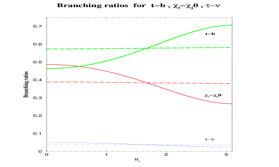
Figure 4: Plot of branching ratios for the decay of $H^{\pm}$ as a function of $\theta_{\mu}$ as a function of $\alpha_{A_{0}}$ in (b). The parameters are $m_{A}=800$, $m_{0}=400$, $m_{\frac{1}{2}}=140$, $A_{0}$=3, $\tan\beta=20$, $\xi_{1}=0$, $\xi_{2}=0$, $\xi_{3}=0$, $\theta_{\mu}=0$, $\alpha_{A_{0}}=0$. The long dashed lines are the branching ratios at the tree level while the solid lines include the loop correction. All masses are in unit of GeV and all angles in unit of radian. From Ref.(7).

4 Sizes of Loop Corrections

The theoretical analysis of effective Lagrangian obtained here including loop corrections is quite general. However, the parameter space of the general MSSM is quite large and thus we investigate the sizes of the effects in more constrained parameter space. This more constrained parameter space is provided by the extended SUGRA model. Thus we assume that the parameter space of the model to consist of $m_{A}$ (mass of the CP odd Higgs boson), $\tan\beta$, complex trilinear coupling $A_{0}$, $SU(3)$, $SU(2)$ and $U(1)_{Y}$ gaugino masses $\tilde{m}_{i}=m_{\frac{1}{2}}e^{i\xi_{i}}$ (i=1,2,3) and $\theta_{\mu}$, where $\theta_{\mu}$ is the phase of $\mu$. In the analysis the soft parameters are evolved from the grand unification scale to the electroweak scale. Further, as is usually the case the $\mu$ parameter is determined by the constraint of electroweak symmetry breaking while the phase of $\mu$, i.e,, $\theta_{\mu}$ remains an arbitrary parameter. It should be noted that while there are several phases in the analysis not all of them are independent[21].

The main modes of decay of the charged Higgs consist of final states which include top-bottom, chargino-neutralino ,and tau-neutrino . In Fig. 3 we give a plot of the branching ratios of $H^{-}$ to $\bar{t}b$, $\tau^{-}\bar{\nu}_{\tau}$ and $\chi_{i}^{-}\chi_{j}^{0}$ as a function of $\tan\beta$. For comparison the tree level branching ratio and the loop corrected branching ratios are plotted. The analysis of Fig. 3 shows that the loop corrections can be substantial and can reach as much as 20% or more. In Fig. 4 an analysis of the branching ratios for top-bottom, chargino-neutralino ,and tau-neutrino as a function of $\theta_{\mu}$ is given with and without loop corrections. The plots are given as a function of the $\mu$ phase. One finds that while the tree level analysis is independent of the phases the loop corrected branching ratios show a rather large dependence. The analysis illustrates both the importance of the loop corrections as well as dependence on the phases. Also of interest is the phenomenon of trileptonic signal arising from the decay of $H^{\pm}$. This arises when $H^{\pm}$ decays into a $\chi^{\pm}_{1}\chi_{2}^{0}$ with subsequent decays of $\chi^{-}_{1}$ and $\chi_{2}^{0}$ can provide a trileptonic mode. Thus, e.g., $H^{-}\rightarrow\chi^{-}_{1}\chi_{2}^{0}$ $\rightarrow$ ${\it l_{1}^{-}{\it l_{2}^{+}}{\it l}_{2}^{-}}$. Such a signal is well known in the context of the decay of the W boson. For off shell decays it was discussed in Ref.[22]. (For a more recent analysis see Ref.[23]). For the Higgs decay here, the signal can appear for on shell decays since the mass of the Higgs is expected to be large enough for such a decay to occur on shell. The analysis presented here shows that the effect of the loop corrections and of the CP phase $\theta_{\mu}$ on these signals can be substantial. The effect of other CP phases, e.g., $\xi_{3}$, $\alpha_{A}$ on the couplings and on the branching ratios can also be significant[20]. .

5 Conclusion

In this paper we have discussed the effective Lagrangian at the one loop level for the charged higgs-chargino-neutralino interactions. This analysis augments the previous such analyses for the $H^{+}\bar{t}b$ and $H^{+}\tau\bar{\nu}$ type couplings. The analysis presented here includes the dependence of the couplings on the supersymmetric CP phases. One of the interesting results of the analysis is the phenomenon that the supersymmetric loop corrections are generally quite substantial ,as much as 20-30% in significant regions of the parameter space of the theory. We also analysed in this paper the effects of the loop corrections on the decays of the charged Higgs. Specifically the analysis of the decay $H^{-}\rightarrow\chi_{1}^{-}\chi_{2}^{0}\rightarrow l_{1}^{-}l_{2}^{-}l_{2}^{+}$, which is the well known trileptonic signal, shows that the loop effects here are significant reaching as high as 20-30%. Finally it is found that the loop corrected couplings are quite sensitive to CP phases. The effective Lagrangian presented here should be of considerable interest in the analysis of charged Higgs decays and for the search for supersymmetry.

Acknowledgments
This research was also supported in part by NSF grant PHY-0139967.

References

[1]
For a recent review, see, M. Carena and H. E. Haber,
Prog. Part. Nucl. Phys. 50, 63 (2003) [arXiv:hep-ph/0208209].
[2]
M. Carena, D. Garcia, U. Nierste and C. E. M. Wagner,
Nucl. Phys. B 577, 88 (2000) [arXiv:hep-ph/9912516].
[3]
E. Christova, H. Eberl, W. Majerotto and S. Kraml,
JHEP 0212, 021 (2002) [arXiv:hep-ph/0211063]; E. Christova, H. Eberl, W. Majerotto and S. Kraml,
Nucl. Phys. B 639, 263 (2002) [Erratum-ibid. B 647, 359 (2002)] [arXiv:hep-ph/0205227].
[4]
T. Ibrahim and P. Nath,
Phys. Rev. D 67, 095003 (2003) [Erratum-ibid. D 68, 019901 (2003)] [arXiv:hep-ph/0301110].
[5]
T. Ibrahim and P. Nath,
Phys. Rev. D 68, 015008 (2003) [arXiv:hep-ph/0305201].
[6]
T. Ibrahim and P. Nath,
Phys. Rev. D 69, 075001 (2004) [arXiv:hep-ph/0311242].
[7]
A. H. Chamseddine, R. Arnowitt and P. Nath,
Phys. Rev. Lett. 49, 970 (1982)
:
R. Barbieri, S. Ferrara and C. A. Savoy,
Phys. Lett. B 119, 343 (1982)
.
For a review see, P. Nath,
arXiv:hep-ph/0307123.
[8]
E. Commins, et. al., Phys. Rev. A50, 2960(1994).
[9]
P.G. Harris et.al., Phys. Rev. Lett. 82, 904(1999).
[10]
S. K. Lamoreaux, J. P. Jacobs, B. R. Heckel, F. J. Raab and E. N. Fortson,
Phys. Rev. Lett. 57, 3125 (1986).
[11]
P. Nath, Phys. Rev. Lett.66, 2565(1991); Y. Kizukuri and N. Oshimo, Phys.Rev.D46,3025(1992).
[12]
T. Ibrahim and P. Nath, Phys. Lett. B 418, 98 (1998);
Phys. Rev. D57, 478(1998); Phys. Rev. D58, 111301(1998);
T. Falk and K Olive, Phys. Lett. B 439, 71(1998);
M. Brhlik, G.J. Good, and G.L. Kane, Phys. Rev. D59, 115004
(1999); A. Bartl, T. Gajdosik, W. Porod, P. Stockinger and H. Stremnitzer,
Phys. Rev. 60, 073003(1999);
S. Pokorski, J. Rosiek and C.A. Savoy,
Nucl.Phys. B570, 81(2000);
E. Accomando, R. Arnowitt and B. Dutta,
Phys. Rev. D 61, 115003 (2000);
U. Chattopadhyay, T. Ibrahim, D.P. Roy, Phys.Rev.D64:013004,2001;
M. Brhlik, L. Everett, G. Kane and J. Lykken, Phys. Rev.
Lett. 83, 2124, 1999;
T. Ibrahim and P. Nath, Phys. Rev. D61, 093004(2000).
[13]
T. Falk, K.A. Olive, M. Prospelov, and R. Roiban, Nucl. Phys.
B560, 3(1999);
V. D. Barger, T. Falk, T. Han, J. Jiang, T. Li
and T. Plehn,
Phys. Rev. D 64, 056007 (2001);
S.Abel, S. Khalil, O.Lebedev, Phys. Rev. Lett. 86, 5850(2001);
T. Ibrahim and P. Nath,
Phys. Rev. D 67, 016005 (2003) arXiv:hep-ph/0208142.
[14]
D. Chang, W-Y.Keung,and A. Pilaftsis, Phys. Rev. Lett. 82, 900(1999).
[15]
A. Pilaftsis, Phys. Rev. D58, 096010; Phys. Lett.B435, 88(1998); A. Pilaftsis and C.E.M. Wagner, Nucl. Phys. B553, 3(1999);
D.A. Demir, Phys. Rev. D60, 055006(1999); S. Y. Choi, M. Drees and J. S. Lee,
Phys. Lett. B 481, 57 (2000); T. Ibrahim and P. Nath, Phys.Rev.D63:035009,2001; hep-ph/0008237; T. Ibrahim,
Phys. Rev. D 64, 035009 (2001);
T. Ibrahim and P. Nath,
Phys. Rev. D 66, 015005 (2002);
S. W. Ham, S. K. Oh, E. J. Yoo, C. M. Kim and D. Son,
arXiv:hep-ph/0205244; M. Boz,
Mod. Phys. Lett. A 17, 215 (2002).
; M. Carena, J. R. Ellis, A. Pilaftsis and C. E. Wagner,
Nucl. Phys. B 625, 345 (2002) [arXiv:hep-ph/0111245].
: J. Ellis, J. S. Lee and A. Pilaftsis,
arXiv:hep-ph/0404167.
[16]
U. Chattopadhyay, T. Ibrahim and P. Nath,
Phys. Rev. D60,063505(1999);
T. Falk, A. Ferstl and K. Olive, Astropart. Phys. 13, 301(2000);
K. Freese and P. Gondolo, hep-ph/9908390;
[17]
M. E. Gomez, T. Ibrahim, P. Nath and S. Skadhauge,
Phys. Rev. D 70, 035014 (2004)
[arXiv:hep-ph/0404025].
;
arXiv:hep-ph/0410007.
[18]
For a more complete set of references see, T. Ibrahim and P. Nath, “Phases and CP violation in SUSY,” arXiv:hep-ph/0210251 published in P. Nath
and P. M. . Zerwas, “Supersymmetry and unification of fundamental interactions. Proceedings, 10th International Conference, SUSY’02, Hamburg,
Germany, June 17-23, 2002,” DESY-PROC-2002-02
[19]
J. A. Grifols and A. Mendez,
Phys. Rev. D 22, 1725 (1980).
[20]
T. Ibrahim, P. Nath and A. Psinas,
Phys. Rev. D 70, 035006 (2004)
[arXiv:hep-ph/0404275].
[21]
T. Ibrahim and P. Nath,
Phys. Rev. D 58, 111301 (1998) [arXiv:hep-ph/9807501].
[22]
P. Nath and R. Arnowitt,
Mod. Phys. Lett. A 2, 331 (1987).
[23]
For a recent update see, H. Baer, T. Krupovnickas and X. Tata,
JHEP 0307, 020 (2003) [arXiv:hep-ph/0305325];
For a review and a more complete set of references, see S. Abel et al. [SUGRA Working Group Collaboration],
arXiv:hep-ph/0003154.