Physics Beyond the Standard Model: Focusing on the Muon Anomaly

Abstract

We present a model based on the implication of an exceptional $E_{6}$-GUT symmetry for the anomalous magnetic moment of the muon. We follow a particular chain of breakings with Higgses in the $\mathbf{78}$ and $\mathbf{351}$ representations. We analyse the radiative correction contributions to the muon mass and the effects of the breaking of the so-called Weinberg symmetry. We also estimate the range of values of the parameters of our model.

1 Introduction

Among the known leptons, the muon is potentially interesting for several reasons. First, its relatively long lifetime of 2.2 $\mu$s $(c\tau=658.65\ m)$ makes it possible to perform precision measurements. Second, it is sensitive to new sectors of heavy particles and new interactions. In this sense, the muon anomaly has provided a stringent test for new theories of Particle Physics, since any new field or particle which couples to the muon must contribute to $a_{\mu}$.

The most recent results reported by the Muon $(g-2)$ Collaboration [1] have triggered a renewal of interest on the theoretical prediction of the anomalous magnetic moment of the muon (commonly referred to as the muon anomaly), $a_{\mu}=\frac{g-2}{2}$, in the Standard Model (SM). This experimental value is claimed  to show that there remains a discrepancy with the SM theoretical calculations at the confidence level of $2.3\sigma$ to $3.3\sigma$ [1][2], if the hadronic light-by-light contribution, $a_{\mu}^{HHO}(LBL)=80(40)\times 10^{-11}\cite[cite]{[\@@bibref{}{3}{}{}]}$, is used instead of $a_{\mu}^{HHO}(LBL)=136(25)\times 10^{-11}\cite[cite]{[\@@bibref{}{4}{}{}]}$, as a consequence that $e^{+}e^{-}$ annihilation data are used to evaluate this contribution against hadronic $\tau$ decays data [5]. Among all contributions that yield corrections to the muon anomaly, the hadronic contributions are less accurate, due to the hadronic vacuum polarization effects in the diagrams which use data inputs coming from the $e^{+}e^{-}$ annihilation cross section and the hadronic $\tau-$ decays. Also it is not clear, at present, whether the value from $\tau-$ decay data can be improved much further, due to the difficulty in evaluating more precisely the effect of isospin breaking [5].

In fact, these measurements have provided the highest accuracy of the validity of the different theories for strong, weak and electromagnetic interactions because they have reached a fabulous relative precision of 0.5 parts per million (ppm) in the determination of $a_{\mu}$. However, if this confidence level for the muon anomaly remains, it is possible that we are under a window open for a New Physics at a high energy scale, $\Lambda.$ The study of the muon anomaly becomes relevant because it is more sensitive to interactions that are not predicted in the SM but will be possibly reached at the CERN Large Hadron Collider (LHC), with $\sqrt{s}=14\,TeV$ .

On the theoretical side, if we take into account the effects of virtual massive particles in the diagrams contributing to the lepton anomaly, the ratios between the corrections to the anomalies are of the order $\Big{(}{\frac{m_{\mu}}{m_{e}}}\big{)}^{2}\sim 4\times 10^{4}$ for the muon and electron, and of the order $\Big{(}{\frac{m_{\tau}}{m_{e}}}\Big{)}^{2}\sim 1.2\times 10^{7}$ for the tau and electron. The same huge enhancement factor would also affect the contributions coming from degrees of freedom beyond the SM, so that the measurement of the $\tau-$ anomaly would represent the best opportunity to detect new physics. Unfortunately, the very short lifetime of the $\tau$- lepton which, precisely because of its high mass, can also decay into hadronic states, makes such a measurement impossible at present; this is the reason why there is an emphasis on the muon anomaly.

In this case, it becomes interesting to estimate the order of the correction of $a_{\mu}$ in the context of theories beyond the SM. This is done in terms of powers of $\frac{m_{\mu}}{\Lambda}$. This is related [10] to the validity or the breaking of the chiral symmetry for leptons together with the change of sign for $m_{\mu}$. If this symmetry, which is referred to as Weinberg Symmetry (WS), is respected, then $\Delta a_{\mu}\sim\left(m_{\mu}/\Lambda\right)^{2}$; on the other hand, if it is broken, $\Delta a_{\mu}\sim m_{\mu}/\Lambda$ . This is important because in the latter case the explanation of the muon anomaly may be given by a new physics at a relatively high energy, whereas in the former it should appear at a scale close to the electroweak (EW) one.

We consider the 78 and 351 Higgs representations of THE $E_{6}$ Grand-Unified Theory (GUT). The representations between square brackets refer to the $E_{6}$-group, those between brackets refer to $SO(10)\otimes\bar{U}(1)$ and the ones between parentheses correspond to the $SU(5)\otimes\tilde{U}(1)$ group. The symmetry breaking pattern [6, 7, 8, 9] is depicted below.

$$\begin{array}[c]{c}E_{6}\\ [\mathbf{78]}\left\{\mathbf{1,0}\right\}\\ \downarrow\end{array}$$

$$\begin{array}[c]{c}SO(10)\otimes\overline{U}(1)\\ [\mathbf{351]}\left\{\mathbf{1,-8}\right\}\\ \downarrow\end{array}$$

$$\begin{array}[c]{c}SO(10)\\ [\mathbf{78]}\left\{\mathbf{45,0}\right\}(\mathbf{1,0)}\\ \downarrow\end{array}$$

$$\begin{array}[c]{c}SU(5)\otimes\widetilde{U}(1)\\ [\mathbf{351]}\left\{\mathbf{16,-5}\right\}(\mathbf{1,-5)}\\ \downarrow\end{array}$$ (1)

$$\begin{array}[c]{c}SU(5)\\ \begin{array}[]{ll}{[\mathbf{351]}\left\{\mathbf{54,4}\right\}(\mathbf{24,0),}}\\ {[\mathbf{351]}\left\{\mathbf{144,1}\right\}(\mathbf{24,5)}}\end{array}\\ \downarrow\end{array}$$

$$\begin{array}[c]{c}SU(3)_{C}\otimes SU(2)_{L}\otimes U(1)\\ [\mathbf{351]}\left\{\mathbf{10,-2}\right\}\\ \downarrow\end{array}$$

$$SU(3)_{C}\otimes U(1)_{e.m}$$

The order of magnitude of the contribution is $\Delta a_{\mu}\sim m_{\mu}/m_{M}$, where $m_{M}$ is the mass of the exotic fermion. This fermion is analogous to the ordinary muon contained in the $[\mathbf{27}]$ representation of fermions in $\{\mathbf{10},-2\}$ under $SO(10)\times\bar{U}(1)$. This connection makes sense if the radiative correction to the muon mass is small and if there occurs breaking of WS. On the other hand, if the muon mass is only due to radiative corrections, the right mixing angle between leptons is zero and WS is not broken.

Our paper is organized as follows. In the Section 2, we discuss the WS in the SM in connection with the order of magnitude of the muon anomaly. In the Section 3, we present our model, considering the sequences of breakings of symmetries (1). In Section 4, we analyse the question of the radiative mass of the muon due to the mixings with the massive fermion that occur in the breaking chain $SU(5)\longrightarrow SU(3)_{C}\otimes SU(2)_{L}\otimes U(1)$ with $\left\{\mathbf{144,1}\right\}$ Higgs; in Section 5, we analyse WS in the context of our model and, finally, in Section 6, we present our General Conclusions.

2 WS and the anomalous magnetic moment in the SM

The WS is a well-known property [10] of the SM of Particle Physics. In this section, we briefly review its main points, since this result is connected with the order of magnitude of the $\Delta a_{\mu}$ contribution in the $E_{6}$ model. The mass term $m_{\mu}\overline{\mu}\mu$ breaks chiral symmetry; the field redefinition below changes the sign of the mass term:

$${\Large\mu\rightarrow\gamma}_{5}{\Large\mu\quad,\quad m}_{\mu}{\Large\rightarrow-m}_{\mu}{\Large\,,}$$ (2)

where $\mu$ is the field variable associated to the muon.

If the WS Eq. (2) is valid, the corrections to $a_{\mu}$ must be of even powers of the ratio of $m_{\mu}$ to a larger scale $\Lambda:$

$${\Large a}_{\mu}{\Large=c}_{o}\left(\frac{m_{\mu}}{\Lambda}\right)^{0}{\Large+c}_{2}\left(\frac{m_{\mu}}{\Lambda}\right)^{2}{\Large+...\quad.}$$ (3)

The effective interaction that gives a non-zero contribution to the muon anomalous magnetic moment is $a_{\mu}\frac{e}{4m_{\mu}}\overline{\mu}\sigma_{{}_{\alpha\beta}}\mu F^{{}^{\alpha\beta}}$; for the SM version, it may be written as

$$\mathcal{L}_{\mathbf{eff}}\ {\Large=a}_{\mu}{\Large\,}\frac{e}{4m_{\mu}}\left(\overline{\Psi}_{L}\sigma^{\alpha\beta}\mu_{R}\frac{f_{0}\,\varphi_{V}}{m_{\mu}}+h.c.\right){\Large F}_{\alpha\beta}{\Large\quad,}$$ (4)

with a Higgs field doublet $\varphi=\left(\begin{array}[c]{c}0\\ \varphi_{1}\end{array}\right)=\varphi_{V}+\left(\begin{array}[c]{c}0\\ h_{1}/\sqrt{2}\end{array}\right)$ , such that

$$\overline{\Psi}_{L}\ {\Large=}\left(\begin{array}[c]{c}\nu\\ \mu\end{array}\right)_{L}{\Large\quad,\quad\varphi}_{V}\ {\Large=}\left(\begin{array}[c]{c}0\\ \frac{\upsilon_{1}}{\sqrt{2}}\end{array}\right){\Large\quad,\,\,}f_{0}\frac{\upsilon_{1}}{\sqrt{2}}\ {\Large=\ }m_{\mu}\,{\Large\,.}$$ (5)

Now, to have the WS invariance (2) in the SM, one must perform the transformations

$$\Psi_{L}{\Large\rightarrow\gamma}_{5}{\Large\,}\Psi_{L}{\Large=-}\Psi_{L}{\Large\quad,\quad\mu}_{R}{\Large\rightarrow\gamma}_{5}{\Large\mu}_{R}{\Large=\mu}_{R}{\Large\quad,\quad\varphi\rightarrow-\varphi\ .}$$ (6)

We can prove that the neutral current Lagrangian density reads as

$$\mathcal{L}_{NC}=-e\overline{\mu}{\Large\gamma}^{\alpha}{\Large\mu A}_{\alpha}-\frac{g}{2\cos\theta_{W}}\overline{\mu}{\Large\gamma}^{\alpha}\left(\upsilon_{z}-a_{z}\gamma^{5}\right){\Large\mu Z}_{\alpha};$$ (7)

the charged current Lagrangian density is written as

$$\mathcal{L}_{CC}=\frac{g}{2\sqrt{2}}\left[\overline{\nu}_{\mu}{\Large\gamma}^{\alpha}\left(1-\gamma^{5}\right){\Large\mu W}_{\alpha}^{\left(+\right)}+\overline{\mu}{\Large\gamma}^{\alpha}\left(1-\gamma^{5}\right){\Large\nu}_{\mu}{\Large W}_{\alpha}^{\left(-\right)}\right]{\Large\ ,}$$ (8)

and the Yukawa sector

$$\mathcal{L}_{YUK}=-f_{0}\left(\overline{\mu}_{R}\varphi^{\dagger}\mu_{L}+\overline{\mu}_{L}\varphi\mu_{R}\right)=-\frac{1}{\sqrt{2}}f_{0}\left(\upsilon_{1}+h_{1}\right)\overline{\mu}\mu,$$ (9)

where $m_{\mu}=f_{0}\frac{\upsilon_{1}}{\sqrt{2}}$ is the muon mass and the interactions are invariant under the transformations of Eq.(6). Therefore, the corrections to $a_{\mu}$ are of the type of Eq.(3) with the EW scale, $\Lambda$. The first term is the electromagnetic contribution $c_{0}=\frac{\alpha}{2\pi}+...$, computed recently up to $(\alpha/\pi)^{5}$ [11]; the second term, $c_{2}\left(\frac{m_{\mu}}{\Lambda}\right)^{2}\sim a_{\mu}^{QED}\times 1,7\times 10^{-6}\simeq 2\times 10^{-9}$, corresponds to the weak contribution.

3 An  alternative E₆-model for the muon anomaly

The exceptional group $E_{6}$ [12] was proposed as an alternative to $SU(5)-$and $SO(10)-$models, and it is actually, in many aspects, the preferred gauge group for Grand Unification. In this section, let us discuss the pattern of breakings (1) based on the $[\mathbf{78]}$ and $[\mathbf{351]}$ representations. The ordinary fermions of the SM are contained in the $\left\{\mathbf{16},1\right\}\subset$ $\mathbf{27-}$ dimensional representation:

$$[\mathbf{27]=}\left\{\mathbf{16},1\right\}\oplus\left\{\mathbf{10},-2\right\}\oplus\left\{\mathbf{1},4\right\}.$$ (10)

There are $11$ additional fermions with respect to the SM fermions. For the first generation, these particles are:

$${\underbrace{\mathbf{\Psi}_{L}}_{\left\{\mathbf{1},4\right\}}}\oplus{\underbrace{{\underbrace{\left(\mathbf{D}^{C}\quad\mathbf{N\quad E}\right)_{L}}_{\left(\overline{\mathbf{5}},-2\right)}}\oplus{\underbrace{\left(\mathbf{D}\quad\mathbf{N}^{C}\mathbf{\quad E}^{C}\right)_{L}}_{\left(\mathbf{5},2\right)}}}_{\left\{\mathbf{10},-2\right\}}}.$$ (11)

The gauge bosons are contained in the adjoint $\mathbf{78-}$dimensional representation, that, with respect to $SO(10)\otimes\overline{U}(1)$, is decomposed as below:

$$[\mathbf{78]=}\left\{\mathbf{45},0\right\}\oplus\left\{\mathbf{16},-3\right\}\oplus\left\{\mathbf{1},0\right\}\oplus\left\{\overline{\mathbf{16}},3\right\}.$$ (12)

For the first generation, the exotic fermions of the $\mathbf{10}$ representation of $SO(10)$ can acquire mass from the Higgs $\{\mathbf{54},4\}$ of   the $[\mathbf{351]}$ representation of $E_{6}$, because $\{\mathbf{10\}\otimes}\{\mathbf{10\}=\{54\}\oplus\{45\}\oplus\{1\}}$ . The mass terms are of the type [13]

$$\varphi_{2}\left(\mathbf{54,24}\right)\left(D^{c}D-\frac{3}{2}E^{c}E-\frac{3}{2}N^{c}N\right).$$ (13)

In this same representation, $\{\mathbf{144,}1\}$, let us mix these fermions with the ordinary ones, because both components contain a $\mathbf{24}$ of $SU(5)$, which has one invariant component under $SU(3)_{C}\otimes SU(2)_{L}\otimes U(1)_{Y}$ : $\{\mathbf{16\}\otimes\{10\}=\{144\}\oplus\{}\overline{\mathbf{16}}\}.$ This mixing term is given by

$$\varphi_{3}\left(\mathbf{144,24}\right)\left(d^{c}D-\frac{3}{2}E^{c}e-\frac{3}{2}N^{c}\nu\right).$$ (14)

Observe that both Higges, $\varphi_{2}\left(\mathbf{54,24}\right)$ and $\varphi_{3}\left(\mathbf{144,24}\right)$, being singlets $\left(\mathbf{1,1,}0\right)$ under $SU(3)_{C}\otimes SU(2)_{L}\otimes U(1)_{Y}$, we shall assume that they take  diferent values of expectation around his quantum fields $h_{2}$ and $h_{3}$:

$$\varphi_{2}\left(\mathbf{54,24}\right) =\frac{1}{\sqrt{2}}\left(\upsilon_{2}+h_{2}\right)$$ (15)

$$\varphi_{3}\left(\mathbf{144,24}\right) =\frac{1}{\sqrt{2}}\left(\upsilon_{3}+h_{3}\right),$$ (16)

where the v.e.v’s $\upsilon_{3}$ and $\upsilon_{2}$ we will assume them to satisfy the relation $\upsilon_{3}\leq\upsilon_{2}.$

On the other hand, the ordinary fermions of the SM get masses from the Higgs $\left\{\mathbf{10},-2\right\}$, because the Yukawa term that conserves the $\overline{U}(1)$ charge is

$$\{\mathbf{16\}\otimes}\{\mathbf{16\}=}\{\mathbf{10\}\oplus}\{\mathbf{126\}\oplus}\{\mathbf{120\}},$$ (17)

and this Higgs is in the $[\mathbf{351].}$ This mass term is

$$H\left(\mathbf{10,}\overline{\mathbf{5}}\right)\left(d^{C}d+e^{C}e+N^{C}L\right).$$ (18)

In order to explain the notation, here $\varphi\,\acute{}\left(\mathbf{a,24}\right)$ stands for the component of the Higgs representation, $\varphi\,\acute{},$ where the label $\mathbf{a}$ indicates the transformation under $SO(10)$ and the label $\mathbf{24}$-component refers to $SU(5)$; similarly, for $H\left(\mathbf{10,}\overline{\mathbf{5}}\right).$ In fact, this Higgs $H\left(\mathbf{10,}\overline{\mathbf{5}}\right)$ is indeed that one of the SM $\varphi_{1}\left(\mathbf{1,2,}1/2\right)$ under $SU(3)_{C}\otimes SU(2)_{L}\otimes U(1)_{Y}$ which is, as we already said before, written as

$$\varphi_{1}\left(\mathbf{1,2,}1/2\right)=\frac{1}{\sqrt{2}}\left(\upsilon_{1}+h_{1}\right).$$ (19)

Now, let us extend this for the second generation of fermions, and call $M$ the supermassive fermion in analogy to the ordinary muon of the SM.

If the breakings of symmetry are due to a $[\mathbf{351]}$ , when the GUT symmetry is broken, the mass eigenstates $\mu_{o}$ and $\widehat{M}$ are determined by the expectation values of the $\left(SO(10),SU(5)\right)$ multiplets $\varphi_{2}\,\left(\mathbf{54,24}\right)$ and $\varphi_{3}\left(\mathbf{144,24}\right)$, through the mixture of left and right components [13][14]:

$$\left(\begin{array}[c]{c}{\Large\mu}_{L,R}\\ M_{L,R}\end{array}\right)=\left(\begin{array}[c]{cc}\cos{\Large\theta}_{L,R}&\sin{\Large\theta}_{L,R}\\ -\sin{\Large\theta}_{L,R}&\cos{\Large\theta}_{L,R}\end{array}\right)\left(\begin{array}[c]{c}{\Large\mu}_{L,R}^{0}\\ \widehat{M}_{L,R}\end{array}\right),$$ (20)

where $\theta_{L,R}$ are the left nd right mixing angles, respectively. It is possible that the mixing angle $\theta_{R}$ is small, of the order $\sim m_{\mu}/m_{M}$, where $m_{M}$ is the mass of the heavy muon, $M$, however, due to the weak universality, the angle $\theta_{L}$ between $\mu_{L}$ and $M_{L}$ is expected to be the same mixing angle for  $\nu^{\mu}$ and the neutral exotic lepton $N$; but $\theta_{L}$ can still be large [15].

The fermion-Higgs interaction Lagrangian is given by:

$$L=\frac{f_{0}}{\sqrt{2}}\overline{\mu_{L}}\mu_{R}\,(h_{1}+\upsilon_{1})+\frac{f_{1}}{\sqrt{2}}\overline{M_{L}}M_{R}\,(h_{2}+\upsilon_{2})+\frac{f_{2}}{\sqrt{2}}\overline{\mu_{L}}M_{R}\,(h_{3}+\upsilon_{3})+$$

$$\frac{f_{3}}{\sqrt{2}}\overline{M_{L}}\mu_{R}\,(h_{1}+\upsilon_{1})+h.c.,$$ (21)

where some of the $\ f_{i}\acute{}\,$s could be vanishing. The previous expression can be written as below:

$$L=\left(\begin{array}[c]{cc}\overline{\mu_{L}}&\overline{M_{L}}\end{array}\right)\frac{1}{\sqrt{2}}\left(\begin{array}[c]{cc}f_{0}\upsilon_{1}&f_{2}\upsilon_{3}\\ f_{3}\upsilon_{1}&f_{1}\upsilon_{2}\end{array}\right)\left(\begin{array}[c]{c}\mu_{R}\\ M_{R}\end{array}\right).$$ (22)

The mass matrix reads as:

$$\mathbf{M=}\frac{1}{\sqrt{2}}\left(\begin{array}[c]{cc}f_{0}\upsilon_{1}&f_{2}\upsilon_{3}\\ f_{3}\upsilon_{1}&f_{1}\upsilon_{2}\end{array}\right).$$ (23)

As usually, the previous matrix mass is diagonalized by a bi-unitary transformation [14] [16] $U_{L}^{\dagger}\mathbf{M}U_{R}=\mathbf{M}_{diag}$, where $U_{L,R}$ is given in (20). From $U_{L}^{\dagger}\mathbf{MM}^{\dagger}U_{L}=\mathbf{M}_{diag}^{2}\ ,$ it is possible to find

$$\tan\left(2\theta_{L}\right)=\frac{2\left(f_{0}f_{3}\upsilon_{1}^{2}+f_{1}f_{2}\upsilon_{2}\upsilon_{3}\right)}{\left(f\ _{3}^{2}-f\ _{0}^{2}\right)\upsilon_{1}^{2}+f\ _{1}^{2}\upsilon_{2}^{2}-f\ _{2}^{2}\upsilon_{3}^{2}}\ ;$$ (24)

on the other hand, from $U_{R}^{\dagger}\mathbf{M}^{\dagger}\mathbf{M}U_{R}=\mathbf{M}_{diag}^{2}$ , we obtain

$$\tan\left(2\theta_{R}\right)=\frac{2\left(f_{0}f_{2}\upsilon_{1}\upsilon_{3}+f_{1}f_{3}\upsilon_{1}\upsilon_{2}\right)}{f\ _{1}^{2}\upsilon_{2}^{2}+f\ _{2}^{2}\upsilon_{3}^{2}-\left(f\ _{3}^{2}+f\ _{0}^{2}\right)\upsilon_{1}^{2}}\ .$$ (25)

In the limit for which all the couplings $f_{i}$ are equal and $\upsilon_{3}\simeq\upsilon_{2}\gg\upsilon_{1}$, we heve to $\tan\left(2\theta_{L}\right)\rightarrow\infty$,

$$\tan\left(2\theta_{R}\right)\simeq\frac{2\upsilon_{1}\upsilon_{2}}{\upsilon_{2}^{2}-\upsilon_{1}^{2}}$$ (26)

or to the algles $\theta_{L}$ and $\theta_{R}$ the values $\theta_{L}=\frac{\pi}{4}$ , $\theta_{R}\sim\frac{\upsilon_{1}}{\upsilon_{2}}$. As it can be seen, in this case $\theta_{R}$ is small.

The part of the interaction Lagrangian for the quantum flutuations can be written as:

$$L=\frac{f_{0}}{\sqrt{2}}\overline{\mu_{L}}\mu_{R}\,h_{1}+\frac{f_{1}}{\sqrt{2}}\overline{M_{L}}M_{R}\,h_{2}+\frac{f_{2}}{\sqrt{2}}\overline{\mu_{L}}M_{R}\,h_{3}+\frac{f_{3}}{\sqrt{2}}\overline{M_{L}}\mu_{R}\,h_{1}+h.c.;$$ (27)

after the mixing equations (20), we obtain the changing-flavor Lagrangian:

$$L_{FC}=\frac{f_{0}}{\sqrt{2}}(c_{L}s_{R}\overline{\mu_{L}^{0}}\widehat{M}_{R}+c_{R}s_{L}\overline{\widehat{M}_{L}}\,\mu_{R}^{0})h_{1}+\frac{f_{1}}{\sqrt{2}}(-s_{L}c_{R}\overline{\mu_{L}^{0}}\widehat{M}_{R}-c_{L}s_{R}\overline{\widehat{M}_{L}}\,\mu_{R}^{0})\,h_{2}+$$ (28)

$$\frac{f_{2}}{\sqrt{2}}(c_{R}c_{L}\overline{\mu_{L}^{0}}\widehat{M}_{R}-s_{L}s_{R}\,\overline{\widehat{M}_{L}}\,\mu_{R}^{0})h_{3}+\frac{f_{3}}{\sqrt{2}}(-s_{L}s_{R}\overline{\mu_{L}^{0}}\widehat{M}_{R}+c_{L}c_{R}\overline{\widehat{M}_{L}}\,\mu_{R}^{0})\,h_{1}+h.c.$$

where $c_{L,R}=\cos\theta_{L,R}$ and $s_{L,R}=\sin\theta_{L,R}$ . We label the neutral mass eigenstates of the Higgses by $H_{1},H_{2},H_{3}$ whose masses are $M_{1},M_{2},M_{3}$ respectively. Then, suitable rotations between of fields $h_{1},h_{2},h_{3}$ must diagonalize the mass matrix in the potential $V(h_{1},h_{2},h_{3}).$ We suppose (from now in ahead) that $M_{1}\ll M_{3}\simeq M_{2},$ assuming conservation of CP, the matrix of rotations will be real. In the limit $\upsilon_{1}\ll\upsilon_{3}\leq\upsilon_{2}$, the state $h_{1}\longrightarrow H_{1}$ is weak and any appreciable mixing between scalars will only appear between $h_{2}$ and $h_{3}:$

$$\left(\begin{array}[c]{c}h_{2}\\ h_{3}\end{array}\right)=\left(\begin{array}[c]{cc}\cos\vartheta&-\sin\vartheta\\ \sin\vartheta&\cos\vartheta\end{array}\right)\left(\begin{array}[c]{c}H_{2}\\ H_{3}\end{array}\right),$$ (29)

with $\vartheta$ being the angle of rotation that allows the diagonalization of the matrix. With these mixings of neutral scalars fields, the flavor-changing Lagrangian (28) now takes the form:

$$L_{FC}^{eff}=\frac{1}{2\sqrt{2}}{\displaystyle\sum\limits_{i=1}^{3}}\overline{\mu^{0}}\left[\widetilde{\beta}_{i}+\widetilde{\alpha}_{i}-\gamma_{5}(\widetilde{\beta}_{i}-\widetilde{\alpha}_{i})\right]\widehat{M}H_{i}+h.c.,$$ (30)

where

$$\widetilde{\alpha}_{1}=f_{0}c_{L}s_{R}-f_{3}s_{L}s_{R},$$

$$\widetilde{\beta}_{1}=f_{0}c_{R}s_{L}+f_{3}c_{L}c_{R},$$

$$\widetilde{\alpha}_{2}=-f_{1}c_{R}s_{L}\cos\vartheta+f_{2}c_{R}c_{L}\sin\vartheta$$

$$\widetilde{\beta}_{2}=-f_{1}c_{L}s_{R}\cos\vartheta-f_{2}s_{L}s_{R}\sin\vartheta,$$ (31)

$$\widetilde{\alpha}_{3}=f_{1}c_{R}s_{L}\sin\vartheta+f_{2}c_{L}c_{R}\cos\vartheta,$$

$$\widetilde{\beta}_{3}=f_{1}c_{L}s_{R}\sin\vartheta-f_{2}s_{L}s_{R}\cos\vartheta.$$

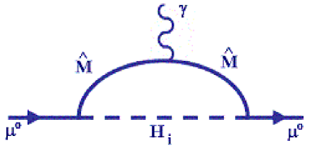
Figure 1: Contributions  with Higgs-interchange to the muon anomalous magnetic moment.

The generic diagram with Higgs interchange contributing to the anomaly of the muon is shown in Fig.1. In fact, the explicit calculation [17] of the one-loop contribution yielded by Eq. (29) gives the results (in the limit $m_{M}/m_{\mu}\gg 1$) :

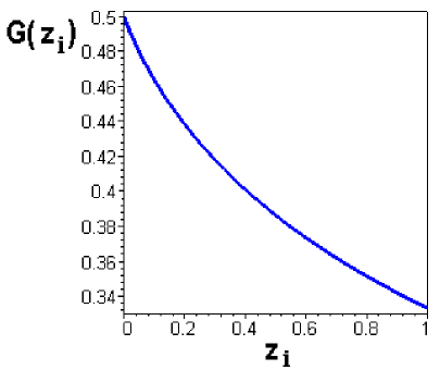
Figure 2: Plot of $G(z_{i})$ as function of $z_{i},$ where $z_{i}=M_{i}^{2}/m_{M}^{2}$ .

$${\Large\Delta a}_{\mu}^{FCh}\ =\frac{1}{128\pi^{2}}m_{\mu}^{2}\sum_{i=1}^{3}\xi_{i}^{2}{\displaystyle\int\limits_{0}^{1}}dx\frac{\left(x^{2}-x^{3}\right)+\frac{m_{M}}{m_{\mu}}x^{2}}{m_{\mu}^{2}x^{2}+\left(m_{M}^{2}-m_{\mu}^{2}\right)x+M_{i}^{2}\left(1-x\right)}=$$

$$={\Large\ }\frac{1}{128\pi^{2}}\frac{m_{\mu}}{m_{M}}\sum_{i=1}^{3}\xi_{i}^{2}G(z_{i}){\Large\quad,}$$ (32)

denoting $\ z_{i}=\frac{M_{i}^{2}}{m_{M}^{2}}$ where $\ \xi_{i}^{2}=$ $\alpha_{i}^{2}-\beta_{i}^{2}$ with  $\alpha_{i}=\widetilde{\beta}_{i}+\widetilde{\alpha}_{i}$ , $\beta_{i}=\widetilde{\beta}_{i}-\widetilde{\alpha}_{i}$ the function $G(z_{i})=\frac{\left(1-z_{i}\right)^{2}-2z_{i}\left(1-z_{i}\right)-2z_{i}^{2}\ln z_{i}}{2\left(1-z_{i}\right)^{3}}$ is plotted in Fig. (2). Let us see two cases of interest:

a) $m_{M}\simeq M_{2}\simeq M_{3}\gg M_{1}$ . If we consider the rough case in that $f_{1}=f_{2}$ , we have $\xi_{3}^{2}=\xi_{2}^{2}$ with the reasonable value $G\left(z_{2,3}\right)\simeq 0.3$ and $G\left(z_{1}\right)\simeq 0.5$ In this case the total contribution is

$${\Large\Delta a}_{\mu}^{FCh}\ =\frac{1}{128\pi^{2}}\frac{m_{\mu}}{m_{M}}(0.5\times\xi_{1}^{2}+0.6\times\xi_{2}^{2})\quad,$$ (33)

then, for to complete the anomaly value [2] ${\Large\Delta a}_{\mu}=25.2\times 10^{-10},$ we have

$$7.4\times 10^{-3}\leq\xi_{1}^{2}+1.2\times\xi_{2}^{2}\leq 0.64$$ (34)

where we consider $115\,GeV\leq m_{M}\leq 10\,TeV.$

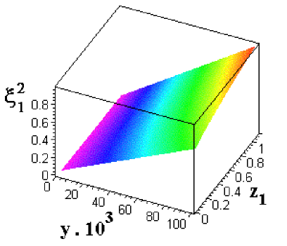
Figure 3: Space of values of $\xi_{1}^{2}$ in the range of masses $115\,GeV\leq m_{M}\leq 10TeV,$ $115\,GeV\leq M_{1}\leq 700$ GeV for to complate the anomaly value, where $y=\frac{m_{M}}{m_{\mu}}.$

b) $M_{2}\simeq M_{3}\gg M_{1}\simeq m_{M}.$ The principal contribution come from $H_{1}$

$${\Large\Delta a}_{\mu}^{FCh}\ (H_{1})\simeq\frac{1}{128\pi^{2}}\frac{m_{\mu}}{m_{M}}\xi_{1}^{2}\ G(z_{1})\,,$$ (35)

and this case $G(z_{2,3})\longrightarrow 0.$ We can find the limits of $\xi_{1}^{2}$ over the range masses indicated $7\times 10^{-3}\leq\xi_{1}^{2}\ \leq 0.61,$ as illustred in Fig. 3.

4 Radiative corrections to the muon mass

Other interesting possibility is to suppose a situation in which the muon mass comes only from radiative corrections. There are models of this type [19] [20] in the literature. In the Ref. [20], the authors, working out an $SU(3)\otimes SU(3)\otimes U(1)$ model, introduce some symmetries to avoid  the light fermions from acquiring their masses at tree-level through their couplings to the SM Higgs boson with non-zero vacuum expectation value; as a consequence, the muon gets its mass from the radiative corrections induced by other particles.

The one-loop correction to the muon mass is obtained by removing the photon line from the diagram Fig.(1). The amplitude for this diagram is:

$$\Sigma\left(p\right) =-i\kappa^{2}\Big{[}\int\frac{d^{4}q}{\left(2\pi\right)^{4}}\frac{m_{M}\left(\left|\alpha_{i}\right|^{2}-\left|\beta_{i}\right|^{2}\right)+\left(\left|\alpha_{i}\right|^{2}+\left|\beta_{i}\right|^{2}\right)\gamma^{\mu}q_{\mu}}{\left(q^{2}-m_{M}^{2}\right)\left((p-q)^{2}-M_{i}^{2}\right)}+$$ (36)

$$+\int\frac{d^{4}q}{\left(2\pi\right)^{4}}\frac{+(\alpha_{i}\beta_{i}^{\dagger}+\beta_{i}\alpha_{i}^{\dagger})q_{\mu}\gamma^{\mu}\gamma_{5}+m_{M}(\alpha_{i}\beta_{i}^{\dagger}-\beta_{i}\alpha_{i}^{\dagger}\,)\gamma_{5}}{\left(q^{2}-m_{M}^{2}\right)\left((p-q)^{2}-M_{i}^{2}\right)}\Big{]},$$

where $\kappa=\frac{1}{2\sqrt{2}}$ and $\ i=1,2,3.$ Let us suppose that $M_{2}$ is the maximal energy scale for our model, then, as $m_{\mu}\ll m_{M},M_{2}$, we obtain the folowing expression for the radiately induced muon mass:

$$m_{\mu}^{\mbox{1-loop}}=\frac{\left(\alpha_{2}^{2}-\beta_{2}^{2}\right)}{8\left(4\pi\right)^{2}}m_{M}F\left(z_{2}\right),$$ (37)

$$F\left(z_{2}\right)=1-\frac{1}{z_{2}-1}\ln z_{2},$$ (38)

where $z_{2}=$ $\frac{M_{2}^{2}}{m_{M}^{2}}.$ Notice that, for $M_{2}\simeq M_{3}\gg m_{M},M_{1}$ (or $z_{2,3}\gg 1)$, the function $F\left(z_{2}\right)$ takes it asymptotic value equal to 1, then

$$m_{\mu}^{\mbox{loop}}(H_{2},H_{3})\simeq\frac{\xi_{2}^{2}}{128\pi^{2}}m_{M},$$ (39)

and for the case $M_{2}\simeq M_{3}\simeq m_{M}\gg M_{1}$ the function $F\left(z_{2}\right)\simeq 1-m_{M}^{2}/M_{2}^{2}.$ To assure small radiative mass for the muon, for example of $\ 0.1$ $MeV-10\,MeV$  with $115\,GeV\leq m_{M}\leq 10\,TeV,$ it is necessary that $1.0\times 10^{-3}\leq\xi_{2}^{2}\leq 1.3\times 10^{-3}.$

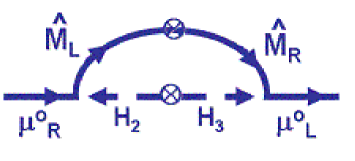
Figure 4: Diagram of radiative correction to muon mass with mixing bettween heavy scalar.

There is another diagram that can contribute to the radiative mass of the muon, as it is shown in Fig. 4. The result was estimated [18] [20] as

$$m_{\mu}^{\mbox{1-loop}}\simeq\frac{\varepsilon}{16\pi^{2}}m_{M}\left[\frac{M_{2}^{2}}{m_{M}^{2}-M_{2}^{2}}\ln\left(\frac{m_{M}^{2}}{M_{2}^{2}}\right)-\frac{M_{3}^{2}}{m_{M}^{2}-M_{3}^{2}}\ln\left(\frac{m_{M}^{2}}{M_{3}^{2}}\right)\right]\,,$$ (40)

where $\varepsilon$ is an parameter function of Yukawa couplings that (can read from (29) and (30)) and of the mixing angle $\vartheta.$ However, $\widehat{M},$ $H_{2}$ and $H_{3}$ for the limit natural $m_{M}\ll M_{2}\simeq M_{3}$ , $m_{\mu}^{\mbox{1-loop}}$ is essentially zero.

In our model, the ordinary fermions are massles at the tree level in the GUT scale (i.e no bare $m_{\mu}^{\mbox{o}}$  is possible due to symmetry), but it couples to the heavy fermion $\widehat{M}$  through the mixing with scalars, according to the breaking $SU(5)\otimes\widetilde{U}(1)\longrightarrow SU(5)$. If we suppose this, then the only diagrams that contribute to the anomaly are those with the interchange of $H_{2}$ and $H_{3}$ in the Fig. (1). To simplify, let us suppose the case $M_{2}\simeq M_{3}$ and $f_{1}=f_{2}$ from which $\xi_{2}^{2}=\xi_{3}^{2}$; then, the contribution with the $H_{2}$-interchange is

$$\Delta a_{\mu}^{FCh}=\frac{\xi_{2}^{2}}{128\pi^{2}}\frac{m_{\mu}}{m_{M}}G\left(z_{2}\right);$$ (41)

but, from (36) and (37), we can write for $M_{2}\gg m_{M}$

$$m_{\mu}^{\mbox{1-loop}}\simeq\frac{\xi_{2}^{2}}{128\pi^{2}}m_{M}F(z_{2});$$ (42)

combining these equations, we obtain

$$\Delta a_{\mu}^{FCh}\simeq\frac{m_{\mu}^{2}}{M_{2}^{2}}\times\frac{z_{2}[(1-z_{2})^{2}-2z_{2}\left(1-z_{2}\right)+2z_{2}^{2}\ln z_{2})}{2(1-z_{2})^{3}},$$ (43)

where the function $P(z_{2})=\frac{z_{2}[(1-z_{2})^{2}-2z_{2}\left(1-z_{2}\right)+2z_{2}^{2}\ln z_{2})}{2(1-z_{2})^{3}}$ is plotted in the Fig.5.  In this way, if the mass of the muon is of radiative origin we obtain $\Delta a_{\mu}^{FCh}\sim m_{\mu}^{2}/M_{2}^{2}$ . An analogous result was obtained by Marciano using a toy model [21] .

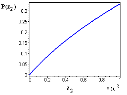
Figure 5: Plot of $P(z_{2})$ . Note that $P(z_{2})$ is roughly $\mathcal{O(}1\mathcal{)}$ on the values range considered.

5 Weinberg symmetry invariance

In terms of the mixing angles $\theta_{L,R}$

, from the bi-unitary diagonalization $U_{L}^{\dagger}\mathbf{M}U_{R}=\mathbf{M}_{\mathbf{diag}}$, we find for the masses

$$m_{\mu} =\frac{1}{\sqrt{2}}[(c_{L}f_{0}-s_{L}f_{3})\upsilon_{1}c_{R}-(c_{L}f_{2}\upsilon_{3}-s_{L}f_{1}\upsilon_{2})s_{R}],$$ (44)

$$m_{M} =\frac{1}{\sqrt{2}}[(s_{L}f_{0}+c_{L}f_{3})\upsilon_{1}s_{R}+(s_{L}f_{2}\upsilon_{3}+c_{L}f_{1}\upsilon_{2})c_{R}],$$ (45)

where $\theta_{L,R}$ are given in (24) and (25), respectively. Under the WS in (6): $\varphi\longrightarrow-\varphi$ , (equivalently $\upsilon_{1}\longrightarrow-\upsilon_{1}\,$), $\theta_{L}$ is invariant, but $\theta_{R}\longrightarrow-\theta_{R}$, then $m_{\mu}\longrightarrow-\,m_{\mu}$ and $m_{M}$ is invariant $m_{M}\rightarrow m_{M},$. Now, let us remember that $\mu$ and $M$ are in the same fundamental representation $\left[\mathbf{27}\right]$ of $E_{6}$. This entails that under WS invariance, we will have $M_{L}\longrightarrow-M_{L}$ , $M_{R}\longrightarrow M_{R}.$ Then, the mass eigenstates transform as:

$$\mu_{L}^{0} =c_{L}\mu_{L}-s_{L}M_{L}\longrightarrow-\mu_{L}^{0}\,,$$

$$\mu_{R}^{0} =c_{R}\mu_{R}-s_{R}M_{R}\ {\large\rightarrow\,}\mu_{R}^{0}\,,$$

$$\widehat{M}_{L} =s_{L}\mu_{L}+c_{L}M_{L}\longrightarrow-\widehat{M}_{L}\,,$$

$$\widehat{M}_{R} =s_{R}\mu_{R}+c_{R}M_{R}\,\,{\large\rightarrow\,}\,\widehat{M}_{R}\,.$$ (46)

Thus, the WS invariance is ensured only when $\theta_{R}\longrightarrow 0$ or when $\upsilon_{2}\gg\upsilon_{1}.$ Consequently, the last transformations imply $m_{\mu}\rightarrow-m_{\mu}$, but not $m_{M}\,{\large\rightarrow}-m_{M}$ and then one may expect a linear correction to the muon magnetic moment as (31). This analysis do not apply if the muon gets its mass by radiative corrections from other particles.

6 General Conclusions

To conclude, it is possible to explain the muon anomaly in our model based on $E_{6}$ through the breaking chain (1), using only Higgses in $\mathbf{[78]}$ and $\mathbf{[351]}$ representations with a minimal set of Higgses to be singlets and doublet under the SM symmetry. We find a linear relation between masses for the muon anomaly ,if the radiative correction to muon mass, due to mixing with heavy fermion, is small and WS is broken. On the other hand, we find a quadratic relation between masses whenever we suppose that the muon has its mass generated only by radiative corrections in the GUT scale, since, in this case, WS is conserved.

Acknowledgements

H. Ch. acknowledges the IF of the UFRJ and LAFEX-CBPF/MCT for the kind hospitality; FAPERJ is acknowledged for his post-doctoral fellowship. C. N. F. and J. A. H.-N. express their gratitude to CNPq-Brazil for the invaluable financial help.

References

[1]B. Lee Roberts (for the Muon (g-2) Collaborations),
hep-ex/0501012; G. W. Bennet et al., (BNL Muon g-2 Collaboration),
Phys.Rev.Lett.92 (2004) 161802; E. Sichtermann et al.,
(BNL Muon (g-2) Collaboration), hep-ex/0309008, G. W. Bennet et
al., Phys. Rev. Lett. 89 (2002) 129903.
[2]J. F. de Trocóniz anf F. J. Ynduráin, Phys.Rev. D 71 (2005) 073008, M.
Knecht, hep-ph/0307239, V. Barger, Ch. Kao, P. Langacker and Hye-Sung Lee,
Phys.Lett. B 614 (2005) 67, A. Czarnecki, Nuc.Phys. B (Proc. Suppl.) 144 (2005)
201, M. Passera, Jour. Phys. G.: Nucl. Part. Phys. 31 (2005) R75.
[3]A. Nyffeler, Acta Phys. Polon. B 34 (2003) 5197.
[4]K. Melnikov and A. Vainshtein, Phys. Rev. D 70(2004)113006.
[5]M. Davier, S. Eidelman, A. Höcker and Z. Zhang, Euro. Phys. J.
C. 31 (2003) 503, T. Teubner, Eur Phys. J. C 33 (2004) 653,
A. Höcker, hep-ph/0410081.
[6]R. W. Robinett, Phys.Rev. D 26 (1982) 2396.
[7]R. W. Robinett and J.L. Rosner, Phys. Rev. D 26
(1982) 2388.
[8]H. Chavez and L. Masperi, New Jour. Phys. 4 (2002) 65.1.
[9]H. Chavez, L. Masperi and M. Orsaria, Spacetime and Substance
2 (2001) 111.
[10]S. Weinberg, The Quantum Theory of Fields, Cambridge
University Press, Vol. I, 1995, p. 520.
[11]Toichiro Kinoshita and Makiko Nio, Phys.Rev. D 73 (2006) 053007.
[12]F. Gürsey, P. Ramond, P. Sikivie, Phys. Lett. B 60(1976)177, Y. Achiman, B. Stech, Phys. Lett. B 77 (1978) 389;
Q. Shafi, Phys. Lett. B 79 (1978) 301; R. Barbieri, D. V. Nanopoulos,
A. Masiero, Phys. Lett. B 104 (1981) 194, J. L. Hewett and Th. G.
Rizzo, Phys. Rep. 183 (1989) 193.
[13]R. Barbieri and D. V. Nanopoulos, Phys. Lett. B 91 (1980) 369.
[14]Th. Rizzo, Phys. Rev D 34 (1986) 1438.
[15]G. Couture and J. N. Ng , Phys.Rev. D 35 (1987) 70, Phys.
Rev. D 33 (1986) 1912, R. W. Robinett, Phys. Rev. D 33
(1986) 1908, Th. Rizzo, Phys. Rev. D 33 (1986) 3339.
[16]R. N. Mohapatra and P. B. Pal, Massive Neutrinos in Physics and
Astrophysics, World Scientific Lectures Notes in Physics Vol. 41,
1991.
[17]J. Leveille, Nucl. Phys. B 137 (1978) 63.
[18]T. W. Kephart and H. Päs, Phys. Rev. D 65
(2002)093014-1.
[19]E. Ma , D. Ng , J. Pantaleone and G. G. Wong , Phys. Rev.
D 40 (1989) 1586.
[20]N. V. Cortez Jr and M. D. Tonasse, hep-ph/0510143.
[21]A. Czarnecki and W. J. Marciano, Phys.Rev. D 64 (2001)
013014.