Impact Parameter Dependence in the Balitsky-Kovchegov Equation

Abstract

We study the impact parameter dependence of solutions to the Balitsky-Kovchegov (BK) equation. We argue that if the kernel of the BK integral equation is regulated to cutoff infrared singularities, then it can be approximated by an equation without diffusion in impact parameter. For some purposes, when momentum scales large compared to $\Lambda_{QCD}$ are probed, the kernel may be approximated as massless. In particular, we find that the Froissart bound limit is saturated for physical initial conditions and seem to be independent of the cutoff so long as the cutoff is sufficiently large compared to the momentum scale associated with the large distance falloff of the impact parameter distribution.

,

1 Introduction

The issue of impact parameter dependence of parton distribution functions is an old one. Recently, it has been possible to address this issue quantitatively in the context of the BFKL and the Balitsky-Kovchegov evolution equations [1]-[3]. One would like to compute the parton phase space density,

$${{dN_{gluon}}\over{dYd^{2}k_{T}d^{2}b}}={1\over\alpha_{S}}{{2N_{c}}\over{(2\pi)^{2}\pi^{2}}}{{\phi(Y,k_{T},b)}\over k_{T}^{2}}$$ (1)

where $Y$ is the gluon rapidity, $k_{T}$ is its transverse momentum and $b$ is the transverse spatial point where the gluon density is measured. The quantity $\phi$ is related to its coordinate space analog by

$${{N_{Y}(\vec{r}_{T},\vec{b})}\over r_{T}^{2}}=\int{{d^{2}k_{T}}\over{(2\pi)^{2}}}e^{i\vec{k}_{t}\cdot\vec{r}_{t}}{{\phi(y,\vec{k}_{T},\vec{b})}\over k_{T}^{2}}$$ (2)

In the Color Glass Condensate description of high density gluonic matter, valid at small x [4]-[7],

$$N_{Y}(\vec{r}_{\text{\tiny$T$}},\vec{b})={1\over N_{c}}<Tr(1-U^{\dagger}(\vec{x})U(\vec{y}))>$$ (3)

where $U$ is a line integral of the gluon field which goes over the rapidities of the gluons, and where

$$\vec{r}_{\text{\tiny$T$}}=\vec{x}_{\text{\tiny$T$}}-\vec{y}_{\text{\tiny$T$}}$$ (4)

and

$$\vec{b}={{(\vec{x}_{\text{\tiny$T$}}+\vec{y}_{\text{\tiny$T$}})}\over 2}$$ (5)

As $r_{T}\rightarrow 0$, $N\rightarrow 0$, and as $r_{T}\rightarrow\infty$, $N\rightarrow 1$. This follows because at large distances, the expectation values of $<U(x)U(y)>\rightarrow<U(x)><U(y)>$, and $<U(x)>\rightarrow 0$ by gauge invariance. This means that correlations should fall off at long distances, and it means that isolated source of color charge cannot propagate in QCD.

The distribution function $N$ has been argued to satisfy a non-linear evolution equation, the Balitsky-Kovchegov (BK) equation. It is usually written in terms of the variables $x,y$ rather than a relative coordinate and impact parameter $r,b$. (Below, we drop the arrow and subscript $T$ representing the transverse variables.)

$${\partial\over{\partial Y}}N_{Y}(x,y) = \overline{\alpha}\int d^{2}z{{r^{2}}\over{(x-z)^{2}(z-y)^{2}}}\bigl{(}N_{Y}(x,z)+N_{Y}(z,y)$$ (6)

$$\hskip 113.81102pt-N_{Y}(x,y)-N_{Y}(x,z)N_{Y}(z,y)\bigr{)}$$

where

$$\overline{\alpha}={{\alpha_{S}N_{c}}\over{2\pi^{2}}}$$ (7)

Let us see what happens if we try to find a solution to this equation which has exponentially falling behavior at large impact parameter. Let us take as initial condition for this equation[8]

$$N_{0}(r,b)=1-exp\left(-f(r)e^{-2\mu b}\right)$$ (8)

In this equation, $\mu$ should be taken to be $m_{\pi}$ for the long distance falloff, since this should be controlled by isosinglet exchange, and the 2 pion state is the lowest energy strongly interacting state with these quantum numbers.

At large impact parameters, for fixed $r$, this goes into the factorized form

$$\lim_{b\rightarrow\infty}N_{0}(r,b)=f(r)e^{-2\mu b}$$ (9)

On the other hand, if $f(r)$ increases as $r$ increases, then for some large enough $r$, the exponential on the right hand side of Eq. (8) becomes small, and $N\rightarrow 1$, its saturated value. This is the behaviour one expects from the operator definition of the distribution function $N$, since we expect that

$$<U(r+R)U^{\dagger}(R)>$$ (10)

should approach zero at large $r$. This requires that $f(r)$ be singular at large $r$. It is also true that if we make $f$ grow too rapidly as $r\rightarrow\infty$, we may introduce a stronger dependence on the infrared than desired. In what follows, we will choose initial conditions so that $f$ goes not faster than $r^{2}$ as $r\rightarrow\infty$. This constraint on the growth at large $r$ is not spoiled by evolution, as we will see numerically below. Specifically, we shall choose

$$f(r)=\frac{(cr)^{2}}{1+cr}\,.$$ (11)

Here, $c$ is the mass-dimensional constant corresponding to the initial saturation scale at zero impact parameter.

Let us see if the generic features of this form can survive evolution in rapidity, according to the BK equation. Let us consider $N_{Y}(x,y)$ for $x=R$ and $y=0$ where $R\gg 1/\mu$. After one iteration in time (rapidity), the contribution $N_{Y}(z,y)$ in the BK integral is big for $z\sim 0$. The kernel is of order 1. This generates a non-exponentially falling contribution. Next if we iterate again, and look at $N_{Y}(x,y)$ for $x\sim y\sim R$ ($r\sim 1/\mu$ and $b\sim 2R$), we see that $N\sim 1/R^{4}$. This means that the solution evolves towards a power law falloff in the impact parameter, not an exponential as one would have thought from the initial conditions.

The basic reason that the BK equation generates a bad behaviour in impact parameter is because of the massless nature of the kernel of the BK equation. The point of this paper will be to show that if one regulates the kernel by introducing an infrared cutoff, then the exponential falling nature of BFKL which may be built into an initial condition will be maintained by evolution.

What we will argue is that the BK equation may be replaced by an equation which has no diffusion in impact parameter. This equation is well defined with no infrared cutoff in the kernel. The corrections to this equation which involve diffusion remain small so long as the infrared cutoff is larger than or equal to $\mu/2$, the scale associated with the impact parameter falloff and so long as one measures the distribution functions at momentum scales $Q^{2}\gg\Lambda^{2}_{QCD}$ at not too large impact parameters. Roughly speaking, $Q\sim 1/r$, so one probes the short distance structure of $f(r,b)$.

This form of the evolution equation is sufficient to establish the Froissart bound for high $Q^{2}$ processes [9]-[11]. It is reasonable to assume that this bound is also true for total hadronic cross sections where $Q^{2}\sim\Lambda_{QCD}^{2}$. We find that the Froissart bound is saturated, and the scale associated with the cross section reflects the initial conditions, not the scale in the cutoff, so long as the scale in the cutoff is greater than or equal to one half that scale of falloff in the initial impact parameter profile.

2 Regularizing the BK Kernel

Let us try the simplest possible modification of the BK kernel in Eq. (6). We define

$$K(\lambda,x,y,z)={{(x-y)^{2}}\over{(x-z)^{2}(z-y)^{2}}}e^{-\lambda\mid x-z\mid}e^{-\lambda\mid z-y\mid}\,.$$ (12)

Here, the parameter $\lambda$ represents the non-perturbative mass scale. We will take $\lambda$ as a parameter in our analysis below. The smallest physically acceptable value for $\lambda$ we believe is $\lambda=m_{\pi}$. It might be larger, since in the evolution of the distribution function, the growth of distribution functions might be associated with vector meson exchange, as is true in some models. The generic conclusions we will draw below rely more on $\lambda$ being larger than $\sim m_{\pi}$, than on its specific value. In the limit that $\lambda\rightarrow 0$, this is the kernel of the BK equation in Eq. (6).

To understand how the infrared cutoff in the kernel above preserves the features of our ansatz for the initial condition for $N$, we write the BK equation with the modified kernel in terms of relative coordinates

$${\partial\over{\partial Y}}N_{Y}(r,b)={\overline{\alpha}}\int d^{2}z{r^{2}\over{\mid{r\over 2}-z\mid^{2}\mid{r\over 2}+z\mid^{2}}}e^{-\lambda\mid{r\over 2}-z\mid}e^{-\lambda\mid{r\over 2}+z\mid}$$

$$\times\left(N_{Y}\bigl{(}{r\over 2}-z,{1\over 2}(z+{r\over 2})+b\bigr{)}+N_{Y}\bigl{(}{r\over 2}+z,{1\over 2}(z-{r\over 2})+b\bigr{)}\right.$$

$$\left.-N_{Y}(r,b)-N_{Y}\bigl{(}{r\over 2}-z,{1\over 2}(z+{r\over 2})+b\bigr{)}N_{Y}\bigl{(}{r\over 2}+z,{1\over 2}(z-{r\over 2})+b\bigr{)}\right).$$ (13)

Let us check how such an ansatz for the kernel affects the solution. We assume the initial condition is given by the ansatz of Eq. (8).

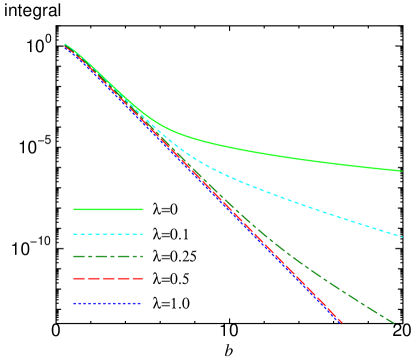
Figure 1: Impact parameter dependences of (14) for various $\lambda$ are plotted for $r=0.1$ at $\cos\theta=0$. Solid, short dashed, dot-dashed, dashed and dotted lines correspond to those for $\lambda=0,0.1,0.25,0.5$ and $1$.

First consider what happens if we keep $r$ finite and go to large $b$. Unless $\vec{z}\sim\pm 2\vec{b}$, the functions $N$ in the BK equation are exponentially small. If this is satisfied, then the kernel of the equation is of order $e^{-4\lambda b}$ so that we preserve the form of the solution so long as $\lambda\geq\mu/2$ because the distribution in the kernel is factorized in Eq. (9). (We expect that $\mu\geq m_{\pi}$ for the large distance asymptotics of the regulated BFKL kernel, as noted in Sec. 1. Therefore this constraint is a rather weak one.) In order to be precise, we evaluate the following integral corresponding to the right-hand side of the BK equation

$$\int d^{2}z\frac{(x-y)^{2}}{(x-z)^{2}(z-y)^{2}}e^{-\lambda|x-z|}e^{-\lambda|z-y|}$$

$$\hskip 56.9055pt\times\bigl{(}N_{0}(x,z)+N_{0}(z,y)-N_{0}(x,y)-N_{0}(x,z)N_{0}(z,y)\bigr{)}\,,$$ (14)

with the initial condition (8) together with (11). Throughout this paper, we use the unit $\mu\equiv 1$ and set $c=8.0$ in (11) in numerical calculations. Figure 1 shows the impact parameter dependence of this integral for dipole size $r=0.1$ and orientation $\cos\theta\equiv\vec{r}\cdot\vec{b}/rb=0$. Here, we have assumed cylindrical symmetry and dropped the dependence on the azimuthal angle. This clearly shows that, while the power law tail is generated for $\lambda=0$, the exponential falling tail in the initial condition can be maintained for $\lambda\geq\mu/2$. This power law tail can be seen in Fig. 7 of [15] where the same integral with no infrared cutoff has been evaluated for the initial condition of the Glauber-Muller form with a steeply falling profile in $b$, that is, $e^{-b^{2}}$. Therefore, the massless property of the BK kernel, not the form of the (initial) distribution, may originate the power law tail in impact parameter. For $\lambda\leq\mu/2$, the behaviour of the integral can be shown to be $e^{-4\lambda b}/b^{4}$, from the structure of the integral, and this fits the observed distribution well.

Now consider what happens if we take the limit that $r\rightarrow\infty$ with $b\gg 1/\mu$, but $b$ fixed. In this case, the kernel vanishes, and the distribution function maintains its original form, as seen in numerical solutions below. This is good because in this region there is little matter, but one is in the non-perturbative region. On general grounds, the distribution function should tend to one in this region, and should not be much affected by evolution due to the presence of the Color Glass Condensate.

Note also that if we look at the problem term which generated long distance singular behaviour in our original analysis of the massless unregulated kernel, we need to look at $r\sim R$ and $b\sim R/2$. The potentially dangerous region comes from $z\sim-R/2$. Then this contribution is suppressed by $e^{-\lambda R}$ from the regulated kernel which is small so long as $\lambda\geq\mu/2$ as was the case above.

To summarize, the modification of the kernel we propose does in fact have the correct properties to preserve the behavior we expect of $N_{Y}(r,b)$ based on general principles.

3 An Equation Ignoring Impact Parameter Diffusion

3.1 Discussion

The Balitsky-Kovchegov equation as written in the $r,b$ basis as in Eq. (13) generates a power law tail in inverse impact parameter if the kernel is not regulated. On the other hand, the regulated kernel generates no such tail. This suggests that if we compute the distribution function $N(r,b)$ on scales of $r$ which are small compared to the scale of variation in $b$, then one may be able to ignore impact parameter diffusion.

Looking at Eq. (13), we see that if the exponential tail of the impact parameter cutoff satisfies $\lambda\geq\mu/2$, then the dominant contribution in the integration over z comes from $z\sim r$. In the region where $z\sim 1/\mu$, we get a contribution of order $r^{2}\mu^{2}$. Clearly, ignoring impact parameter diffusion should be valid so long as we have a cutoff kernel.

In practical terms, this means that a good lowest order approximation should be generated if we expand the terms inside Eq. (13)

$$N(r^{\prime},b^{\prime})=N(r^{\prime},b+\Delta b)$$ (15)

in powers of $\Delta b$, and keep the first non-leading terms. The lowest order term in this gives an equation local in impact parameter (after transforming $z\to z-\frac{1}{2}r$)[12]

$${\partial\over{\partial Y}}N_{Y}(r,b) = \overline{\alpha}\int{d^{2}z}{r^{2}\over{\mid r-z\mid^{2}\mid z\mid^{2}}}e^{-\lambda\mid r-z\mid}e^{-\lambda\mid z\mid}\bigl{(}N_{Y}(r-z,b)$$ (16)

$$\hskip 28.45274pt+N_{Y}(z,b)-N_{Y}(r,b)-N_{Y}(r-z,b)N_{Y}(z,b)\bigr{)}\,.$$

This equation clearly preserves the initial conditions at large impact parameter. If $r\ll 1/\mu$, it also has the property that one can ignore the $\lambda$ dependence in the evolution equation, so long as $\lambda\geq\mu/2$, as we shall assume. This means the solution to this equation has all the properties assumed in Ref. [11], where the Froissart bound was argued to be true when measurements were made at scales $Q^{2}\gg\mu^{2}$.

The solution to this equation should be roughly of the following form: In the limit where the distribution function is itself small and where $r\ll 1/\lambda$, the solution is the ordinary $BFKL$ solution of the linear $BFKL$ evolution equation times an impact parameter profile. This solution will hold until the function $N$ becomes of order 1. This should occur roughly when

$$(rQ_{sat}(Y))^{\gamma}e^{-\mu b}\sim 1\,,$$ (17)

or

$$r\sim\frac{e^{\mu b/\gamma}}{Q_{sat}(Y)}$$ (18)

where $Q_{sat}(Y)$ is the saturation momentum of the ordinary BK equation. For rapidities beyond the critical rapidity for which the amplitude $N_{Y}(r,b)$ first becomes of order 1, the amplitude remains of order 1 for larger rapidity because the BK equation doesn’t violate the unitarity.

On the other hand, when $r\geq 1/\lambda$, the kernel of the BK equation introduced above cuts off further evolution, and the function $N_{Y}(r,b)$ is frozen to its initial condition.

It is difficult to get a direct computation of the correction to the zero impact parameter diffusion approximation. Naive expansion in a Taylors series around zero impact parameter diffusion leads to an equation with mild infrared singularities. Nevertheless, the estimate made above, that these corrections should be of order $r^{2}\mu^{2}$, up to logarithms, is still true. This of course requires that $\lambda\geq\mu/2$. If this was not true, the tail of the distribution would be modified in an unmanageable way. Nevertheless, the leading order solution is valid so long as we study small $r$, and does not requires that $\lambda\geq\mu/2$. On the other hand, at large $r$, our form of the kernel has the physically plausible behavior that $N_{Y}(r,b)$ does not evolve in $Y$.

3.2 Numerical Solutions

In this section, numerical solutions of Eq. (16) for $\lambda=0$ and $1$ are calculated. We used the same parameters $\alpha_{S}=0.2$, $N_{c}=3$ and $c=8$ in the initial condition (8) together with (11), as in Sec. 2. Since Eq. (16) is local in $b$ and our initial condition depends only on $r(\equiv|\vec{r}|)$ and $b(\equiv|\vec{b}|)$ but not on the angle $\theta$ between $\vec{r}$ and $\vec{b}$, the solution $N_{Y}$ at any rapidity has the same property, that is, $N_{Y}(\vec{r},\vec{b})=N_{Y}(r,b)$.

The numerical method to solve Eq. (16) is similar to the one for the solutions of the full BK equation [15], and highest rapidity in our calculations is 40.

3.2.1 The dipole size dependence of the solution

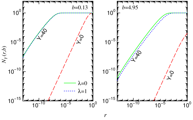
Figure 2: The $r$ dependence of distribution functions for $b=0.13$ (left panel) and $4.95$ (right panel). Dashed lines represent the initial distribution. Solid and dotted lines correspond to the distributions for $\lambda=0$ and $1$ at $Y=40$.

First, let us examine the rapidity evolution of the distribution function for small dipole sizes $r<1$. In Fig. 2, the distribution functions for $\lambda=0$ and $1$ are plotted as a function of $r$. Left and right panels correspond to the distributions at $b=0.13$ and $4.95$. In each panel, the dashed line is the initial distribution, and solid and dotted lines are the distributions for $\lambda=0$ and $1$ at highest rapidity $Y=40$. While the distribution functions for $\lambda=0$ and $1$ are in good agreement for small $b(=0.13)$ as shown in the left panel, the evolution for $\lambda=1$ is slightly suppressed for large $b(=4.95)$ in the right panel. We also found the exponent for small $r$ changes from $r^{2}$ in the initial distribution to $r^{2\gamma_{0}}$ with $\gamma_{0}\sim 0.6-0.7$ at high rapidities, independently of $b$ and $\lambda$ [13]-[14]. This $\gamma_{0}$ is called anomalous dimension and the value is consistent with other studies [11].

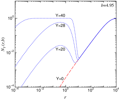
Figure 3: The distribution function at $b=4.95$ for $\lambda=1$ is plotted as a function of $r$ at various rapidities.

Next, let us examine how the regulated kernel affects the evolution of large dipole size. Figure 3 shows the distribution function at $b=4.95$ for $\lambda=1$ including the region $r>1/\lambda$ where the regulated kernel may affect the evolution. It is observed in this figure that the evolution of the distribution function is suppressed around $r\sim 1(=1/\lambda)$ and the distribution is frozen to its initial value in the region $r\gg 1$, as we mentioned in the previous section. If the initial distribution reaches to its saturated value in the region $r\gtrsim 1/\lambda$, it doesn’t evolve any further in such region and the regulated kernel doesn’t affect its evolution. This is the case for small $b$ in our initial condition, as you can see in the left panel of Fig. 2.

That said, the dip shown in Fig. 3 for large $r$ is in an unphysical region where the separation of the sources of color charge within the dipole are at unphysical size scales. This is a region dominated by non-perturbative physics, and ascribing physics to this region is no doubt problematic. This region causes no problem in the solution of the equation we consider, and the dip is presumably an artifact of an incomplete non-perturbative treatment of the correlation function.

3.2.2 The impact parameter dependence of the solution

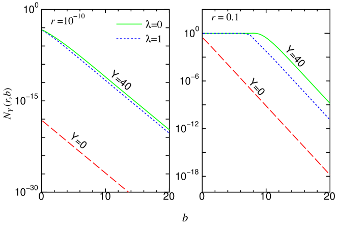
Figure 4: The distribution functions for fixed $r$ at $Y=0$ and $40$ are plotted as a function of $b$. Left and right panels correspond to the distributions for $r=10^{-10}$ and $0.1$. Dashed lines represent the initial distribution. Solid and dotted lines correspond to the distributions for $\lambda=0$ and $1$.

In Fig. 4, the impact parameter dependences of the distributions at fixed $r$ are plotted for $Y=0$ and $40$. It is clearly observed that the exponential falling behavior in the initial condition is maintained at high rapidities both for $\lambda=0$ and $1$, as we expected above. While, for small dipole size $r=10^{-10}$, the distribution functions for $\lambda=0$ and $1$ at high rapidities are in good agreement, the evolution for $\lambda=1$ is a little suppressed compared to that for $\lambda=0$ for $r=0.1$ due to the regulated kernel.

3.2.3 Saturation scale

Next, let us examine the rapidity evolution of the saturation scale $Q_{sat}(Y)$. We define $Q_{sat}(Y,b)$ as an inverse of the lowest $r$ satisfying

$$N_{Y}(r=1/Q_{sat}(Y,b),b)=\kappa\,,$$ (19)

where $\kappa$ is order of unity. The explicit value of $\kappa$ doesn’t matter and $\kappa$ is set to 1/2 below. This definition is the same as in Ref. [15].

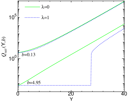
Figure 5: The saturation scale for $\lambda=0$ (solid line) and $1$ (dotted line) are plotted as a function of rapidity. Upper and lower lines correspond to $Q_{sat}(Y,b)$ for $b=0.13$ and $4.95$.

Figure 5 shows the saturation scale for $b=0.13$ and $4.95$ as a function of rapidity. As you can see, the rapidity evolutions with $\lambda=0$ and $1$ almost coincide for small $b$ (=0.13 in this figure), in other words, the infrared cutoff doesn’t change the evolution of the saturation scale for the small impact parameter.

For large $b(=4.95)$, the saturation scale for $\lambda=0$ evolves similarly to that for $b=0.13$. On the other hand, the $Q_{sat}$ for $\lambda=1$ stays in its initial value until the rapidity goes beyond a certain value, and then starts evolving. Looking carefully at Fig. 3, we can understand this behavior. As rapidity increases, the height of the bump of the distribution for $\lambda=1$ around $r\sim 1$ also increases. Until the height of the bump reaches to $\kappa$ in (19), the $Q_{sat}(Y,b)$ is frozen to its initial value. (We should note that nothing particularly exciting is happening with the correlation function itself when $Q_{sat}$ makes a jump, and the jump is no doubt an artifact of its definition, rather than corresponding to some rapid change in a physical quantity.) When the height reaches to $\kappa$ (at $Y\sim 28$ for $b=4.95$), the $Q_{sat}$ jumps to the lowest $r$ satisfying (19) from the initial value $1/Q_{sat}(Y=0)$ and then evolves normally because this is the region $Q_{sat}(Y,b)>\lambda$, e.g., $r<1/\lambda$ and the evolution of the distribution is not affected by the regulated kernel. The point at which the $Q_{sat}(Y,b)$ jumps from the initial value and starts evolving is a monotonically increasing function of $b$. For example, the $Q_{sat}$ at $b=3.3(4.95,7.4)$ has a jump at $Y\sim 20(28,40)$, and for $b>7.4$, the $Q_{sat}$ for $\lambda=1$ is still frozen to its initial value because of the highest rapidity $Y=40$ in our calculations.

It is noted that the slopes at high rapidities are almost same independently of $b$ and $\lambda$, which means the saturation scale at high rapidities can be factorized in the form

$$Q_{sat}(Y,b)\sim exp(2\pi\lambda_{s}\bar{\alpha}Y)\times N(b)\,,$$ (20)

where $N(b)$ is an impact parameter profile function. In our calculation, $\lambda_{s}$ is estimated around $2.1$ which is consistent with that from the full BK equation [15]. This might mean that the rapidity evolution of $Q_{sat}(Y,b)$ is not sensitive to the impact parameter diffusion.

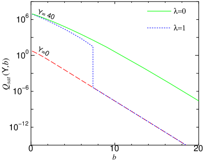
Figure 6: The impact parameter dependence of the saturation scale for $\lambda=0$ (solid line) and $1$ (dotted line) is plotted at $Y=0$ and $40$.

In Fig. 6, the $b$ dependence of the saturation scale for $\lambda=0$ and $1$ is plotted at $Y=0$ and $40$. For small $b$, especially $b<1$, the impact parameter dependences for $\lambda=0$ and $1$ agree well. This is because the evolution of the distribution function for small $b$ doesn’t change by the vacuum property of the regulated kernel, as seen in the left panel of Fig. 2.

We also found the exponential tail of the saturation scale for $\lambda=0$ is maintained at high rapidities, e.g., $e^{-2b}$. Of course, this exponential tail is totally different from that from the full BK equation without infrared cutoff of the kernel, which reads the power-like tail $Q_{sat}(Y,b)\sim 1/b^{\gamma}$ with $\gamma=1.6-2.0$ at high rapidities [15]. The exponential tail is preserved only when the kernel of the BFKL equation is properly regulated in the infrared.

4 The Growth of Black disc radius and The Froissart bound

One of the most important issues in the saturation physics is how fast the black disc radius in which $N_{Y}$ saturates grows in rapidity. This is closely related to the problem of the Froissart bound [9] which tells us that the total hadronic cross section is bounded by

$$\sigma=\frac{2\pi}{m_{\pi}^{2}}\ln^{2}(s/s_{0})\,,$$ (21)

with energy $s\sim e^{Y}$. We define the black disc radius $R_{BD}(r,Y)$ as

$$N_{Y}(r,b=R_{BD}(r,Y))=\kappa\,,$$ (22)

where $\kappa$ is order of unity and $\kappa=1/2$ is chosen as in the case of the saturation scale.

In the saturation regime, the total dipole-nucleus cross section is given by integrating the scattering probability $N_{Y}$ over the impact parameter,

$$\sigma(r,Y)=2\int d^{2}bN_{Y}(r,b)\sim 2\pi R_{BD}^{2}(r,Y)\,.$$ (23)

If this $R_{BD}$ grows at most linearly with the rapidity $Y$, the Froissart bound is saturated. Let us discuss this below.

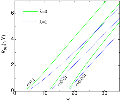
Figure 7: The black disc radius for $\lambda=0$ (solid lines) and $1$ (dotted lines) is plotted as a function of rapidity at $r=0.1,0.01$ and $0.001$ from the left to right.

Figure 7 shows the rapidity dependence of the black disc radius for various dipole sizes. As we can see, in both cases for $\lambda=1$ and $0$, $R_{BD}$ grows linearly as a function of rapidity. The slope at high rapidities for $\lambda=0$ is slightly larger than that for $\lambda=1$ which doesn’t depend on the dipole size if it is small enough ($r<1$). One might think it’s a natural consequence of the local approximation ignoring the impact parameter diffusion. The important point, however, is that this linear growth of the black disc radius in $Y$ is expected in the full BK evolution equation if the kernel of the equation is regulated by the infrared cutoff, although the naive BK equation shows the exponential growth and violates the Froissart bound.

5 Summary

The origin of the infrared cutoff in our analysis needs some understanding beyond what we present here. It is clear that the lower bound we have is a weak one and that the generic feature of Froissart bound saturation appears to be insensitive to details of this cutoff. It is however not clear to us what sets the scale of this cutoff. Is it $2m_{\pi}$, or $2m_{\rho}$? Might one derive an effective meson theory which can generate a BFKL like equation to describe this non-perturbative region? Of course, it is purely non-perturbative and cannot be explained by the perturbative QCD.

Although the considerations presented here are far from rigorous, it seems that one does in fact have a simple intuitive picture of how the Froissart bound arises. It is simply the trade off between the exponential growth of the gluons as a function of rapidity filling up and exponentially falling tail of an impact parameter distribution set by initial conditions.

6 Acknowledgements

L.M gratefully acknowledges conversations with Edmond Iancu and J. Bartels on the subject of this talk. T.I is much grateful to S. Munier and A. M. Stasto for numerous valuable discussions. T.I was supported through a Special Postdoctoral Researcher Program of RIKEN. This manuscript has been authorized under Contract No. DE-AC02-98H10886 with the U. S. Department of Energy.

References

-
[1]
L. N. Lipatov,
Sov. J. Nucl. Phys. 23 (1976) 338;
E. A. Kuraev, L. N. Lipatov and V.S. Fadin, Sov. Phys. JETP 45 (1977) 199;
I. I. Balitsky and L. N. Lipatov, Sov. J. Nucl. Phys. 28 (1978) 822. - [2] I. Balitsky, Nucl. Phys. B 463 (1996) 99.
-
[3]
Yu. V. Kovchegov,
Phys. Rev. D 60 (1999) 034008;
Yu. V. Kovchegov, Phys. Rev. D 61 (2000) 074018. -
[4]
L. Gribov, E. Levin and M. Ryskin,
Phys. Rept. 100 (1983) 1;
A. H. Mueller and Jian-wei Qiu, Nucl. Phys. B 268 (1986) 427;
J.-P. Blaizot and A. H.D Mueller, Nucl. Phys. B 289 (1987) 847. -
[5]
L. D. McLerran and R. Venugopalan,
Phys. Rev. D 49 (1994) 2233;
L. D. McLerran and R. Venugopalan, Phys. Rev. D 49 (1994) 3352;
L. D. McLerran and R. Venugopalan, Phys. Rev. D 50 (1994) 2225. -
[6]
E. Iancu, A. Leonidov and L. D. McLerran,
Nucl. Phys A 692 (2001) 583;
E. Ferreiro, E. Iancu, A. Leonidov and L. D. McLerran, Nucl. Phys. A 710 (2002) 373;
E. Iancu and L. McLerran, Phys. Lett. B 510 (2001) 145. -
[7]
J. Jalilian-Marian, A. Kovner, L. McLerran and H. Weigert,
Phys. Rev. D 55 (1997) 5414;
J. Jalilian-Marian, A. Kovner, A. Leonidov and H. Weigert, Nucl. Phys. B 504 (1997) 415;
J. Jalilian-Marian, A. Kovner, A. Leonidov and H. Weigert, Phys. Rev. D 59 (1999) 014014. -
[8]
E. Gotsman, M. Kozlov, E. Levin, U. Maor and E. Naftali,
Nucl. Phys. A 742 (2004) 55;
A. Kovner and U. A. Wiedemann, Phys. Rev. D 66 (2002) 034031;
K. Golec-Biernat, L. Motyka and A. Stasto, Phys. Rev. D65 (2002) 074037;
M. Braun, Eur. Phys. J. C16 (2000) 337;
N. Armesto and M. Braun, Eur. Phys. J. C20 (517 (2001). -
[9]
M. Froissart,
Phys. Rev. 123 (1961) 1053;
A. Martin, Phys. Rev. 129 (1963) 1432. - [10] A. Kovner and U. A. Wiedemann, Phys. Lett. B 551 (2003) 331.
- [11] E. Ferreiro, E. Iancu, K. Itakura, and L. McLerran, Nucl. Phys. A 710 (2002) 373.
- [12] S. Bondarenko, M. Kozlov and E. Levin, Nucl. Phys. A 727 (2003) 139.
- [13] E. Iancu, K. Itakura and L. McLerran, Nucl. Phys. A 708 (2002) 327.
-
[14]
A. H. Mueller and V. N. Triantafyllopoulos,
Nucl. Phys. B 640 (2002) 331;
D. N. Triantafyllopoulos, Nucl. Phys. B 648 (2003) 293. - [15] K. Golec-Biernat and A. M. Stasto, Nucl. Phys. B 668 (2003) 345.